CopyrightÓ2010 by the Genetics Society of America DOI: 10.1534/genetics.110.114280
Genomewide Multiple-Loci Mapping in Experimental Crosses by Iterative
Adaptive Penalized Regression
Wei Sun,*
,†,1Joseph G. Ibrahim* and Fei Zou*
*Department of Biostatistics and†Department of Genetics, University of North Carolina, Chapel Hill, North Carolina 27599
Manuscript received January 17, 2010 Accepted for publication February 3, 2010
ABSTRACT
Genomewide multiple-loci mapping can be viewed as a challenging variable selection problem where the major objective is to select genetic markers related to a trait of interest. It is challenging because the number of genetic markers is large (often much larger than the sample size) and there is often strong linkage or linkage disequilibrium between markers. In this article, we developed two methods for genomewide multiple loci mapping: the Bayesian adaptive Lasso and the iterative adaptive Lasso. Compared with eight existing methods, the proposed methods have improved variable selection performance in both simulation and real data studies. The advantages of our methods come from the assignment of adaptive weights to different genetic makers and the iterative updating of these adaptive weights. The iterative adaptive Lasso is also computationally much more efficient than the commonly used marginal regression and stepwise regression methods. Although our methods are motivated by multiple-loci mapping, they are general enough to be applied to other variable selection problems.
I
T is well known that complex traits, including many common diseases, are controlled by multiple loci (Hohand Ott2003). However, multiple-loci mapping remains one of the most attracting and most difficult problems in genetic studies, mainly due to the high dimensionality of the genetic markers as well as the com-plicated correlation structure among genotype profiles (throughout this article, we use the term ‘‘genotype profile’’ to denote the genotype profile of one marker, instead of the genotype profile of one individual). Suppose a quantitative trait and the genotype profiles of p0 markers (e.g., single-nucleotide polymorphisms, SNPs) are measured in n individuals. We treat this multiple-loci mapping problem as a linear regression problem,yi¼b01 Xp
j¼1
xijbj1ei; ð1Þ
ory¼b01Xb1ein a matrix form, wherey¼(y1,. . ., yn)T, X ¼(xij)n
3p, b0¼ b0113p, b ¼(b1, . . ., bp)T, e ¼ (e1,. . .,en)T, andeN(0
n31,s2In3n).yiis the trait value of theith individual, andb0is the intercept. Herepis the total number of covariates. If we consider only the main effect of each SNP,p¼p0; and if we consider the main effects and all the pairwise interactions,p¼p01p0(p0–
1)/2.xijis the value of thejth covariate of individuali. The specific coding ofxijdepends on the study design and the inheritance model. For example, if additive inheritance is assumed, the main effect of a SNP can be coded as 0, 1, and 2 on the basis of the number of minor alleles. The major objective of multiple-loci mapping is to identify the correct subset model, i.e., to identify thosej’s, such thatbj6¼0, and estimate thebj’s.
Marginal regression and stepwise regression are com-monly used for multiple-loci mapping. Permutation-based thresholds for model selection have been used for these two methods (Churchilland Doerge1994; Doerge and Churchill 1996). Broman and Speed (2002) proposed a modified Bayesian information criterion (BIC) for model selection, which was further written as a penalized LOD score criterion and imple-mented within a forward–backward model selection framework (Manichaikulet al.2009). The threshold of the penalized LOD score is also estimated by permutations.
Several simultaneous multiple-loci mapping methods have been developed, among which two commonly used approaches are Bayesian shrinkage estimation and Bayesian model selection. Most existing Bayesian shrinkage methods are hierarchical models based on the additive linear model specified in Equation (1), with covariate-specific priors: p(bjjs2j) N(0, s
2 j). The coefficients are shrunk because their prior mean values are 0. The degree of shrinkage is controlled by the prior of the covariate-specific variances2
j. An inverse-Gamma prior,
Supporting information is available online athttp://www.genetics.org/ cgi/content/full/genetics.110.114280/DC1.
1Corresponding author:University of North Carolina, 4105E McGavran Greenberg Hall, Chapel Hill, NC 27599. E-mail: [email protected]
pðs2
jjd;tÞ ¼inv-Gammaðd;tÞ ¼ t
d
GðdÞ
s2j1dexpt s2
j
; ð2Þ
leads to an unconditional prior of bj as a Student’s t distribution (Yiand Xu2008). We refer to this method as the Bayesian t. Another choice is an exponential prior,
ps2jja 2 2
¼Expa 2 2
¼a 2 2exp
a
2 2 s
2 j
; ð3Þ
where a is a hyperparameter. In this case, the un-conditional prior ofbjis a Laplace distribution,pðbjÞ ¼ ða=2Þeajbjj that is closely related to the Bayesian
interpretation of the Lasso (Tibshirani1996); there-fore, it has been referred to as the Bayesian Lasso (Yi and Xu 2008). Park and Casella (2008) con-structed the Bayesian Lasso using a similar but distinct prior: p(bjjs2j) N(0, s
2 es
2
j) and p(s 2 j ja
2/2) ¼ Exp(a2/2). Hans(2009) proposed another Bayesian Lasso method, with more emphasis on prediction than on variable selection. Several general Bayesian model selection methods have been applied for multiple-loci mapping, for example, the stochastic search variable selection (George and McCulloch 1993) and the reversible-jump Markov chain Monte Carlo (MCMC) methods (Richardson and Green 1997). One example is the composite model space approach (CMSA) (Yi2004).
We propose two variable selection methods: the Bayesian adaptive Lasso (BAL) and the iterative adap-tive Lasso (IAL). The BAL is a fully Bayesian approach while the IAL is an expectation conditional maximiza-tion (ECM) algorithm (Mengand Rubin1993). Both the BAL and the IAL are related to the adaptive Lasso (Zou 2006), which extends the Lasso (Tibshirani 1996) by allowing covariate-specific penalties. The adaptive Lasso enjoys the oracle property (Fan and Li2001);i.e., the covariates with nonzero coefficients will be selected with probability tending to 1, and the estimates of nonzero coefficients have the same as-ymptotic distribution as the correct model. However, the adaptive Lasso requires consistent initial estimates of the regression coefficients, which are generally not available in the high dimension, low sample size (HDLSS) setting. Huang et al. (2008) showed that with initial estimates obtained from the marginal regression, the adaptive Lasso still has the oracle property in the HDLSS setting under a partial orthog-onality condition: the covariates with zero coefficients are weakly correlated with the covariates with nonzero coefficients. However, in many real-world problems, including the multiple-loci mapping problem, the covariates with zero coefficients are often strongly
correlated with some covariates with nonzero coeffi-cients. The BAL and the IAL extend the adaptive Lasso in the sense that they do not require any informative initial estimates of the regression coeffi-cients so that they can be applied in the HDLSS setting, even if there is high correlation among the covariates.
After we completed an earlier version of this article, we noticed an independent work on extending the adaptive Lasso from a Bayesian point of view (Griffin and Brown 2007). There are several differences be-tween Griffin and Brown’s approach and our work. First, Griffin and Brown (2007) did not study the fully Bayesian approach, while we have implemented and carefully studied the BAL. Second, Hoggart et al. (2008) implemented Griffin and Brown’s approach in HyperLasso, a coordinate descent algorithm, which is different from the IAL at both model setup and implementation. We showed in our simulation and real data analysis that the IAL has significantly better vari-able selection performance than the HyperLasso. The differences between the IAL and the HyperLasso are further elaborated in thediscussion.
In this article, we focus on the genomewide multiple-loci mapping in experimental crosses of inbred strains (e.g., yeast segregants, F2 mice) where typically thou-sands of genetic markers are genotyped in hundreds of samples. Another situation is genomewide associa-tion studies (GWAS) in outbred populaassocia-tions where millions of markers are genotyped in thousands of indi-viduals. Multiple-loci mapping in experimental crosses and GWAS presents different challenges. In experimen-tal crosses, genotype profiles have higher correlations in longer genomic regions, which give simultaneous multiple-loci mapping methods more advantages than the marginal regression or stepwise regression. In contrast, GWAS data have higher dimensionality but the linkage disequilibrium (LD) blocks often have limited sizes. We focus on the experimental cross in this study, but similar methods can also be applied to GWAS data, although preselection or mapping chromosome-by-chromosome may be necessary to reduce the di-mension of the covariates.
The remainder of this article is organized as follows. We first introduce the BAL and the IAL in the following two sections, respectively, and then evaluate them and several existing methods by extensive simulations in simulation studies. A real data study of multiple-loci mapping of gene expression traits is presented in the gene expression QTLstudy section. We summarize and discuss the implications of our methodology in the discussion.
THE BAL
The BAL is a Bayesian hierarchical model. The priors are specified as
pðb0Þ}1; pðs2eÞ} 1
s2e; ð4Þ
pðbjjkjÞ ¼ 1 2kj
exp jbjj kj
; ð5Þ
pðkjjd;tÞ ¼inv-Gammaðkj;d;tÞ ¼
td
GðdÞk 1d
j exp
t kj
; ð6Þ
whered .0 andt.0 are two hyperparameters. The unconditional prior ofbjis
pðbjÞ ¼ ð‘
0 td 2GðdÞk
2d j exp
ð jbjj1tÞ kj
dkj ¼t
dd
2 ð jbjj1tÞ
1d; ð7Þ
which we refer to as apowerdistribution with parameters dandt. From this unconditional prior, we can see that smaller t and larger d lead to bigger penalization. In practice, it could be difficult to choose specific values for the hyperparameters d and t. Following a similar rationale of Yi and Xu (2008), we suggest a joint im-proper priorp(d,t)}t1and let the data estimatedand t. We suggest the prior oft1because in our application in the HDLSS setting, we encourage larger penalty and hence smallertand largerd.
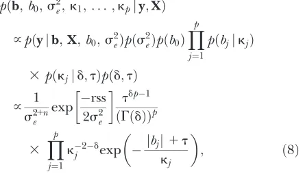
The posterior distribution of all the parameters is given by
pðb;b0; s2e;k1;. . . ;kpjy;XÞ }pðyjb;X;b0;s2eÞpðs2eÞpðb0Þ
Yp j¼1
pðbjjkjÞ 3 pðkjjd;tÞpðd;tÞ
} 1 s21n
e
exp rss 2s2e
tdp1 ðGðdÞÞp
3 Y
p
j¼1 k2d
j exp
jbjj1t kj
; ð8Þ
where rss indicates residual sum of squares, i.e., Pn
i¼1ðyib0Ppj¼1xijbjÞ 2
. We sample from this poste-rior distribution using a Gibbs sampler, which is presented insupporting information,File S1, Section A. Our model can also be explained from the perspec-tive of penalized least squares. Using the unconditional prior to replace the conditional prior, and taking the negative logarithm of the posterior probability, we obtain a penalized least-squares objective function: rss/(2s2
e)1 (11d) log(jbjj1t), with a log penalty forjbjj. Another form of log penalty is l log(jbjj), which has been introduced by Zouand Li(2008) as the limit of bridge penaltyjbjjg
, asg/0. Comparing these two forms of log penalties,land 11d are both tuning parameters that
control the size of the penalty, and our log penalty has an extra parametertto give a minimum penalty whenbj¼0. In contrast, ifbj¼0, the log penalty by Zouand Li(2008) is infinite, which is not a problem for their one-step estimate, given the initial estimate ofbjis not zero, but will cause problems in our iterative algorithms. Friedman (2008) proposed a log penalty,llog((1 –b)jbjj1b), with 0,b,1, which is equivalent to the log penalty that we use. Friedman’s motivation is that this log penalty bridges the L1 penalty (Lasso) and the L0 penalty (all-subset selection) as b changes from 1 to 0. In contrast, we motivate this log penalty and solve the penalized least-squares problem from a Bayesian point of view.
The BAL can be better understood by comparing it with the Bayesian Lasso. Recall that in the Bayesian Lasso, bjjs2j N(0, s
2 j), s
2
j Exp(a
2/2), and the unconditional prior for eachbjis a double-exponential distribution. The conditional normal prior resembles a ridge penalty and the unconditional Laplace prior resembles a Lasso penalty. Therefore an intuitive (albeit not accurate) explanation of the Gibbs sampler for the Bayesian Lasso is that it approaches a Lasso penalty by iteratively applying covariate-specific ridge penalties. Figure 1 in Parkand Casella(2008) justifies this intui-tive explanation: the coefficient paths of the Bayesian Lasso are a compromise between the coefficient paths of the Lasso and ridge regression. In contrast, an intuitive explanation of the BAL is that it approaches the log penalty by iteratively applying the adaptive Lasso penalty. Figure 1 illustrates the difference between the uncondi-tional prior distribution of BAL and the Bayesian Lasso. The former has a higher peak at zero and heavier tails, which leads to more penalization for smaller coefficients and less penalization for larger coefficients. This shape can potentially be an advantage in the HDLSS setting
Figure 1.—Comparison of the power distribution
fðx;t;dÞ ¼ ðtdd=2Þðjxj1tÞ1d
, given t ¼ 0.02 and d ¼ 0.1, and the Laplace (i.e., double exponential, DE) distribu-tionfðx;kÞ ¼ ð1=2kÞexpðjxj=kÞ, givenk¼1 or 0.2. We plot the density in log scale for better illustration. The power dis-tribution tends to have a higher peak at zero and heavier tails for larger values.
where strong penalty is needed, although as pointed by a reviewer, what shape works best depends on the data.
THE IAL
Because no point mass at zero is specified in the Bayesian shrinkage methods (including the BAL), the samples of the regression coefficients would not be exactly zero, and thus the Bayesian shrinkage methods do not automatically select variables. However, if we look for the mode of the posterior distribution, it could be exactly zero. This leads to the following ECM algorithm: the iterative adaptive Lasso. Specifically, under the setup of the BAL (Equations 4–6), we treatu¼(b0,b1,. . .,bp) as parameter and letf¼(s2
e,k1,. . .,kp) be the missing data. The observed data areyiandxij. The complete data log-posterior ofuis
lðujy;X;fÞ ¼C rss 2s2e
Xp j¼1
jbjj
kj ; ð9Þ whereCis a constant with respect tou. Suppose in thetth iteration the parameter estimates are u(t) ¼ ðbð0tÞ;b
ðtÞ 1 ;. . .;b
ðtÞ
p Þ. Then after some derivations (File
S1, Section B), the conditional expectation ofl(ujy,X,f) with respect to the conditional density off(fjy,X,u(t)) is
QðujuðtÞÞ ¼
C rss=2 rssðtÞ=n
Xp j¼1
jbjj ð jbðjtÞj1tÞ=ð11dÞ
; ð10Þ
where rss(t) is the residual sum of squares calculated on the basis of u(t) ¼ ðbðtÞ
0 ;b ðtÞ 1 ;. . .;b
ðtÞ
p Þ. Com-paring Equations 9 and 10, it is obvious that to obtain Q(uju(t)), we can simply lets2
e¼rss
(t)/nandk j¼(jb
ðtÞ j j1 t)/(11d).
On the basis of the above discussions, the IAL is implemented as follows:
1. Initialization: We initializebj(0 # j# p) with zero, initializes2
e by variance ofy, and initializekj(1#j# p) witht/(11d).
2. Conditional maximization (CM) step:
a. Update b0 by its posterior mode (see File S1, Section B for more details), b0¼ ð1=nÞPni¼1 yiPpj¼1xijbj
.
b. Forj¼1,. . .,p, updatebjby its posterior mode (seeFile S1, Section B),
bj¼0 if
s2 j kj #
bj# s2
j kj bj¼bj
s2 j kj if
bj. s2
j kj bj ¼bj1
s2 j kj if
bj, s2
j kj ; 8 > > > > < > > > > : where s2 j ¼
s2e Pn
i¼1xij2 ;
and
bj¼ Xn
i¼1
xij2 !1
Xn i¼1
xij yib0 X
k6¼j xikbk 0
@
1 A:
3. Expectation (E) step: With the updatedbj’s, recalcu-late the residual sum of squares, rss, and do the following:
a. Updatese2:se2¼rss/n.
b. Updatekj:kj¼(jbjj1t)/(11d).
We say the algorithm is converged if the coefficient estimatesˆb0;ˆb1;. . . ;ˆbp have little change.
The above discussions proved that the IAL is an ECM algorithm, which guarantees its convergence. In each step of the ECM algorithm, the conditional log poste-rior is concave, so a local maximum is a global maxi-mum, and thus it is computationally easy to maximize the conditional log posterior. However, the uncondi-tional log prior is not concave; thus for some tuning parameters, the unconditional log posterior (that is, the concave log likelihood plus the nonconcave log prior) could be nonconcave, so that a local maximum many not be the global maximum. Therefore, similar to other EM algorithms, it is possible that the IAL identifies a local mode of the posterior. This is a common problem for EM algorithms and we address this issue by choosing appropriate initial values of the coefficients and appro-priate tuning of the hyperparameterstandd.
In the HDLSS setting, especially where the covariates are highly correlated, initial estimates from ordinary least squares (OLS) or ridge regression are unavailable, unstable, or noninformative. Therefore we initialize all the coefficients by zero.
To decidedandt, we first consider this problem in an asymptotic point of view to show that theoretically, we can identify optimaldandt(see Theorem 1 inFile S1, Section C). However, the theoretical results provide only a rough scale fordandt. In practice, we select the specific values of d and t by the BIC, followed by a variable filtering step. The BIC is written as
BICt;d¼logrss
n 1
logðnÞ
n d:f:t;d; ð11Þ where d.f.t,dis the number of nonzero coefficients, an
estimate of the degrees of freedom (Zou et al. 2007). Given the subset model selected by the BIC, the variable filtering step can be implemented by a single multiple-regression or stepwise backward selection. Multiple regression is computationally more efficient. However, occasionally, if two highly correlated covariates are both included in the model, it is possible that both of them are insignificant by multiple regression. In backward regression, however, after dropping one of them, the other one may become significant. We use backward regression for all the numerical results in this article. TheP-value cutoff for variable filtering can be set as 0.05/ pE, wherepEis the effective number of independent tests.
A conservative choice is pE ¼ p, the total number of covariates. In this article, we estimatepEby the number of independent tests; see Sunand Wright(2010) and
File S1, Section D for details. Our approach is closely related to the screening and cleaning method proposed by Wasserman and Roeder (2009). Wasserman and Roeder(2009) use Lasso, marginal regression, or forward stepwise regression accompanied with cross-validation for screening and use a multiple regression for cleaning. We use the IAL for screening and use multiple regres-sion or backward regresregres-sion for cleaning. As pointed out by an anonymous reviewer, a ridge regression using all the selected covariates may also be an appropriate choice for cleaning.
In contrast to the BIC plus variable filtering approach, an alternative strategy is to apply an extended BIC, which provides larger penalty for bigger models (Chen and Chen 2008). The simulation results in the next section show that the extended BIC leads to slightly worse variable selection performance. Our explanation is that the extended BIC is valid asymptotically and it is conservative when the sample size is relatively small (n¼ 360 in our simulation). Compared with the extended BIC, the ordinary BIC tends to select larger models with all or most of the true discoveries plus some false dis-coveries (Chenand Chen2008), which can be filtered out by the variable filtering step.
SIMULATION STUDIES
We first use simulations to evaluate the variable selec-tion performance of 10 methods: marginal regression, forward regression, forward–backward regression (with penalized LOD as the model selection criterion), the CMSA, the adaptive Lasso (with initial regression co-efficients from marginal regression), the IAL, the HyperLasso, and three Bayesian shrinkage methods: the Bayesiant, the Bayesian Lasso, and the BAL. SeeFile S1, Section E for the implementation details.
Simulation setup: We first simulate a marker map of 2000 markers from 20 chromosomes of length 90 cM, with 100 markers per chromosome [using function sim.map in R/qtl (Bromanet al.2003)]. The chromo-some length is chosen to be close to the average chromosome length in the mouse genome. Next we simulate genotype data of the 360 F2mice on the basis of the simulated marker map (using function sim.cross in R/qtl). As expected, the markers from different chro-mosomes have little correlation, while the majority of the markers within the same chromosome are positively correlated (Figure S1). In fact, given the genetic dis-tance of two SNPs, the expectedR2between two SNPs in this F2cross can be explicitly calculated (Figure S2). For example, theR2’s of two SNPs 1, 5, and 10 cM apart are 0.96, 0.82, and 0.67, respectively. Finally, we randomly choose 10 markers as QTL and simulate quantitative traits in six situations with 1000 simulations per
situa-tion. Given the 10 QTL, the trait is simulated on the basis of the linear model in Equation 1, where genotype (xij) is coded by the number of minor alleles. The QTL effect sizes across the six situations are listed below: 1. Unlinked QTL: One QTL per chromosome, with
effect sizes 0.5, 0.4,0.4, 0.3, 0.3,0.3, 0.2, 0.2,0.2, and0.2;s2
e¼1. Recall thats 2
e is the variance of the residual error.
2. QTL linked in coupling: Two QTL per chromosome, with effect sizes of the QTL for each chromosome as (0.5, 0.3), (0.4, 0.4), (0.3, 0.3), (0.2, 0.2), and (0.2,0.2);s2
e ¼1.
3. QTL linked in repulsion: Two QTL per chromosome, with effect sizes of the QTL for each chromosome as (0.5,0.3), (0.4,0.4), (0.3,0.3), (0.2,0.2), and (0.2,0.2);s2
e ¼1.
Situations 2, 4, and 6 are the same as situations 1, 3, and 5, respectively, except thats2
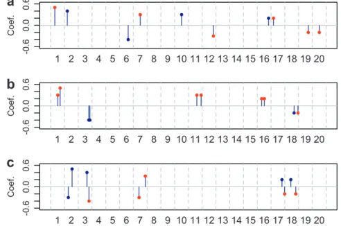
e ¼0.5. The locations and effect sizes of the QTL in each situation are illustrated in Figure 2. To mimic the reality that the genotype of a QTL may not be observed, we randomly select 1200 markers with ‘‘observed genotype profiles’’ and use only these 1200 markers in the multiple-loci mapping. The information loss is limited due to the high density of the markers. In fact, the vast majority of the 800 markers with missing genotype can be tagged withR2. 0.8 by at least one marker with observed genotype (Figure S3).
Figure2.—The locations and effect sizes of the QTL in the simulation study. The markers labeled with red are among the 800 markers with ‘‘missing data’’. (a) Situations 1 and 2. (b) Situations 3 and 4. The genetic distances/R2 between two
QTL from chromosomes 1, 3, 11, 16, and 18 are 15 cM/ 0.63, 7 cM/0.68, 28 cM/0.25, 17 cM/0.56, and 26 cM/0.40, respectively, whereR2denotes the correlation square. (c)
Sit-uations 5 and 6. The genetic distances/R2between two QTL
from chromosomes 2, 3, 7, 17, and 18 are 25 cM/0.31, 13 cM/ 0.59, 41 cM/0.22, 17 cM/0.55, and 33 cM/0.30, respectively. The means (standard deviations) of the proportion of trait variance explained by the 10 QTL in the six simulation situa-tions are 0.31 (0.02), 0.48 (0.03), 0.44 (0.03), 0.62 (0.04), 0.17 (0.01), and 0.29 (0.02), respectively.
One important aspect in the implementation of Bayesian methods is the diagnosis of the convergence of the MCMC. The results inFigure S4,Figure S5, and
Figure S6 suggest the convergence of the Bayesian Lasso, Bayesiant, and BAL, respectively.
Results: We divide the methods to be tested into two groups: the Bayesian methods that do not explicitly carry out variable selection (since most coefficients remain nonzero) and the stepwise regression, adaptive Lasso, and HyperLasso that explicitly select a subgroup of variables. The IAL is classified into the first group if we use the ordinary BIC to select the hyperparameters; and it is classified into the second group if we use the extended BIC or ordinary BIC plus variable filtering.
For either group, we compare the performance of different methods by comparing the number of true discoveries and false discoveries across different cutoffs of coefficient size or posterior probability. Given a cutoff, we can obtain a final model. We count the
number of true discoveries in the final model as follows. For each of the true QTL, we check whether any marker in the final model satisfies the following three criteria: (1) it is located on the same chromosome as the QTL, (2) it has the same effect direction (sign of the co-efficient) as the QTL, and (3) the R2 between this marker and the QTL is.0.8. Different cutoffs such as 0.7 and 0.9 lead to similar conclusions (results not shown). If there is no such marker, there is no true discovery for this QTL. If there is at least one such marker, the one with the highestR2with the QTL is recorded as a true discovery and is excluded from the true discovery searching of other QTL. After the true discoveries of all the QTL are identified, the remaining markers in the final model are defined as false discoveries. These false discoveries are further divided into two classes: false discoveries linked to at least one QTL (linked false discoveries) and false discoveries unlinked to any QTL (unlinked false discoveries). A false discovery is linked to a
Figure3.—Comparison of the number of true discoveriesvs. the total number of false discover-ies in the simulation study.
QTL if it satisfies the above three criteria. We summarize the results of each method by an receiver operating characteristic (ROC)-like curve that plots the median number of true discoveriesvs.the median number of false discoveries across different cutoff values. The methods with ROC-like curves closer to the upper-left corner of the plot have better variable selection performance because they have less false discoveries and more true discoveries. It is possible that a few cutoff values correspond to the same median of false discoveries but different medians of true discoveries. In this case, the largest median of true discoveries is plotted to simplify the figure. In other words, these ROC-like curves illustrate the best possible performance of these methods. Forward regression out-performs marginal regression in all situations. Therefore we omit the results for marginal regression for readability of the figures.
We first compare the Bayesian methods and the IAL (with ordinary BIC). If the linked false discoveries are counted as false discoveries, the IAL has apparent advantages in all situations. Approximately, the perfor-mance of these methods can be ranked as IAL$CMSA$ BAL$ Bayesiant $ Bayesian Lasso (Figure 3). If the linked false discoveries are counted as true discoveries, the performances of different methods are not well separated (Figure S7). Overall the IAL, the BAL, and the CMSA have similar and superior performance, and the Bayesian Lasso has inferior performance. We point out that the comparison of the IAL and the Bayesian methods should be interpreted with caution. The posterior mode estimates of parameters by the IAL provide less information than the fully Bayesian meth-ods. For example, the Bayesian methods provide the distribution of the regression coefficients or the distri-bution of the probability of being included in the model, while the IAL cannot provide such information. Next we compare the stepwise regression method, the HyperLasso, the adaptive Lasso (with initial estimates from marginal regression), and the IAL with extended BIC or ordinary BIC plus variable filtering. These methods tend not to select the unlinked false discover-ies. In fact, the ROC-like curve for each of these methods is exactly the same whether we count unlinked false discoveries as true discoveries or not. If the linked false discoveries are treated as true discoveries, an additional fine-mapping step is needed to pinpoint the location of the QTL in a cluster of linked markers. Therefore, in general, methods that avoid linked false discoveries should be preferred. As shown in Figure 4, the IAL with ordinary BIC plus variable filtering has the best performance while the HyperLasso has the worst performance in all the situations. When the QTL are linked in repulsion, the HyperLasso has no power at all. The adaptive Lasso has similar performance to the IAL when the signal is strong (i.e., QTL linked in coupling); otherwise it has significantly worse performance than the IAL. The stepwise regression and the IAL using the
extended BIC have slightly worse performance than the IAL using ordinary BIC plus variable filtering.
We have compared different methods by ROC-like curves and use somewhat ad hocrules to define true/ false discoveries. In practice, we may need different criteria to define the true/false discoveries. For exam-ple, if there is no missing covariate, we may define the true discovery as the identification of the exact covariate, instead of a highly correlated one. In fact, for prediction, a small number of false discoveries with small coeffi-cients may not affect the prediction accuracy.
GENE EXPRESSION QTL STUDY
QTL study of one particular trait may favor one method by chance. To evaluate our method in real data in a comprehensive manner, we study the gene expression QTL (eQTL) of thousands of genes. The expression of each gene, like other complex traits, is often controlled by multiple QTL (Brem and Kruglyak2005). Therefore multiple-loci mapping has important applications for eQTL studies. In this section, we study eQTL data with .6000 genes and 2956 SNPs in 112 yeast segregants (Bremand Kruglyak2005; Bremet al.2005). The gene
Figure4.—Comparison of the number of true discoveries
vs. the total number of false discoveries in the simulation study.
expression data are downloaded from Gene Expression Omnibus (GEO) (GSE1990). The expression of 6229 genes is measured in the original data. We drop 129 genes that have.10% missing values and impute the missing values in the remaining 6100 genes by R function impute.knn (Troyanskayaet al. 2001). The genotype data were obtained from Rachel Brem. Fifteen SNPs with .10% missing values are excluded from this study, and the missing values in the remaining SNPs are imputed using the function fill.geno in R/qtl (Bromanet al.2003). The neighboring SNPs with the same genotype profiles are combined, resulting in 1027 genotype profiles. With .6000 genes, it is extremely difficult, if not impossible, to examine the QTL mapping results gene by gene to filter out possible linked false discoveries. Therefore, the Bayesian methods that generate lots of linked false discoveries were not applied to these eQTL data.
We apply the IAL, marginal regression, forward re-gression, forward–backward rere-gression, and Hyper-Lasso to these yeast eQTL data to identify multiple eQTL of each gene separately. In other words, we examine the performances of these methods across 6100 traits. The permutationP-value cutoff for marginal regression and stepwise regression is set at 0.05. The parametersdandtof the IAL are selected by ordinary BIC followed by backward regression, with a P-value cutoff 0.05/412, which is based on a conservative estimate of 412 independent tests (seeFile S1, Section D). For the HyperLasso, the ‘‘lambda’’ parameter is set at
ffiffiffi n p
F1ð1
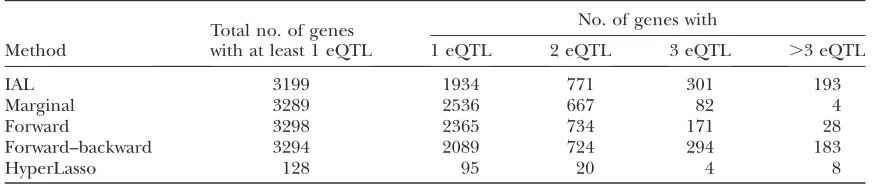
0:05=412=2Þ, and the ‘‘shape’’ parameter is set to be 1. The IAL and stepwise regressions have similar power to identify the genes with at least one eQTL (Table 1). Apparently, the IAL is the most powerful method in terms of identifying multiple eQTL per gene, and the HyperLasso has least power to identify either single eQTL or multiple eQTL per gene (Table 1).
Next we focus on the results of the IAL. Many previous studies have identified one-dimensional (1-D) eQTL hotspots. A 1-D eQTL hotspot is a genomic locus that harbors the eQTL of several genes. Similarly, if the expressions of several genes are associated with the samekloci, thesekloci are referred to as ak-D eQTL hotspot. The results of the IAL reveal several 1-D eQTL hotspots (Figure 5), as well as many eQTL hotspots of higher dimensionality. We illustrate the 2-D eQTL
hotspots in a two-dimensional plot where one point corresponds to one 2-D eQTL and thex,ycoordinates of the point are the locations of the two eQTL (Figure 6). Comparing Figures 5 and 6, it is interesting that a 1-D eQTL can be further divided into several groups on the basis of the results of 2-D eQTL, which is consistent with the finding of Zhanget al.(2010).
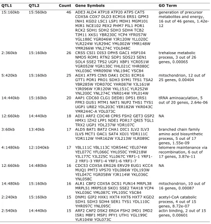
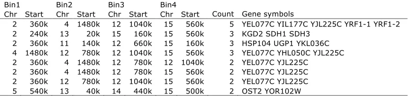
We divide the whole yeast genome into 600 bins of 20-kb regions, which lead to 6003 599/2¼179,700 bin pairs as potential ‘‘2-D eQTL hotspots’’. Eleven bin pairs are linked to.15 genes (Table S1). The cutoff is chosen arbitrarily so that we can focus on a relatively small group of 2-D hotpots with definite significant enrich-ment. Due to space limits, we discuss in detail only the largest 2-D hotspot located at chromosome (Chr)15, 160–180 kb and Chr15, 560–580 kb. There are 46 genes linked to these two loci simultaneously, and among them 16 are involved in ‘‘generation of precursor metab-olites and energy’’ (P-value 3.6031013). A closer look reveals that 41 of the 46 genes are linked to one marker block at Chr15, 170,945–180,961 bp, and one marker at Chr15, 563,943 bp. One potential causal gene nearby Chr15, 171–181 kb is PHM7 (Zhuet al.2008), and one potential causal gene nearby Chr15, 564 kb is CAT5
(Yvertet al.2003). Interestingly, both PHM7 and CAT5
are among the 46 genes linked to both loci.
There are also several cases that one group of genes linked to three loci (35.8 million possible three-loci combinations,Table S2) or even four loci (5.3 billion possible four-loci combinations, Table S3). For exam-ple, three genes, KGD2, SDH1, and SDH3 are all linked to four loci: Chr2, 240–260 kb; Chr13, 20–40kb; Chr15, 160–180 kb; and Chr15, 560–580 kb. Interestingly, all three genes are involved in an ‘‘acetyl-CoA catabolic process’’ (P-value 1.933107).
DISCUSSION
In this article, we proposed two variable selection methods, namely the BAL and the IAL. These two methods extend the adaptive Lasso in the sense that they do not require any informative initial estimates of the regression coefficients. The BAL is implemented by MCMC. Through extensive simulations, we observe the BAL has apparently better variable selection
perfor-TABLE 1
The number of genes with a certain number of eQTL
Method
Total no. of genes with at least 1 eQTL
No. of genes with
1 eQTL 2 eQTL 3 eQTL .3 eQTL
IAL 3199 1934 771 301 193
Marginal 3289 2536 667 82 4
Forward 3298 2365 734 171 28
Forward–backward 3294 2089 724 294 183
HyperLasso 128 95 20 4 8
mance than the Bayesian Lasso, slightly better perfor-mance than the Bayesiant, and slightly worse perfor-mance than the CMSA. The IAL, which is an ECM algorithm, aims at finding the mode of the posterior distribution. The IAL has uniformly the best variable performance among all the 10 methods we tested. Coupled with a variable filtering step, type I error of the IAL can be explicitly controlled.
The IAL differs from the HyperLasso (Griffin and Brown 2007; Hoggart et al. 2008) in at least two aspects. First, the HyperLasso specifies inverse gamma distribution forkj2/2, and the resulting unconditional posterior relies on a numerical function. In contrast, we specify inverse gamma distribution forkj, and it has a much simpler unconditional posterior (Equation 7). The difference is not trivial since it leads not only to convenient theoretical studies in Theorem 1 (File S1, Section C), but also to better numerical stability. For example, the HyperLasso becomes unstable for small shape parameter while IAL is stable for all possible values ofdandt. Second, we selectdandtby BIC and further filter out covariates with insignificant effects. In contrast, the HyperLasso directly assigns a large penal-ization to control the type I error. As shown in theResults section, the strong penalization of HyperLasso leads to little power to detect relatively weaker signals.
The IAL is computationally very efficient. For example, it takes 4 hr to carry out the multiple-loci mapping for the yeast eQTL data with 6100 genes and 1017 markers. In
contrast, marginal regression, forward regression, and forward–backward regression take60, 100, and 200 hr. All of the computation was done using a Dual Xenon 2.0-Ghz Quadcore server. One additional computational advantage of the IAL is that the type I error is controlled by the computationally efficient variable filtering step. The IAL results can be reused for different type I errors. In contrast, for the stepwise regression, all the computa-tion needs to be redone for each type I error.
Our results seem to contradict the results of Yiand Xu (2008) that the Bayesian Lasso has adequate variable selection performance. This inconsistency can be ex-plained by the fact that we are studying the variable selection problem with a much denser marker map. It is known that the Lasso does not have variable selection consistency if there are strong correlations between the covariates with zero and nonzero coefficients (Zou 2006). Since the Bayesian Lasso has similar penalization characteristics to the Lasso (Parkand Casella2008) and the denser marker map leads to higher correlations among genotype profiles, it is not surprising that the Bayesian Lasso has inferior performance in our simu-lations. In fact, in our simulations, the Bayesian Lasso overpenalizes the regression coefficients (Figure S8). This is consistent with the findings that ‘‘Lasso has had to choose between including too many variables or overshrinking the coefficients’’ (Radchenkoand James 2008, p. 1310). In contrast, the Bayesiant, the BAL, and the IAL have increasingly smaller penalization on the
Figure5.—Illustration of the eQTL mapping results in 112 yeast segregants. In the top panel, each point corresponds to a 1-D eQTL result, where the x-coordinate is the location of the eQTL and the y-coordinate is the location of the gene. Different colors indicate different sizes of the regression coefficients. The diagonal band indicates thecis-eQTL, where expression of one gene is associated with the genotype of a nearby marker. The vertical bands indicate 1-D eQTL hotspots. In the bottom panel, the number of genes linked to each marker is plotted. Several 1-D eQTL hotspots are apparent for those markers that harbor the eQTL of hundreds of genes.
coefficients estimates. The IAL seems to provide un-biased coefficient estimates. This leads to an assumption that the IAL has the oracle property, which warrants further theoretical study.
Due to the computational cost and the need to further filter out false discoveries, the Bayesian shrink-age methods are less attractive for large-scale computa-tion such as eQTL studies. However, there is room to improve these Bayesian shrinkage methods, such as the equi-energy sampler approach (Kouet al.2006). Alter-native prior distribution for hyperparmeters may also lead to better variable selection performance of the BAL. These strategies are among our future studies. Specifically, for the gamma prior in the BAL, we have tried the strategy to set the hyperparametersdandtas fixed numbers. In general, the results are not very sensitive to the choices ofdandt, and no combination of d and t leads to significantly better results than assigning the joint prior fordandt;i.e.,p(d,t)}t1.
In the current implementation, we handle missing genotype data by imputing them first (using the Viterbi algorithm implemented in R/qtl) and then taking the imputed values as known. A more sophisticated approach for the BAL is to take the genotype data as unknown and sample them within MCMC; and for the IAL, we can summarize its results across multiple imputations (Sen and Churchill 2001). However, these sophisticated approaches are computationally more intensive and are mainly designed for relatively sparse marker maps. The current density SNP arrays often have
high-confidence genotype call rates.98% (Rabbeeand Speed 2006). Imputation methods are also an active research topic. Haplotype information from related or unrelated individuals can be used to obtain accurate genotype imputation (Marchini et al. 2007). Therefore simply imputing the genotype data and then taking it as known may be sufficient for many studies using high-density SNP arrays, although careful examination of missing data patterns is always important.
We have mainly discussed our method in a linear regression framework. Extension to the generalized linear model (e.g., logistic regression for binary re-sponses) is possible. The generalized linear model can be solved by iterated reweighted least squares. Similar to the approach used in Friedmanet al.(2009), our method can be plugged in to solve the least-squares problem within the loop of iterated reweighted least squares. However, this approach is computationally intensive. Yi and Banerjee (2009) proposed an intriguing and effi-cient EM algorithm for multiple-loci mapping by gener-alized linear regression. In their EM algorithm, many correlated covariates can be simultaneously updated, which has the advantage of accommodating the correla-tion among the covariates. However, our method uses a different model setup and cannot adopt the same approach of Yiand Banerjee (2009). Computationally efficient extension of our method to a generalized linear model warrants further studies.
We tested the robustness of our methods by addi-tional sets of simulations where the traits are log or
Figure6.—The distribution of the locus pairs linked to the same gene. Here each point corre-sponds to a 2-D eQTL, and the background color reflects the density of the distribution. If the ex-pression of one gene is linked to more than two loci, we plot each pair of linked loci. For exam-ple, if one gene is linked to three markers 1, 2, and 3, which are located at positions p1, p2, and p3, respectively, this gene corresponds to three points in the figure, (p1,p2), (p1,p3), and (p2,p3).
exponentially transformed (results not shown). The conclusion is that our methods are robust to mild violations of linearity assumption. However, we still expect that the additive linear model assumption is severely violated in some situations,e.g., when epistatic interactions are present. As mentioned in the Introduc-tion, we can include pairwise interactions in our model, similar to the approaches used by Zhangand Xu(2005) and Yiet al.(2007). In practice, prioritizing interactions by the significance of main effects or biological knowl-edge may help to reduce the multiple-testing burden and to improve the power. How to penalize the in-teraction term also warrants further study. Grouping the interaction terms and the corresponding main effects together and applying group penalties (Yuanand Lin 2006) may be a better approach than penalizing the main effects and interactions separately.
In summary, we have developed iterative adaptive penalized regression methods for genomewide multiple-loci mapping problems. Both theoretical justifications and empirical evidence suggest that our methods have superior performance than the existing methods. Al-though our work is motivated by genetic data, our methods are general enough to be applied to other HDLSS problems.
The authors thank two anonymous reviewers and the associate editor for their constructive comments and suggestions. The authors also thank Jun Liu for his valuable suggestions for the implementation of the Bayesian adaptive Lasso. This research was supported by National Institute of Mental Health (NIMH) grants 1 P50 MH090338-01 and 1 RC2 MH089951-01. J. G. Ibrahim’s research was partially supported by National Institutes of Health (NIH) grants GM70335 and CA74015. F. Zou’s research was partially supported by NIH grant GM074175-03.
LITERATURE CITED
Brem, R. B., and L. Kruglyak, 2005 The landscape of genetic
com-plexity across 5,700 gene expression traits in yeast. Proc. Natl. Acad. Sci. USA102(5): 1572–1577.
Brem, R. B., J. D. Storey, J. Whittle and L. Kruglyak,
2005 Genetic interactions between polymorphisms that affect gene expression in yeast. Nature436(7051): 701–703.
Broman, K. W., and T. P. Speed, 2002 A model selection approach
for the identification of quantitative trait loci in experimental crosses. J. R. Stat. Soc. Ser. B64:641–656.
Broman, K. W., H. Wu, S. Senand G. A. Churchill, 2003 R/qtl:
QTL mapping in experimental crosses. Bioinformatics 19: 889–890.
Chen, J., and Z. Chen, 2008 Extended Bayesian information criteria for
model selection with large model spaces. Biometrika95(3): 759. Churchill, G., and R. Doerge, 1994 Empirical threshold values for
quantitative trait mapping. Genetics138:963–971.
Doerge, R., and G. Churchill, 1996 Permutation tests for multiple
loci affecting a quantitative character. Genetics142:285–294. Fan, J., andR. Li, 2001 Variableselection via nonconcavepenalized
like-lihood and its oracle properties. J. Am. Stat. Assoc.96:1348–1360. Friedman, J., 2008 Fastsparse regression and classification.
Techni-cal report, Stanford University, Stanford, CA.
Friedman, J., T. Hastieand R. Tibshirani, 2009 Regularization
paths for generalized linear models via coordinate descent. Tech-nical report, Department of Statistics, Stanford University, Stan-ford, CA.
George, E., and R. McCulloch, 1993 Variable selection via Gibbs
sampling. J. Am. Stat. Assoc.88:881–889.
Griffin, J., and P. Brown, 2007 Bayesian adaptive lassos with
non-convex penalization. Technical Report, University of Kent, Kent, UK.
Hans, C., 2009 Bayesian lasso regression. Biometrika96:1–11.
Hoggart, C., J. Whittaker, M. De Iorio and D. Balding,
2008 Simultaneous analysis of all SNPs in genome-wide and re-sequencing association studies. PLoS Genet.4(7):e1000130. Hoh, J., and J. Ott, 2003 Mathematical multi-locus approaches to
localizing complex human trait genes. Nat. Rev. Genet.4:701–709. Huang, J., S. Maand C.-H. Zhang, 2008 Adaptive Lasso for sparse
high-dimensional regression models. Stat. Sin.18:1603–1618. Kou, S., Q. Zhouand W. Wong, 2006 Equi-energy sampler with
ap-plications in statistical inference and statistical mechanics. Ann. Stat.34(4): 1581–1619.
Manichaikul, A., J. Moon, S. Sen, B. Yandell and K. Broman,
2009 A model selection approach for the identification of quantitative trait loci in experimental crosses, allowing epistasis. Genetics181:1077–1086.
Marchini, J., B. Howie, S. Myers, G. McVeanand P. Donnelly,
2007 A new multipoint method for genome-wide association studies by imputation of genotypes. Nat. Genet.39:906–913. Meng, X.-L., and D. B. Rubin, 1993 Maximum likelihood estimation
via the ECM algorithm: a general framework. Biometrika80(2): 267–278.
Park, T., and G. Casella, 2008 The Bayesian Lasso. J. Am. Stat.
Assoc.103:681–686.
Rabbee, N., and T. Speed, 2006 A genotype calling algorithm for
af-fymetrix SNP arrays. Bioinformatics22:7–12.
Radchenko, P., and G. M. James, 2008 Variable inclusion and
shrinkage algorithms. J. Am. Stat. Assoc.103:1304–1315. Richardson, S., and P. J. Green, 1997 On Bayesian analysis of
mix-tures with an unknown number of components (with discus-sion). J. R. Stat. Soc. Ser. B59:731–792.
Sen, S., and G. Churchill, 2001 A statistical framework for
quan-titative trait mapping. Genetics159:371–387.
Sun, W., and F. A. Wright, 2010 A geometric interpretation of the
per-mutation p-value and its application in eQTL studies. Ann. Appl. Stat. (in press). (http://www.bios.unc.edu/wsun/research.htm). Tibshirani, R., 1996 Regression shrinkage and selection via the
Lasso. J. R. Stat. Soc Ser. B.58:267–288.
Troyanskaya, O., M. Cantor, G. Sherlock, P. Brown, T. Hastie
et al., 2001 Missing value estimation methods for DNA micro-arrays. Bioinformatics17(6): 520–525.
Wasserman, L., and K. Roeder, 2009 High dimensional variable
selection. Ann. Stat.37(5A): 2178.
Yi, N., 2004 A unified Markov chain Monte Carlo framework for
mapping multiple quantitative trait loci. Genetics167:967–975. Yi, N., and S. Banerjee, 2009 Hierarchical generalized linear models
for multiple quantitative trait locus mapping. Genetics181(3): 1101. Yi, N., and S. Xu, 2008 Bayesian LASSO for quantitative trait loci
mapping. Genetics179:1045–1055.
Yi, N., D. Shriner, S. Banerjee, T. Mehta, D. Pompet al., 2007 An
ef-ficient Bayesian model selection approach for interacting quanti-tative trait loci models with many effects. Genetics176:1865–1877. Yuan, M., and Y. Lin, 2006 Model selection and estimation in
regres-sion with grouped variables. J. R. Stat. Soc. Ser. B68(1): 49–67. Yvert, G., R. B. Brem, J. Whittle, J. M. Akey, E. Foss et al.,
2003 Trans-acting regulatory variation in Saccharomyces cerevi-siae and the role of transcription factors. Nat. Genet.35(1): 57–64. Zhang, W., J. Zhu, E. E. Schadtand J. S. Liu, 2010 A Bayesian
par-tition method for detecting pleiotropic and epistatic eQTL mod-ules. PLoS Comput. Biol.6(1): e1000642.
Zhang, Y., and S. Xu, 2005 A penalized maximum likelihood method
for estimating epistatic effects of QTL. Heredity95:96–104. Zhu, J., B. Zhang, E. Smith, B. Drees, R. Bremet al., 2008 Integrating
large-scale functional genomic data to dissect the complexity of yeast regulatory networks. Nat. Genet.40(7): 854.
Zou, H., 2006 The adaptive Lasso and its oracle properties. J. Am.
Stat. Assoc.101:1418–1429.
Zou, H., and R. Li, 2008 One-step sparse estimates in nonconcave
penalized likelihood models. Ann. Stat.36:1509–1533. Zou, H., T. Hastieand R. Tibshirani, 2007 On the ‘‘degrees of
freedom’’ of the lasso. Ann. Stat.35(5): 2173–2192.
Supporting Information
http://www.genetics.org/cgi/content/full/genetics.109.114280/DC1
Genomewide Multiple-Loci Mapping in Experimental Crosses
by Iterative Adaptive Penalized Regression
Wei Sun, Joseph G. Ibrahim and Fei Zou
W. Sun et al.
2 SI
Supplementary Materials for “Genome-wide Multiple Loci
Map-ping in Experimental Crosses by the Iterative Adaptive Penalized
Regression” by Wei Sun, Joseph G. Ibrahim and Fei Zou
A: The Gibbs Sampler for the Bayesian adaptive Lasso
1. Initialization. We initialize (b0, b1, ..., bp) with zero and initialize (σ
2e
,
κ1, ...,
κp)
with a positive number.
2. Update
b
0: Let
Θ
−parameter1denote all of the parameters except parameter
1.
The conditional posterior distribution of
b
0is
p(b
0|
Θ
−b0)
∼
N(¯
b
0, s
2
0
),
(1)
where ¯
b0
= (1/n)
!
n1(yi
−
!
pj=1xijbj), and
s
20= (1/n)σ
e2.
3. Update
b
j: The conditional posterior distribution of
b
jis
p(bj
|
Θ
−bj)
∝
exp
"
−
(b
j−
¯
bj)
2
2σ
2 j−
|
b
j|
κj
#
,
(2)
where
σ
j2=
σ
2 e!
ni=1
x
2ij, and ¯
bj
=
$
n%
i=1
x
2ij&
−1 n%
i=1
xij
$
yi
−
b0
−
%
k"=j
xikbk
&
.
(3)
Although
p(bj
|
Θ
−bj) has no closed form, it is log-concave. Thus we sample
bj
by Adaptive Rejection Sampling (ARS) [Gilks, 1992]. Note that whenever one
of the
b
j’s is updated, it is used immediately for updating the other
b
j’s.
4. Update
σ
2 e:
p(σ
2 e|
Θ
−σ2e
)
∝
(σ
2e
)
−1−n/2exp
'
−
rss
/(2σ
2 e)
(
,
(4)
which is inv-Gamma(σ
2e
;
n/2,
rss
/2).
1
FILE S1
Supporting Information
W. Sun et al. 3 SI
5. Update
κ
j:
p
(κ
j|
Θ
−κj)
∝
κ
− 2−δj
exp
!
−
|
b
j|
+
τ
κ
j"
,
(5)
which is inv-Gamma(κ
j; 1 +
δ
,
|
b
j|
+
τ).
6. Update
τ
:
p
(τ
|
Θ
−τ)
∝
τ
pδ−1exp
#
−
τ
p
$
j=1
κ
−j1%
.
(6)
Therefore
τ
|
Θ
−τ∼
Gamma(
p
δ
,
&
pj=1κ
−j1).
7. Update
δ:
p
(δ
|
Θ
−δ)
∝
#
τ
p'
p j=1κ
j%
δΓ
(δ)
−p.
(7)
It is easy to show that
p
(δ
|
Θ
−δ) is log-concave, so we sample
δ
using ARS.
B: Derivations of Iterative Adaptive Lasso
CM step of the iterative adaptive Lasso
As shown in Section A, the conditional posterior distribution of
b
jis
p
(
b
j|
Θ
−bj)
∝
exp
(
−
(
b
j−
¯
b
j)
2
2σ
2j
−
|
b
j|
κ
j)
,
(8)
where
σ
2j=
σ
2e
&
n i=1x
2ij, and ¯
b
j=
#
n$
i=1
x
2ij%
−1 n$
i=1
x
ij#
y
i−
b
0−
p
$
k"=j
x
ikb
k%
.
(9)
Let
ζ
jbe the mode of the conditional posterior distribution of
b
j, then
ζ
j= arg min
bjf
(
b
j),
where
f
(
b
j) = (
b
j−
¯
b
j)
2/
(2σ
2j) +
|
b
j|
/
κ
j. Therefore
ζ
jcan be solved by letting the
2
W. Sun et al.
4 SI
derivative of
f(b
j) to be 0. One extra complexity arises because the derivative of
|
b
j|/
κ
jdoes not exist at
b
j= 0. This problem can be circumvented by considering
three situations: ¯
bj
>
0, ¯
bj
= 0, and ¯
bj
<
0. It is easy to show that
ζ
j= 0
if ¯
bj
= 0
ζ
j∈
[0,
¯
b
j] if ¯
b
j>
0
ζ
j∈
[¯
b
j,
0] if ¯
b
j<
0
.
•
If ¯
bj
>
0, we can first consider the derivatives of
f
(bj) in (0,
¯
bj]:
f
!(bj) =
b
j/
σ
2j−
¯
b
j/
σ
j2+ 1/
κ
j, and
f
!!(b
j) = 1/
σ
j2. If ¯
b
j≤
σ
2j/
κ
j,
f
!(b
j)
>
0, therefore
f(bj) may achieve its minimum at 0. This is can be proved as follows.
–
If 0
<
¯
b
j≤
σ
2j/
κ
j,
∀
b
j∈
[0,
¯
b
j]
f(b
j)
−
f(0) = (b
j−
¯
b
j)
2/(2
σ
2j) +
|
b
j|/
κ
j−
¯
b
2j/(2
σ
2j) =
b
2j/(2
σ
2j)
−
b
j¯
b
j/
σ
2j+
b
j/
κ
j=
b
2j/(2
σ
2j) + (bj/
σ
j2)(
σ
2j/
κ
j−
¯
bj)
≥
0,
therefore
ζ
j= 0.
–
If ¯
b
j>
σ
2j/
κ
j, when
b
j= ¯
b
j−
σ
j2/
κ
jf
!(b
j) = 0, and
f
!!(b
j)
>
0. Therefore
ζ
j= ¯
bj
−
σ
j2/
κ
j•
If ¯
b
j<
0, similar to the situation of ¯
b
j>
0, we can first consider the derivatives
of
f(bj) in [¯
bj,
0):
f
!(bj) =
bj/
σ
2j
−
¯
bj/
σ
j2−
1/
κ
j, andf
!!(bj) = 1/
σ
j2. If ¯
bj
≥
−
σ
2j
/
κ
j,
f
!(b
j)
<
0, therefore
f(b
j) may achieve its minimum at 0. This is can
be proved as follows:
–
If
−
σ
2j
/
κ
j≤
¯
b
j<
0,
∀
b
j∈
[¯
b
j,
0]
f(b
j)
−
f(0) = (b
j−
¯
b
j)
2/(2
σ
2j) +
|
b
j|/
κ
j−
¯
b
2j/(2
σ
2j) =
b
2j/(2
σ
2j)
−
b
j¯
b
j/
σ
2j−
b
j/
κ
j=
b
2j/(2
σ
2j)
−
(b
j/
σ
2j)(¯
b
j+
σ
2j/
κ
j)
≥
0,
therefore
ζ
j= 0.
–
If ¯
b
j<
−
σ
j2/
κ
j, when
b
j= ¯
b
j+
σ
j2/
κ
jf
!(b
j) = 0, and
f
!!(b
j)
>
0. Therefore
ζ
j= ¯
b
j+
σ
2j/
κ
j3
W. Sun et al. 5 SI
Summarizing the above results, we have
ζj
= 0
if
−
σ
2j
/κj
≤
¯
bj
≤
σ
j2/κj
ζj
= ¯
bj
−
σ
2j
/κj
if ¯
bj
>
σ
j2/κj
ζj
= ¯
bj
+
σ
2j
/κj
if ¯
bj
<
−
σ
j2/κj
.
Note that this CM-step update is actually quite similar to the shooting method for
the Lasso calculation [Fu, 1998].
E-step of the iterative adaptive Lasso
The complete data log-posterior is
l
(
θ
|
y
,
X
,
φ
) =
C
−
rss
/
(2
σ
2 e)
−
p
$
j=1
|
b
j|κj
,
(10)
where
C
is a constant with respect to
θ
. Suppose in the
t
-th iteration, the parameter
estimates are
θ
(t)= (
b
(t)0
, b
(t) 1, ..., b
(t)
p
). Then the conditional expectation with respect
to the conditional density of
f
(
φ
|
y
,
X
,
θ
(t)) is
Q
(
θ
|
θ
(t)) =
%
l
(
θ
|
y
,
X
,
φ
)
f
(
φ
|
y
,
X
,
θ
(t))
dφ
=
% &
C
−
rss
/
(2
σ
2 e)
−
p
$
j=1
|
b
j|κj
'
f
(
φ
|
y
,
X
,
θ
(t))
dφ.
(11)
From the derivation of the Bayesian adaptive Lasso, we have
f
(
φ
|
y
,
X
,
θ
(t)) =
C
fσ
2+ne
exp
(
−
rss
(t)/
(2
σ
2 e)
)
*
pj=1
κ
−2−δj
exp
&
−
|
b
(t) j
|
+
τ
κj
'
,
(12)
where
rss
(t)is the residual sum of squares calculated using
θ
(t),
C
f
is the normalizing
constant. By letting
+
f
(
φ
|
y
,
X
,
θ
(t))
dφ
= 1, it is easy to show that
C
f=
,
1
Γ(
n/
2)
(
rss
(t)/
2
)n/2
-
p
*
j=1