ABSTRACT
SU, LIN. New Estimation and Decision-making Methods for Correlated and Network Data. (Under the direction of Wenbin Lu and Howard Bondell.)
Study of correlated data is of great interest in Statistics. Numerous methods have
been proposed to handle correlation in different scenarios. Among all the practical fields
that correlated data arises, network data has drawn much attention in recent years,
which requires new statistical models to address the interaction between subjects. In
this thesis, we firstly propose new estimation methods for the regular correlation issue in
linear regression, and then we focus on the estimation and decision-making problems in
network data.
In Chapter 2, we propose methods to construct a biased linear estimator for
lin-ear regression which optimizes the relative mean squared error (MSE). Although there
have been proposed biased estimators for correlated data that are shown to have better
performance than the ordinary least squares (OLS) estimator in terms of MSE, our
con-struction is based on the minimization of relative MSE directly. The performance of the
proposed methods are illustrated by a simulation study and a real data example. The
results show that our methods can improve on MSE when there exists correlation among
the predictors.
In Chapter 3, we focus on the time-to-event data in the presence of network
correla-tion. We are interested in whether people’s responses to an event are affected by their
friends’ characteristics. Studying social network dependence is an emerging research area.
We propose a novel latent Cox model with contextual effect. The proposed model
intro-duces a latent indicator to characterize whether a person’s survival time might be affected
exis-tence of social network dependence. If it exists, we further develop an EM-type algorithm
to estimate the model parameters. The performance of the proposed test and estimators
are illustrated by simulation studies and an application to a time-to-event data set of a
mobile game network data.
In Chapter 4, we address the decision-making problem with network interference. In
many network-based intervention studies, treatment applied on an individual or his/her
own characteristics may also affect the outcome of other connected people. We call this
interference along network. Approaches for deriving the optimal individualized treatment
regime remain unknown after introducing the effect of interference. We propose a novel
network-based regression model that is able to account for interaction between outcomes
and treatments in a network. Both Q- and A-learning methods are derived. We show that
the optimal treatment regime under our model is independent from interference, which
makes its application in practice more feasible and appealing. The asymptotic properties
of the proposed estimators are established. The performance of the proposed model and
methods are illustrated by extensive simulation studies and an application to the same
© Copyright 2018 by Lin Su
New Estimation and Decision-making Methods for Correlated and Network Data
by Lin Su
A dissertation submitted to the Graduate Faculty of North Carolina State University
in partial fulfillment of the requirements for the Degree of
Doctor of Philosophy
Statistics
Raleigh, North Carolina
2018
APPROVED BY:
Rui Song Eric Chi
Wenbin Lu
Co-chair of Advisory Committee
Howard Bondell
DEDICATION
BIOGRAPHY
The author was born in May 1990 in Dalian, a beautiful coastal city in the northeast
of China. She lived there till graduating from Dalian No.24 High school. In 2009, Lin
attended the School of Mathematical Sciences at Nankai University in Tianjin, China.
After graduating with a B.S degree in Statistics in 2013, she moved to the U.S and joined
the Department of Statistics at North Carolina State University. Under the direction of
ACKNOWLEDGEMENTS
First of all, I would like to express my deepest appreciation to my advisors, Dr. Wenbin
Lu and Dr. Howard Bondell, for their guidance, knowledge and support. They taught me
how to conduct statistical research from the very beginning. They helped me overcome
the obstacles every time I struggled. They were so considerate and patient whenever
I encountered any difficulty. I am consistently inspired by their passion and curiosity,
which will have a prolonged influence on my future work. I feel very lucky and honored
to be their student. I would also like to thank Dr. Rui Song, who actively collaborated in
this work. I enjoyed meeting with her almost every week. Her insightful comments and
suggestions enormously helped me in research. I am also fortunate to have Dr. Eric Chi
on my committee. His constructive comments improved this work. I really appreciate Dr.
Shih-Chun Lin and Dr. Kevin Potter, who agreed to serve on my committee despite their
busy schedule.
There are many faculty members and staff in the department I would like to express
my gratitude, without whom I would not come so far. Special thanks to Dr. John
Mon-ahan, who sent me the offer five years ago so that I had the opportunity to continue my
study at NC State. I am grateful to all the faculty members who provided various
excel-lent courses that solid my foundation and broaden my horizon. Their profound knowledge
and enthusiasm in Statistics motivate me to learn more and more. I also enjoyed working
with all the professors as their teaching assistant. They always trust and support me. I
would like to thank all DGPs, for their patience in answering me all kinds of questions
and signing numerous forms. Thank Dr. Dennis Boos for randomly chatting with me
about life, Dr. Charles Smith for holding many interesting events in the department,
have found myself in the Ph.D program at NC State without my teachers at Nankai
University, who led me to the world of Mathematics and Statistics.
I feel so lucky to have all the talented friends and classmates around me in the past
years. Jennifer, my lovely best friend and officemate, shares all the happiness and
frustra-tion in life and work with me. I also benefited a lot from discussions with my classmates
on coursework and research, especially Wenhao, Marshall, Liuyi, and Chengchun. I
ap-preciate the help from many alumni of the department, who generously shared their
experience and tried their best to help me, such as Anran, Teng, Peng, Yingzi and Zhou.
I am also grateful to the valuable industrial internship experiences at GSK and
Ama-zon. Special thanks go to my amazing supervisors, Katja, Mandy, Guang and Lucas.
They helped me have a deeper understanding on the application of Statistics in practice.
They taught me many precious skills as a statistician in the real world, such as how to
communicate effectively as a consultant, how to write more readable and reproducible
code, and how to write clear and attracting documentation.
Most importantly, I want to thank my family for their unconditional love. My parents
provided the best possible environment and opportunity for my development. They keep
encouraging me to believe in myself and be brave to explore the unknown world. I am
especially grateful for their support five years ago when I decided to continue my study
on the other side of the world. I appreciate NC State a lot because I met my husband,
Shaobo Cai, here. He shares all the ups and downs with me in the past years. No matter
what happens, he always gives me the strongest support. I could not be too grateful to
TABLE OF CONTENTS
LIST OF TABLES . . . viii
LIST OF FIGURES . . . ix
Chapter 1 Introduction . . . 1
1.1 Classic Methods for Correlated Data in Linear Regression . . . 2
1.2 Types of Network Dependence . . . 3
1.3 Recent Development for Network Data Analysis . . . 5
1.4 Outline . . . 7
Chapter 2 Best Linear Estimation via Minimization of Relative Mean Squared Error . . . 8
2.1 Introduction . . . 8
2.2 Optimal Linear Biased Estimator . . . 10
2.2.1 Preliminaries . . . 10
2.2.2 Full Minimization . . . 11
2.2.3 Partial Minimization . . . 12
2.3 Simulation Study . . . 17
2.4 Pyrimidine Data . . . 20
2.5 Discussion . . . 21
Chapter 3 Testing and Estimation of Social Network Dependence with Time to Event Data. . . 27
3.1 Introduction . . . 27
3.2 Latent Cox Model with Contextual Effect . . . 29
3.3 Testing and Estimation Methods . . . 31
3.3.1 Test forH0 :ρ= 0 . . . 31
3.3.2 Parameter Estimation . . . 34
3.4 Simulation Studies . . . 38
3.4.1 Simulation Results for Testing . . . 39
3.4.2 Simulation Results for Estimation . . . 40
3.5 An Application: Tencent QQ Game Data . . . 42
3.6 Discussion . . . 45
Chapter 4 Q- and A-learning Methods for Optimal Treatment Decision with Interference . . . 49
4.1 Introduction . . . 49
4.2 Q-learning . . . 51
4.2.2 Model Fitting . . . 54
4.3 A-learning . . . 55
4.3.1 Model Formulation . . . 55
4.3.2 Model fitting . . . 56
4.4 Simulation Studies . . . 57
4.5 Application to Tencent QQ Game Data . . . 60
4.6 Conclusions . . . 61
References . . . 66
Appendices . . . 74
Appendix A . . . 75
A.1 Proof of Theorem 1 . . . 75
A.2 Proof of Proposition 1 . . . 77
A.3 Proof of Theorem 2 . . . 78
Appendix B . . . 80
B.1 Proof of Theorem 3 . . . 80
B.2 Proof of Theorem 4 . . . 81
B.3 Calculation of ∇2g( ˆΘ|Θˆ) . . . . 85
Appendix C . . . 86
C.1 Proof of Theorem 5 . . . 86
LIST OF TABLES
Table 2.1 Mean Squared Prediction Errors (MSPE) for the Pyrimidine Data . . 22
Table 3.1 Type I error and power of the proposed test. . . 40
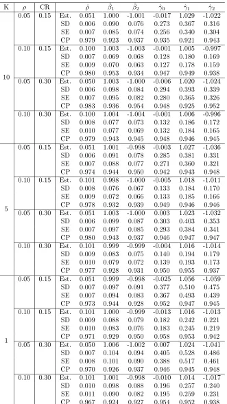
Table 3.2 Simulation results for parameter estimation. . . 41
Table 3.3 Analysis results for Tencent QQ game data. . . 43
Table 3.4 Analysis results of simplified model (3.10) for Tencent QQ game data. 45 Table 4.1 Q-learning simulation results. . . 63
Table 4.2 A-learning simulation results. . . 64
Table 4.3 Q-learning results for Tencent QQ game data. . . 64
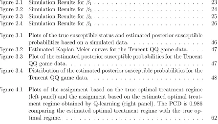
LIST OF FIGURES
Figure 2.1 Simulation Results for β1 . . . 23
Figure 2.2 Simulation Results for β2 . . . 24
Figure 2.3 Simulation Results for β3 . . . 25
Figure 2.4 Simulation Results for β4 . . . 26
Figure 3.1 Plots of the true susceptible status and estimated posterior susceptible probabilities based on a simulated data. . . 46
Figure 3.2 Estimated Kaplan-Meier curves for the Tencent QQ game data. . . . 47
Figure 3.3 Plot of the estimated posterior susceptible probabilities for the Tencent QQ game data. . . 47
Figure 3.4 Distribution of the estimated posterior susceptible probabilities for the Tencent QQ game data. . . 48
Chapter 1
Introduction
Statistical study in the presence of correlation or dependence between subjects is always
of great interest. In general, correlation can come from various sources and belongs to
different types. In linear regression, high correlation between predictors is a common
con-cern, which can cause tremendously high variance of the ordinary least square estimator.
Therefore, various estimators have been proposed to handle such multicollinearity, which
usually yield smaller mean squared error. We are interested in proposing new estimation
methods for correlated data that can minimize the mean squared error directly. Another
type of correlation arises when influence between friends is ineligible. Dependence
be-tween friends is an emerging research area. When considering the network effect, classic
statistical models can no longer characterize the features of data. Therefore, there
ap-pears a huge demand of new methods for correlated and network data in all traditional
statistical fields. In particular, we are interested in time-to-event responses and
decision-making methods with network dependence into consideration. We want to address two
problems. Firstly, if the time that people response to an event is affected by their friends,
response is affected by his/her friends, what is the optimal decision in order to optimize
it? In this chapter, we give a brief review of the classic estimators for correlated data in
linear regression and recent developments in studying network dependence.
1.1
Classic Methods for Correlated Data in Linear
Regression
Consider the multiple linear regression model,
y=Xβ+, (1.1)
where y and are n ×1 vectors, X is a n×p matrix, β is a p×1 vector, and is
random withE() = 0andV ar() =σ2In. The ordinary least square (OLS) estimator is
defined as ˆβOLS = (XTX)−1XTy, which is proved to have the smallest variance among
all unbiased linear estimators by the Gauss-Markov Theorem. It is straightforward to
show that Var( ˆβOLS) = σ2(XTX)−1. SupposeXTX =QΛQT by eigen decomposition,
where Q is an orthogonal matrix and its columns are the eigenvectors. Λ is a diagonal matrix, whose elements are the eigenvalues. When two or more columns of X are highly
correlated, at least one of the diagonal elements ofΛ can be very small, which results in Var( ˆβOLS) = σ2QΛ−1QT being large. Therefore, when evaluating by the mean squared
error (MSE), which is the sum of squared bias and variance, the OLS estimator is not
ideal for correlated data.
One well-known solution is the ridge regression estimator (Hoerl and Kennard, 1970),
which is formulated as ˆβRidge= (XTX+λI)−1XTy. The extra term λI guarantees the
can be shown to outperform OLS in terms of MSE. Another interesting estimator of such
type is proposed by Liu (1993). It is given as ˆβd= (XTX+Ip)−1(XTy+dβˆOLS), where
0< d <1 is a tuning parameter. This estimator was developed to combine the advantages
of both the ridge and the James-Stein estimator. These estimators belong to the so-called
shrinkage estimators. The ridge estimator can be obtained by adding regularization to
the regular squared loss that controls the magnitude of the coefficients, so that the
estimates are shrunk to 0. Other shrinkage methods include but not restrict to the least
absolute shrinkage and selection operator (LASSO) (Tibshirani, 1996), the smoothly
clipped absolute deviation (SCAD) (Fan and Li, 2001), the elastic net (Zou and Hastie,
2005), the adaptive Lasso (Zou, 2006), etc. These estimators consider different types of
regularizations, which are all able to shrink the coefficients from the OLS estimator. It can
be presented theoretically or numerically that these estimators can result in smaller MSE
under different circumstances. However, none of these estimators are designed initially
to target at minimizing the MSE, which makes it hard to select the best estimator for a
practical correlated data set.
1.2
Types of Network Dependence
When considering the dependence between subjects in a network, it becomes more
compli-cated because the dependence can come from various aspects. As described in psychology
and economics literatures (Manski, 1993; Shalizi and Thomas, 2011), there are mainly
three types of social network dependence, namely contextual (exogenous), endogenous
(contagion) and correlated effects (external causation). Contextual effect means friends
have similar responses because they share similar characteristics. For example, friends
effect refers to the situation when one’s outcome depends on others’ outcome. For
exam-ple, I do not know what machine learning is but my friends all share the same course link
of machine learning, so I share it as well. Correlated effect exists when an external effect
results in the similarity between friends. For example, given friends usually live in the
same city, an earthquake can hurt them at the same time. Contextual and endogenous
effects are two major social network dependence people are interested in studying. In this
work, we focus on the contextual effect in our models.
Mathematically, as described by Manski (1993), in a linear regression setting, suppose
y is the response, x are some group attributes that are shared by the network, (z,u)
are individual’s attributes where u is not observed and we assume it depends on group
characteristic x. The linear model with all effects included is proposed as
y =α+βE(y|x) +γTE(z|x) +ηTz+u
and E(u|x,z) = δTx. Therefore, the mean of y given x and z is modeled as α +
βE(y|x) +γTE(z|x) +ηTz+δTx. The endogenous effect, contextual effect or correlated
effect exist when β 6= 0, γ6=0 or η6=0 respectively.
In the study of economics or psychology, researchers paid lots of efforts on
distin-guishing these effects and learning the relationship between them. In recent studies of
network in statistics, people usually do not categorize the type of dependence explicitly.
We propose our models or methods mainly for the contextual effect. Including the other
1.3
Recent Development for Network Data Analysis
In the research of social network data, the first question of interest is the network
struc-ture. Various models have been proposed to characterize it, which include but are not
limited to the stochastic block model (Wang and Wong, 1987; Nowicki and Snijders,
2001), exponential random graph model (Frank and Strauss, 1986; Hunter et al., 2008)
and latent space model (Hoff et al., 2002; Hoff, 2003; Chang et al., 2018).
It has been widely studied that people are likely to be influenced by their friends on
social network (Manski, 1993; Shalizi and Thomas, 2011; Huang et al., 2016; Zhu et al.,
2017). As described in Section 1.2, there are mainly three types of network dependence.
Multiple methods have been proposed for modeling such social network dependence. One
popular approach is to introduce a network-based penalty on individual node effects,
for example, see Li et al. (2016). In their work, a cohesion penalty similar to the graph
Laplacian regularization is posited on individual node effects, which encourages similarity
between effects of linked nodes. Similar ideas have also been widely used for building
prediction models for studying gene-network data (e.g. Li and Li, 2008, 2010; Sun et al.,
2014). Another popular approach is to consider spatial autoregression models, with the
parameter of spatial autocorrelation that quantifies the interactive dependence between
connected nodes in a network (Chen et al., 2013). The maximum likelihood estimation for
various spatial autocorrelation models have been studied in the economics literature (e.g.
Ord, 1975; Anselin, 1980; Bramoull´e et al., 2009; Lee et al., 2010). Recently, Zhou et al.
(2017) proposed several likelihood-based estimation methods for spatial autocorrelation
in a linear regression setting based on sampled network data.
In the area of network-based intervention, it is often observed that treatment of one
the coverage of vaccination in a neighborhood can affect the infection rate for an
non-vaccinated individual (Halloran and Struchiner, 1995). Getting a private tutor may affect
the grade of other students in the same study group. Encouraging users to vote on social
network can improve the voting rate among his/her friends (Bond et al., 2012). More
ex-amples can be found in Sobel (2006), Hong and Raudenbush (2006), Rosenbaum (2007),
etc. The existence of interference introduces challenges to the traditional statistical
anal-yses. In order to handle the interaction between treatments of different individuals, new
methodologies for experiment design have been developed. Related work include Basse
and Airoldi (2015) and Eckles et al. (2017). In the area of causal inference for social
network data, a common assumption is called partial interference, which basically states
that interference exists in partitioned small groups but not between different groups.
Under this framework, different types of causal inference have been studied by many
authors, for example, Hudgens and Halloran (2008), Tchetgen and VanderWeele (2012),
Aronow and Samii (2013), Liu and Hudgens (2014), Liu et al. (2016) and Sussman and
Airoldi (2017).
In this work, we address the problems of network dependence and interference from
different aspects, which are novel from previous studies. Instead of introducing the graph
regularization to the models, or inheriting the autocorrelation models, we bring in an
additive term to account for the network information, which models the contextual effect.
Besides, we deal with two different problems in the presence of network data. One is to
model the time to event data, known as survival analysis in traditional biostatistics
studies. We propose a new Cox model with the contextual effect. Another problem is to
find the optimal decision rule when interference exists. We remove the restriction of partial
interference, but propose a model with contextual effect. The attractive point of our
which makes it easy to be applied in practice.
1.4
Outline
In this dissertation, we propose several new estimation and decision-making methods
for correlated and network data. The rest of this thesis is organized as follows. Chapter
2 introduces a new biased linear estimator for linear regression, which is designed to
minimize the relative mean squared error. Details about calculation and computation
for our proposed estimator are presented. From Chapter 3, we focus on solving
network-related problems. Chapter 3 proposes a novel Cox model for network data. A score-type
test is firstly derived to test the existence of social network dependence. When it exists,
an EM-type algorithm is further developed to obtain the parameter estimation. Chapter
4 introduces new methods for optimal decision rule in the presence of interference. Both
Q- and A- learning methods are derived. Computational details are also provided. For
each chapter, sufficient simulation studies and an real data example are presented to
Chapter 2
Best Linear Estimation via
Minimization of Relative Mean
Squared Error
2.1
Introduction
Consider the linear regression model,
y=Xβ+, (2.1)
where y and are n ×1 vectors, X is a n×p matrix, β is a p×1 vector, and is
random with E() = 0 and V ar() = σ2In, where In is the n×n identity matrix. It
is well known that the ordinary least squares (OLS) estimator for β is the best linear
unbiased estimator (BLUE) based on the Gauss-Markov Theorem, in that it has minimum
where MSE( ˆβ) denotes the MSE of the estimator ˆβ and is given by
MSE( ˆβ) =E[( ˆβ−β)T( ˆβ−β)]
=[Bias( ˆβ)]T[Bias( ˆβ)] +T r(Var( ˆβ)).
Considering linear estimators, if one is willing to tolerate some bias, it is possible to
suf-ficiently reduce the variance so that the estimator achieves smaller MSE. In this chapter,
we seek to obtain an estimator that can minimize the MSE. The challenge is that MSE,
of course, depends on the true values of the parameters which are unknown in practice.
We propose two approaches to get an approximately optimal linear estimator. A natural
first approach is to minimize MSE directly via decomposing it into bias and variance and
obtaining an estimate of each quantity. Another approach is to minimize the variance for
any fixed amount of bias. This approach will lead to an estimator with smallest MSE for
any bias level. In some cases, we may have some natural tolerance for a percent bias that
we are willing to accept. In other cases, we can estimate the bias of a proposed estimator,
and can reduce its variance while matching that bias, thus obtaining an estimator with
smaller MSE than the original. To narrow the domain of candidate estimators, we only
focus on linear estimators.
The rest of this chapter is organized as follows. In Section 2.2, we introduce the
for-mulation of our estimator, and discuss the computational details. In Section 2.3, we show
simulation results and comparison between different methods under several conditions.
2.2
Optimal Linear Biased Estimator
2.2.1
Preliminaries
Consider any linear estimator
ˆ
β =M y, (2.2)
whereM is ap×nmatrix. For example, for the OLS estimator,MOLS = (XTX)−1XT;
while for the ridge estimator, Mλ = (XTX+λIp)−1XT. Under the linear model (2.1),
we have that
ˆ
β=β+ (M X−Ip)β+M .
Under the Gauss-Markov assumptions, that is,has mean0 and varianceσ2I
n, the bias
vector and variance matrix of the linear estimator in (2.2) are
Bias( ˆβ) = E( ˆβ)−β= (M X−Ip)β,
Var( ˆβ) =V ar(M ) =σ2M MT.
Consider the relative MSE of an estimator ˆβ given by
Relative MSE = E( ˆβ−β)
T( ˆβ−β)
βTβ
= [Bias( ˆβ)]
T[Bias( ˆβ)] +σ2T r(M MT)
βTβ
= β
T(M X−I
p)T(M X−Ip)β+σ2T r(M MT)
Our goal is to find a linear estimator ˆβ that has the minimum relative MSE. The main
challenge is that, in reality, the parameters β and σ2 are unknown. We propose three
methods to calculate the approximately optimal estimator introduced respectively in
Section 2.2.2, 2.2.3 and 2.2.3.
2.2.2
Full Minimization
If β and σ2 are known, minimizing the relative MSE is equivalent to minimizing the
function
f(MV) = (D0MV −β)T(D0MV −β) +σ2(MV)TMV,
where D0 = (Xβ)T ⊗Ip and MV denotes the vector obtained from vectorizing M by
column. By taking the derivative of f(MV) with respect to MV, it is straightforward to
show that the relative MSE is minimized at
c
MV = (DT0D0+σ2Inp)−1D0Tβ. (2.3)
However, the true parameters β andσ2 are unknown. A natural approach is to calculate initial estimators ˜β and ˜σ2, and plug them in (2.3). Intuitively, the performance of the
new estimator depends on the initial estimators of ˜β and ˜σ2, and it is not guaranteed
that the MSE is minimized. Note that there is no restriction on the choice of ˜β and ˜σ2
used here, that is, they can be either biased or unbiased, linear or nonlinear. We call this
method “full minimization” because the relative MSE is considered as a whole, and both
2.2.3
Partial Minimization
Note that the relative MSE can be decomposed into two parts, the bias term and the
variance term. If we allow the bias to be controlled at a constant, then the best linear
estimator with the minimum relative MSE can be found by solving
minimize
M∈Rp×n
T r(M MT)
subject to: β
T(M X−I
p)T(M X−Ip)β
βTβ ≤c, (2.4)
wherecis a constant. Supposecis the relative bias from another estimator, then we can
get a new estimator with smaller MSE when matching their bias. Methods to choose c
are discussed in Section 2.2.3. Compared to the full minimization method described in
Section 2.2.2, this optimization problem is independent of σ2, but the vector β appears
in the inequality constraint in (2.4). To get rid of the true β, we propose the following two solutions in Section 2.2.3 and Section 2.2.3.
Two-Step Optimization
As proposed in the full minimization, we can calculate an initial estimator ˜β, plug it in
(2.4) and then solve
minimize
M∈Rp×n
T r(M MT)
where c0 is a constant. Problem (2.5) can be formulated as a quadratically constrained quadratic programming (QCQP) problem. Let D= (Xβ˜)T ⊗I
p. (2.5) is equivalent to
minimize
MV∈ Rnp×1
(MV)TMV
subject to: (DMV −β˜)T(DMV −β˜)≤c0.
Because DTD is semi-positive definite, this problem is convex. Therefore, it can be solved by most convex programming software, such as Gorubi, Mosek, or CVX (Grant
and Boyd, 2014, 2008) in MATLAB.
Instead, the following theorem provides an explicit closed-form solution, and hence
the optimization problem is convenient to work with.
Theorem 1. For any n×p matrix X, and p×1 vectorβ˜, such that Xβ˜6=0, let
ˆ
M =argmin
M∈Rp×n
T r(M MT)
subject to: β˜T(M X−Ip)T(M X−Ip) ˜β ≤c0. (2.6)
Then,
ˆ
M =
(bTb)−1bT ⊗β˜ c0 = 0,
bT(1/λI
n+bbT)−1 ⊗β˜ 0< c0 <β˜Tβ˜,
0 c0 ≥β˜Tβ˜,
where b=Xβ˜, and λ= −1+
√
Pp
i=1β˜i2/c0
bTb .
the following discussion as we first calculate an initial estimator, ˜β. Similar to that in the
full minimization, there is no restriction on the estimator ˜β, and the performance of this
two-step approach depends on the performance of ˜β. Although the exact bias cannot be
strictly controlled by this two-step approach, the two-step method is likely to provide us
an estimator at least better than the initial estimator in terms of MSE.
Controlling the Worst-case Relative Bias
Suppose that the inequality (2.4) is true for ∀β ∈ Rp, then it surely holds for the true
β. So instead of dealing with the true β, we relax (2.4) to hold for ∀β ∈ Rp. Now, the
problem becomes
minimize
M∈Rp×n T r(M M
T
)
subject to: max
β∈Rp
βT(M X−I
p)T(M X−Ip)β
βTβ ≤c
∗
, (2.7)
where c∗ is a constant.
Proposition 1. The constrained optimization problem in (2.7) is equivalent to the convex semi-definite programming problem:
minimize
MV∈ Rnp×1,
t∈R1
t (2.8)
subject to:
t [MV]T
MV I np
is n.n.d,
c∗Ip (M X−Ip)T
M X−Ip Ip
where “n.n.d.” means non-negative definite.
The proof of Proposition 1 is provided in Appendix A.2. The problem described in (2.8)
is a typical semi-definite programming problem, which also is a subclass of convex
pro-gramming and can be solved by the same software mentioned in Section 2.2.3. We use the
CVX package in MATLAB. Intuitively, if the true parameter is close to the worst-case
β which gives the maximum solution to the left hand side of (2.7), this method may
provide an estimator with smaller MSE than other biased estimators after summarizing
both bias and variance. However, if not, the bias calculated by the true parameter may
be much smaller than the required upper bound. In other words, constraint (2.7) may be
overly cautious that the corresponding estimator may not be ideal. We call this approach
the worst-case controlling method in the rest of this chapter.
How to choose c0 or c∗
In some cases, we may have some natural tolerance for a percent bias that we are willing
to accept. However, in many cases, the upper bound for bias is not predefined, so another
problem arises is how we can choose a reasonable upper boundc0 orc∗. One solution is by using another linear estimator β∗ = M∗y. If we use the two-step method as in Section 2.2.3, then
c0 = ˜βT(M∗X −Ip)T(M∗X−Ip) ˜β.
If ˜β and β∗ are the same estimator, then c0 can be considered as an estimate for the squared bias of ˜β. When ˜βis a reasonable estimator, we can expect to get an even better
2.2.3, the corresponding c∗ for β∗ is
c∗ =λ1,
whereλ1 is the largest eigenvalue of the matrix (M∗X−Ip)T(M∗X−Ip). Thec0 orc∗
selected in this way is denoted as a “plug-in” method in contrast to the “tuning” method
below.
An alternative approach to choose the bound is to treat it as a tuning parameter,
and to use existing criteria for selection of tuning parameters. Possible criteria include
generalized cross-validation (GCV) (Golub et al., 1979), AIC (Akaike, 1974) and BIC
(Schwarz et al., 1978). For the worst-case controlling method, the degrees of freedom
(df) is calculated as df = T r(XMˆ) (Janson et al., 2015). When c∗ = 0, this method gives us the OLS estimator whose df = p. For the two-step method, the calculation is
based on an initial estimator ˜β, so even whenc0 = 0, this optimization problem is different from that described in the Gauss-Markov theory and we will not get the OLS estimator.
Theorem 2 shows that T r(XMˆ) is a monotone non-increasing function ofc0, and when
c0 = 0, the corresponding T r(XMˆ) will always be 1. In order to match the degrees of freedom, we thus definedf =T r(XMˆ)×pfor the two-step method. In addition, for the
two-step method, from Theorem 1, when c0 ≥β˜Tβ˜, ˆM =0. Therefore, the upper bound for c0 when tuning can be set at ˜βTβ˜. Similarly, for the worst-case controlling method,
when c∗ = 1, ˆM =0, so the upper bound for c∗ is 1.
Theorem 2. Let Mˆ denotes the minimizer to the two-step method as described in (2.6).
T r(XMˆ) is a monotone non-increasing function of c0, and 0 ≤ T r(XMˆ) ≤ 1 when
0≤c0 <∞.
2.3
Simulation Study
In this simulation study, we fix n = 30 and p = 10. Each row of the design matrix
X = (x1,x2, . . . ,xn)T is generated from a multivariate normal distribution with mean
0 and AR(1) covariance structure with Corr(xij, xik) = ρ|j−k|, using ρ ∈ {0.5,0.9}. The
columns of X are scaled and centered, and y = Xβ+, where ∼ Nn(0, σ2In) with
σ2 ∈ {50,100,200}, and then y is centered to exclude the intercept. Each simulation is replicated S = 1000 times. Average MSE is used as criteria to compare different
estimators, which is
[
MSE =
PS
s=1
Pp
j=1( ˆβsj−βj)
2
S×p .
The results of our methods from each scenario are compared to those from OLS, ridge
regression and Liu’s method (Liu, 1993), which are all linear estimators. We also add
the widely-used Lasso estimator (Tibshirani, 1996) into comparison. While ridge has
constraint on the `2 norm of the coefficients, Lasso constrains the `1 norm so that it is
able to be used for variable selection. Note that Lasso does not belong to the class of
linear estimators. We add it here because of its widespread use.
In the simulation, whenever we require an initial estimator forβ in a method, we use the ridge regression estimator, and we couple it with the MLE forσ2 in the corresponding
ridge regression as its initial estimator, i.e, ˜σ2 = (y−Xβˆλ)T(y−Xβˆλ)
n . All tuning parameters
The coefficient vector β is set at one of the following:
β1 =(0,0,0,0,0,8,8,8,8,8)T,
β2 =(5,5,5,5,5,5,5,5,5,5)T,
β3 =(β3,1, β3,2, . . . , β3,p)T,
whereβ3,j ∼Uniform(0,10) (j = 1,2, . . . , p) and is randomly generated in each replicate.
For the worst-case controlling method, we also want to know its performance when the
truth is really close to the worst case. However, as shown in inequality (2.7) and Lemma
1, the worst-case β is the eigenvector corresponding to the largest eigenvalue of matrix
(M X−Ip)T(M X−Ip), which is related toM. We use the matrix for ridge regressionMλ
here to estimate the direction of the worst-caseβ. It is shown below that the eigenvectors of the true covariance matrix ofX, denoted byΣ, is an approximation for the eigenvectors of (MλX −Ip)T(MλX −Ip).
Let XTX =QAQT by the eigen decomposition, where Q is an orthogonal matrix
of eigenvectors and Ais a diagonal matrix of eigenvalues. Let a1 ≥a2 ≥ · · · ≥ap be the
ordered eigenvalues of XTX. For ridge regression, M
λ = (XTX +λIp)−1XT, then
(MλX −Ip)T(MλX−Ip) = Q[(A+λIp)−1A−Ip]2QT
= Q
(aλ
1+λ)
2 0 · · · 0
0 (aλ
2+λ)
2 · · · 0 ..
. ... . .. ...
0 0 · · · (aλ
p+λ)
2
QT.
in the reversed order in terms of eigenvalues. By WLLN, 1
nX
TX −→p Σ, so the direction
of the smallest eigenvector of Σ is an estimate of the largest eigenvector direction of (MλX −Ip)T(MλX −Ip), and we consider this as an approximation of the worst-case
β. Based on this, we add one more choice of β,
β4 = smallest eigenvector of Σ×16.
We multiply by 16 to scale up the signal to have ||β4|| = 16, which is comparable to
||β1||= 17.9 and||β2||= 15.8. For each scenario, we compare 9 methods. “LS”, “Ridge”,
“Lasso” and “Liu” refer to the the OLS estimator, ridge estimator, Lasso estimator
and Liu’s estimator respectively. “Full Minimization” denotes the method described in
Section 2.2.2. The partial minimization methods in Section 2.2.3 are called “2Step” and
“Worst-case”, while “plug-in” and “tuning” refer to the approaches for choosing c0 or
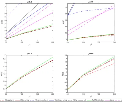
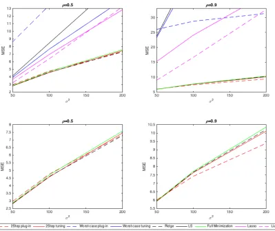
c∗ described in Section 2.2.3. Note that we tune all methods by BIC in the presented results. Simulation results for eachβare shown in Figure 2.1, 2.2, 2.3 and 2.4 respectively.
Results for β1, β2, and β3 are very similar. From the first row of each figure, it is clear
that OLS and worst-case estimators are the worst, while Lasso and Liu are better than
them sometimes but much worse than the other methods. Thus, we zoom in the results
for ridge estimator, full minimization method and two-step methods in the second row.
When ρ = 0.5, our two-step methods perform similarly to ridge estimator, while when
ρ = 0.9, the two-step with plug-in outperforms the other methods. However, under
either correlation, the full minimization method is not as good as expected. This may
be expected, as both β and σ2 require initial estimates, and either can be far from the
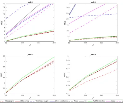
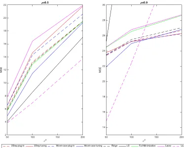
truth. Figure 2.4 shows the results for β4. When the true β comes from the worst-case
OLS estimator are better than the others. The ridge estimator is worse than both Liu’s
method, OLS and the worst-case with tuning method. However, whenρ= 0.9, OLS gets
much worse. Liu’s method is still the best with small variance, but it becomes unstable
when variance gets large. The worst-case with tuning method outperforms all the other
estimators except Liu’s estimator when variance is small, and is still stable when variance
becomes large. Note that when variance gets too large, all the estimators except OLS and
Liu’s method have similar performance and they all tend to shrink all the coefficients to
0.
In conclusion, our methods perform better when there is high correlation between
predictors, which is straightforward to check for real data sets. In general, the two-step
with plug-in method is similar to ridge estimator under low correlation, but outperforms
the others for high correlation, especially when the variance is large as well. In the
worst-case scenario, OLS and Liu’s method are better under low correlation, but they are much
worse than the worst-case controlling method under high correlation and large variance.
Thus, the worst-case method is a conservative choice for the worst-direction coefficients.
2.4
Pyrimidine Data
To illustrate our proposed methods, we apply them as well as the OLS, ridge, Lasso, and
Liu’s estimator to the Pyrimidine data (Hirst et al., 1994). This data set is used to study
the relationship between the structural properties and the activity of the inhibition of
dihydrofolate reductase (DHFR) by pyrimidines. It consists of 74 pyrimidines and their
structural information. The response is the logarithm of the inhibition constant assayed
from experiments. The predictors contain 26 attributes from 3 related positions, which
All predictors are centered and scaled to have mean 0 and variance 1. The response
variable is also centered before fitting. All estimators are tuned by BIC if necessary.
For our methods, we use either Ridge or Lasso estimator as the initial estimator. The
corresponding M matrix for ridge is simplyMridge = (XTX+λridgeIp)−1XT, while for
Lasso, MLasso = (XTX +λLassoW−)−1XT as described by Tibshirani (1996), where
W is a diagonal matrix whose jth diagonal is the absolute value of the jth element of
the Lasso estimate, and W− denotes the generalized inverse of W. We run 5-fold cross-validation using all the methods 100 times. Since the predictors in this data set are highly
correlated and of low variability, it is possible that the design matrix of some training
data sets appears to be rank deficient. Our two-step methods and full minimization
method do not have issues in such a situation based on Theorem 1 and equation (2.3)
as long as Xβ˜ 6= 0. The ridge and Lasso estimators can also handle rank deficiency. However, OLS, Liu’s method and the worst-case methods cannot be calculated uniquely
if X does not have full rank. The solution is setting the coefficients of the problematic
columns to be 0 before fitting. Similarly, sometimes althoughX is of rank p, XTX can be close to non-invertible so that the methods of OLS, Liu and the worst-case can be
unstable. The median of the 100 resulted mean squared prediction errors (MSPE) from
5-fold cross-validation is presented in Table 2.1, coupled with the estimated standard
deviation based on 1000 Bootstrap resamplings. The result is similar to the simulation.
The two-step methods can improve the performance of the initial estimator.
2.5
Discussion
In this chapter, we developed a class of linear estimators for linear regression which
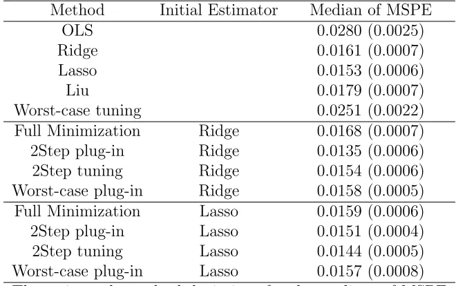
Table 2.1: Mean Squared Prediction Errors (MSPE) for the Pyrimidine Data
Method Initial Estimator Median of MSPE
OLS 0.0280 (0.0025)
Ridge 0.0161 (0.0007)
Lasso 0.0153 (0.0006)
Liu 0.0179 (0.0007)
Worst-case tuning 0.0251 (0.0022)
Full Minimization Ridge 0.0168 (0.0007)
2Step plug-in Ridge 0.0135 (0.0006)
2Step tuning Ridge 0.0154 (0.0006)
Worst-case plug-in Ridge 0.0158 (0.0005)
Full Minimization Lasso 0.0159 (0.0006)
2Step plug-in Lasso 0.0151 (0.0004)
2Step tuning Lasso 0.0144 (0.0005)
Worst-case plug-in Lasso 0.0157 (0.0008)
The estimated standard deviations for the medians of MSPE based on 1000 Bootstrap resamplings are showed in the paren-thesis.
and model variance are unknown, we proposed two methods. One is the full minimization
method, and the other is partial minimization. The former tries to minimize the mean
squared error as a whole, while the latter minimizes the variance for any given constraint
of bias. For the partial minimization approach, we further developed two ways to solve
it, the two-step method and the worst-case controlling method. The results of both the
simulation study and the real data example show that the two-step method can be the
best in general cases, while the worst-case controlling method can be the best choice for
Chapter 3
Testing and Estimation of Social
Network Dependence with Time to
Event Data
3.1
Introduction
With the development of internet, information propagates quickly along social network.
People can easily share information, such as ideas, pictures, articles or videos, to a lot of
friends through large social network platforms like Facebook, Twitter and QQ. In some
applications, it is interesting to find whether interaction between friends can affect the
propagation of events. For example, when people start playing an online game and send
invitations to their friends to join in, it is likely to see that some of their friends will
follow and start playing the same game. This is the case for Candy Crush, a very popular
game advertised through Facebook.
along network. Our study is motivated by data collected from players of a popular Tencent
QQ game. Due to the confidentiality, we are not allowed to disclose the name of the QQ
game. The network considered is the users’ friendship on Tencent QQ, which is a chatting
application widely used in China. Since friends can collaborate to win more experience
and tools, the game sends invitations to players’ friends asking them to join the game.
The times when users joined the game are recorded. Here, the time-to-event of interest is
defined as the time from the starting point, when the game was launched on Tencent QQ,
to the endpoint when a user joined to play the game. If a person never started playing the
game during the study period, the event time of this person is considered to be censored.
In addition, some demographic information of users, such as age and gender, is available.
Our goals here are to detect whether certain type of social network dependence exists
with time-to-event data and to quantify this dependence if it exists. In our considered QQ
game data application, an important feature for studying social network dependence is
that not all users will be influenced by friends. For example, for some users, whether they
will start playing the QQ game will not depend on their friends’ characteristics. Because
there is a cost on information targeting, it is of great interest to identify the subgroup of
people that are more likely to be influenced by their friends on a social network.
Towards these goals, we propose a latent Cox model with contextual effect. Our model
differs from the existing models in two aspects. First, the existing models are mainly for
uncensored data and most of them are based on linear regression models for responses.
Here, we incorporate the network dependence term in the conditional hazard function of
the event time to model the dependence between event times of connected users. Second,
a key difference is that most existing models (e.g. Zhu et al., 2017; Zhou et al., 2017)
assume the response of any user in the social network will be affected by his or her friends
indicator is introduced, indicating whether a user is susceptible to the influence of his or
her friends. Here, introducing the susceptible indicator not only increases the flexibility
for practical applications but also provides a way to estimate the probability that a user
might be affected by his or her friends’ characteristics in the social network. Therefore,
it can help to identify a subgroup of users who are more likely to be influenced by their
friends.
We first develop a score-type test for detecting the existence of the social network
dependence based on the proposed latent cox model with contextual effect. When the
social network dependence exists, we further develop an EM-type algorithm to estimate
the model parameters and derive the associated inference procedure. The remainder of
this chapter is organized as follows. In Section 3.2, we introduce the proposed model. In
Section 3.3, we present the proposed test statistic and estimation method. The asymptotic
properties of the proposed test and estimators are also established here. In Section 3.4,
simulations are conducted to evaluate the empirical performance of the proposed test and
estimators. An application of the proposed methods to analyze the time-to-event data
for playing the QQ game is given in Section 3.5, followed by discussions given in Section
3.6. All the technical derivations are provided in Appendix B.
3.2
Latent Cox Model with Contextual Effect
Let W = (Wij) ∈ {0,1}n×n be the adjacency matrix of a network involving n nodes,
where Wij = 1 means node iand node j are connected andWij = 0 otherwise. Let X =
(x1, . . . ,xn)T ∈Rn×p denote the covariate matrix which contains feature information of
n individuals in the network, such as age and gender of each person in the network. For
time. Define ˜Ti = min(Ti, Ci) and δi = I(Ti ≤ Ci). Our goal is to test and estimate
the dependence of event times among friends in the social network. A salient feature of
social network dependence is that not all the individuals are susceptible to their friends’
influence. To characterize the heterogeneity in susceptibility of individuals, we propose
the following latent Cox model with contextual effect for the conditional hazard function
for subject i:
λi(t|W,X, ξi) = λ(t)eβ
0x
i+ρξiPnj6=iWijβ0xj, (3.1)
where λ(t) is an unspecified baseline hazard function, β is a p-dimensional vector of
parameters andξi = 0/1 denotes the susceptibility indicator of individuali. In particular,
when ξi = 0, the event time of individual i does not depend on his or her friends’
characteristics. Moreover, we assume
P(ξi = 1|xi) =
eγ0x∗i
1 +eγ0x∗
i
, (3.2)
where x∗i = (1,x0i)0 and γ is a (p+ 1)-dimensional vector of parameters. Note that ρ is identifiable only when β does not equal to 0 and W is not a zero matrix. Throughout
this paper, we make these assumptions.
The parameter ρdescribes the magnitude of the dependence of a susceptible node to
its connected nodes, which is similar to the spatial autocorrelation parameter studied in
Zhou et al. (2017). When ρ = 0, there is no social network dependence between event
times of connected nodes. Under such a situation, the parameter γ is not estimable. In
the next section, we will first propose a test for the null hypothesis: H0 : ρ = 0, and
For convenience, it is assumed that Ci is independent of Ti. For example, in the QQ
game application, all the censoring times are equal to the total duration of the study.
This assumption is satisfied. However, this assumption can be relaxed as that Ci is
independent of Ti given covariates xi and those xj’s with Wij = 1. Our proposed test
and estimators are still valid.
3.3
Testing and Estimation Methods
3.3.1
Test for
H
0:
ρ
= 0
We propose a score-type tests statistic. Firstly suppose that ξ ≡ (ξ1, . . . , ξn)0 is known.
With the same argument as in Cox (1975), the partial likelihood function of the proposed
model (3.1) is
L(η;ξ) =
n Y
i=1
"
eβ0xi+ρξiPjn6=iWijβ0xj
Pn
l=1e
β0x
l+ρξlPnj6=lWljβ0xjI( ˜T
l ≥T˜i)
#δi
, (3.3)
where η = (ρ,β0)0. Under H0, model (3.1) becomes the standard Cox proportional haz-ards model. Let ˜βdenote the maximum partial likelihood estimator under the null. Define
˜
η= (0,β˜0)0. Then, the score statistic is given by
S1( ˜η;ξ) =
∂log(L)
∂ρ
η=η˜
=
n X
i=1
δi (
ˆ
Zi − Pn
l=1e
˜
β0xlI( ˜T
l≥t˜i) ˆZl
Pn
l=1e
˜
β0x
lI( ˜T
l ≥˜ti)
)
=
n X
i=1
Z τ
0
(
ˆ
Zi− Pn
l=1e
˜
β0xlI( ˜T
l ≥s) ˆZl
Pn
l=1e
˜
β0x
lI( ˜T
l ≥s)
)
where τ is the total study duration, ˆZi =ξiPnj6=iWijβ˜
0x
j and
ˆ
Mi(s) = Ni(s)−
Z s
0
eβ˜0xiI( ˜T
i ≥u)dΛ(˜ u),
with Ni(s) = δiI( ˜Ti ≤ s) and ˜Λ(u) =
Ru
0
Pn i=1dNi(t)
Pn
j=1I( ˜Tj≥t)e
˜
β0xj being the Breslow estimator of the baseline cumulative hazard function under the null.
Since ξ is unknown in practice, we replace ξi with its expectation pi ≡P(ξi = 1|xi)
given in (3.2). Specifically, define ˆZi∗ = piPnj6=iWijβ˜
0x
j. By replacing ˆZi with ˆZi∗ in
equation (3.4), we obtain a new score-type statistic, denoted byS1∗( ˜η;γ). Note thatγ is not identifiable under the null. Following the similar technique used in Fan et al. (2016)
for testing the existence of a subgroup with an enhanced treatment effect, we propose
the following supremum score test statistic:
Tn = sup
γ∈Γ
{S1∗( ˜η;γ)}2
Pn
i=1
n
ψi∗( ˜η,Λ;˜ γ)o 2.
Here, Γ is the domain of γ, which is usually Rp+1. In practice, the supreme is obtained by a grid search over Γ. ψi∗( ˜η,Λ;˜ γ) in the denominator is defined as
ψ∗i( ˜η,Λ;˜ γ) =
Z τ
0
"
ˆ
Zi∗−
Pn
l=1e
˜
β0xlI( ˜T
l≥s) ˆZl∗
Pn
l=1e
˜
β0x
lI( ˜T
l≥s)
−
I∗12,n( ˜η)I−1 22,n( ˜η)
(
xi− Pn
l=1e
˜
β0xlI( ˜T
l≥s)xl
Pn
l=1e
˜
β0x
lI( ˜T
l ≥s)
)#
dMˆi(s),
where I22,n( ˜η) =−∂
2log(L)
∂ββ0 |η= ˜η, I12,n( ˜η) =−∂
2log(L)
∂ρ∂β0 |η= ˜η, and I∗12,n( ˜η) is obtained from
In the Appendix, we show that under the null,
1 √
nS
∗
1( ˜η;γ) = 1 √
n
n X
i=1
ψ∗i( ˜η0,Λ˜0;γ) +op(1),
where ˜η0 = (0,β˜00)
0 and ψ∗
i( ˜η0,Λ˜0;γ) can be obtained from ψ∗i( ˜η,Λ;˜ γ) by replacing ˜β
with ˜β0 and ˜Λ with ˜Λ0. Here, ˜β0 and ˜Λ0 are the true values of β and Λ, respectively,
under the null. By applying the martingale central limit theorem, we haven−1/2S∗
1( ˜η;γ) converges in distribution to a mean-zero normal variable under the null, with the
asymp-totic variance being consistently estimated byn−1Pni=1{ψi∗( ˜η,Λ;˜ γ)}2. Therefore, we can establish the asymptotic null distribution of the test statisticTn in the following theorem.
Theorem 3. Under mild regularity conditions,Tn converges in distribution tosup
γ∈Γ
G2(γ)
under H0 as n → ∞, where {G(γ) : γ ∈ Γ} is a mean zero Gaussian process with the
covariance function
Σ(γ1,γ2) = lim
n→∞
Pn
i=1ψ
∗
i( ˜η0,Λ˜0;γ1)ψ∗i( ˜η0,Λ˜0;γ2)
q Pn
i=1{ψ
∗
i( ˜η,Λ;˜ γ1)}2
Pn
i=1{ψ
∗
i( ˜η,Λ;˜ γ2)}2
,
for any γ1,γ2 ∈Γ.
The proof of Theorem 3 is given in Appendix B.1. To obtain the critical value of
the asymptotic null distribution of Tn, we adopt a resampling method. Specifically, we
consider the perturbed test statistic
Tn∗ = sup
γ∈Γ
n Pn
i=1φiψ
∗
i( ˜η,Λ;˜ γ)
o2
Pn
i=1
n
ψ∗
i( ˜η,Λ;˜ γ)
o2 ,
have the same asymptotic null distribution. Therefore, we can generate a large number
of perturbed statistics and use the empirical upper α-quantile of the perturbed statistics
to estimate the critical value Cα for an α-level test. The null hypothesis is rejected if
Tn > Cα.
3.3.2
Parameter Estimation
Throughout this section, we assume ρ 6= 0. Under such an assumption, the parameters
in models (3.1) and (3.2) are identifiable. We develop an EM-type algorithm to estimate
the model parameters, denoted by Θ= (β0, ρ,γ0)0 and Λ(t) =R0tλ(u)du. Define Λi(t) =
eβ0xi+ρξiPnj6=iWijβ0xjΛ(t). The complete log likelihood function is
l(Θ,Λ) =
n X
i=1
"
δi{logλ( ˜Ti) +β0xi+ρξi n X
j6=i
Wijβ0xj} −Λi( ˜Ti) +ξiγ0x∗i −log(1 +e
γ0x∗
i)
#
.
(3.5)
Let ˆΘ(k)and ˆΛ(k) denote the estimators ofΘand Λ at thekth iteration, respectively, and
Ωdenote the observed data,{( ˜Ti, δi,xi) :i= 1, . . . , n}andW. At the (k+1)th iteration,
in the E-step, we calculate the conditional expectation of l(Θ,Λ) given observed dataΩ
and current estimators ˆΘ(k) and ˆΛ(k) of the parameters. Specifically,
Q(Θ,Λ|Θˆ(k),Λˆ(k))≡E{l(Θ,Λ)|Ω,Θˆ(k),Λˆ(k)} =
n X
i=1
"
δi{logλ( ˜Ti) +β0xi+ρA
(k)
i n X
j6=i
Wijβ0xj} −B
(k)
i +A
(k)
i γ
0
x∗i −log(1 +eγ0x∗i)
#
,
where
A(ik) = E(ξi|Ω,Θˆ(k),Λˆ(k))
= e
δiρˆ(k)Pnj6=iWijβˆ(k)0xje−e
ˆ
β(k)0xi+ ˆρ(k)Pn
j6=iWijβˆ(k)
0x
jΛˆ(k)( ˜T
i)pˆ(k)
i
eδiρˆ(k)Pnj6=iWijβˆ(k)0xje−eβˆ
(k)0x
i+ ˆρ(k)Pnj6=iWijβˆ(k)
0x
jΛˆ(k)( ˜T
i)pˆ(k)
i +e−e
ˆ
β(k)0xiΛˆ(k)( ˜T
i)(1−pˆ(k)
i )
,
Bi(k) =E{Λi( ˜Ti)|Ω,Θˆ(k),Λˆ(k)}= (1−A
(k)
i )e
β0xiΛ( ˜T
i) +A
(k)
i e
β0xi+ρ
Pn
j6=iWijβ0xjΛ( ˜T
i),
and ˆp(ik)= exp(ˆγ(k)0x∗i)/{1 + exp(ˆγ(k)0x∗i)}.
The function Q(Θ,Λ|Θˆ(k),Λˆ(k)) can be written as the summation of l1(β, ρ,Λ) and l2(γ), where
l1(β, ρ,Λ) =
n X
i=1
h
δi{logλ( ˜Ti) +β0xi+ρA
(k)
i n X
j6=i
Wijβ0xj}
−eβ0xiΛ( ˜T
i){(1−A
(k)
i ) +A
(k)
i e
ρPn
j6=iWijβ0xj}
i
,
l2(γ) =
n X
i=1
n
A(ik)γ0xi∗−log(1 +eγ0x∗i)
o
.
In the M-step, we maximize the functions l1(β, ρ,Λ) and l2(γ) separately. Note that
l2(γ) has a form similar to the log likelihood function for a logistic regression. It can be
maximized directly using many existing gradient-based methods. Let ˆγ(k+1) denote the
resulting maximizer. The function l1(β, ρ,Λ) involves the nonparametric function Λ. To
maximizel1(β, ρ,Λ), a log profile likelihood is first constructed. Similar to the arguments in Johansen (1983) and Klein (1992), whenβandρare fixed, the nonparametric estimator
that maximizesl1(β, ρ,Λ) is given by
ˆ
Λ(k+1)(t;β, ρ) =
n X
i=1
Z t
0
dNi(s) Pn
j=1I( ˜Tj ≥s)eβ
0x
j{(1−A(k)
j ) +A
(k)
j e
ρPn
l6=jWjlβ0xl}
Plugging ˆΛ(k+1)(t;β, ρ) intol
1(β, ρ,Λ), the log profile likelihood function forβ andρ, up to some constant, is
pl1(β, ρ) =
n X
i=1
δi β0xi+ρA
(k)
i n X
j6=i
Wijβ0xj
−log
" n
X
j=1
I( ˜Tj ≥T˜i)eβ
0x
j
n
(1−A(jk)) +A(jk)eρPnl6=jWjlβ0xl
o #!
.
The log profile likelihood function pl1(β, ρ) is not concave in β and ρ. To maximize it,
we propose an iterative optimization method. Specifically, given β, pl1(β, ρ) is a
uni-variate concave function of ρ, so it can be easily maximized with respect to ρ. Let
ˆ
ρ(k+1) = arg max
ρ
pl1( ˆβ(k), ρ). Updating β given ρ is not straightforward. To facilitate the optimization with the computational stability, we fix ρ = ˆρ(k+1) and β = ˆβ(k) in
the terms ρA(ik)Pnj=6 iWijβ0xj and A
(k)
j e
ρPn
l6=jWjlβ0xl of pl
1(β, ρ). Then, the log profile likelihood function pl1(β, ρ) can be written as, up to some constant,
n X
i=1
δi β0xi−log
" n
X
j=1
I( ˜Tj ≥T˜i)eβ
0x
j
n
(1−A(jk)) +A(jk)eρˆ(k+1)Pnl6=jWjlβˆ(k)0xl
o #!
,
which is equivalent to fit a Cox model with regression parametersβand an offset log{(1−
A(jk)) +A(jk)eρˆ(k+1)Pnl6=jWjlβˆ(k)0xl} for the jth subject, j = 1, . . . , n. Let ˆβ(k+1) denote the
maximizer of the above function. Define ˆΛ(k+1)(t) = ˆΛ(k+1)(t; ˆβ(k+1),ρˆ(k+1)). We iterate
the E-step and M-step until convergence. Let ˆΘ and ˆΛ denote the resulting estimators of Θand Λ, respectively, at convergence. Ideally, at each iteration of the EM algorithm,
ρ and β should be updated iteratively till convergence. However, to make the algorithm
faster and stable, we just updateρandβonce in each EM iteration. When the algorithm
In our EM algorithm, we chose the initial estimators of the parameters as follows: ˆρ(0) = 0,
ˆ
γ(0) = 0, ˆβ(0) is the maximum partial likelihood estimator and ˆΛ(0) is the Breslow’s estimator under the standard Cox model whenρ= 0. In addition, the convergence criteria
was set as ||Θˆ(k+1)−Θˆ(k)||
∞ < 10−6. Based on our numerical experience, the proposed
EM algorithm usually converges within 50 iterations. It is worth noting that the term
A(ik) at convergence denotes the posterior probability that the ith user might be affected
by his or her friends’ behavior. We name it the posterior “susceptible” probability.
Let Θ0 and Λ0 denote the true values of Θ and Λ, respectively. The asymptotic properties of the proposed estimators are established in the following theorem.
Theorem 4. Under mild regularity conditions, we have, as n → ∞,
sup
t∈[0,τ]
|Λ(ˆ t)−Λ0(t)| →0 and ||Θˆ −Θ0|| →0 a.s.
In addition, √n{Θˆ −Θ0} converges in distribution to a mean-zero multivariate normal
variable.
The proof of Theorem 4 is given in Appendix B.2. Next, we derive a method for
esti-mating the asymptotic variance of ˆΘ. We adopt the techniques developed in Lange (1999) and Hunter and Lange (2004) for estimating the variance of MM estimators. Specifically,
define g(Θ|Θˆ(k)) = pl
1(β, ρ) +l2(γ). Let ∇2g(Θ|Θˆ(k)) denote the second derivative of g(Θ|Θˆ(k)) with respect to Θ. Note that ∇2g(Θ|Θˆ(k)) has explicit expressions, which are provided in Appendix B.3. Then, the observed information matrix can be approximated
by
I( ˆΘ) = −∇2g( ˆΘ|Θˆ)
n
I− ∇M( ˆΘ)
o
where M(ν) = arg maxΘ g(Θ|ν) and ∇M(ν) = ∂M(ν)/∂ν0. The inverse of I( ˆΘ) is an estimator of the asymptotic covariance matrix of ˆΘ. Here, ∇M(ν) does not have an explicit expression and we compute it by numerical differentiation. Specifically, write
M( ˆΘ) = {M1( ˆΘ), . . . , Mq( ˆΘ)}0, where q = 2(p+ 1). The (i, j)th element of ∇M( ˆΘ) is
computed by {Mi( ˆΘ+dej)−Mi( ˆΘ)}/d, where d is a small positive value and ej is the
basis vector with thejth element as 1 and others as 0. Note that when the EM algorithm
converges, M( ˆΘ) = ˆΘ. To compute M( ˆΘ+dej), we fix ν = ˆΘ+dej and compute the
maximizer ofg(Θ|ν) using the proposed EM algorithm. In our implementation, we chose
d=d0/n, whered0 is a small positive constant. We have tried a few values ofd0, ranging
from 1 to 10, and found that d0 = 5 gives reasonable variance estimates for all cases.
3.4
Simulation Studies
In this section, we conduct simulations to evaluate the empirical performance of the
proposed test and estimators. The underlying network is generated from the stochastic
block model (Holland et al., 1983). LetK be the number of communities in the network.
The stochastic block model is defined by
P(Wij = 1) = 1−P(Wij = 0) =PCiCj, (3.9)
whereP is aK×K symmetric matrix whose (Ci, Cj)th elementPCiCj records the
prob-ability that communitiesCi andCj are connected. The total number of nodesn is set to
be 2000 andK is set to be 1, 5 or 10. ForK = 5, the numbers of nodes contained in each
community are (500,500,400,400,200) and the corresponding P matrix has elements
P11 =P33 = 0.05, P22 =P55 = 0.1, P44 = 0.2 and PCiCj = 10
−4 for C
when K = 10, community sizes are (100,100,100,100,200,200,200,200,400,400) and
P11 = P55 = 0.05, P22 =P66 = P99 = P10,10 = 0.1, P33 = P77 = 0.2, P44 = P88 = 0.3
and PCiCj = 10
−4 if C
i 6= Cj. For K = 1, we generate the network from a pseudo
5-community stochastic block model with 5-community numbers same as in K = 5, and
P11 = P22 =P33 =P44 = 0.01, P55 = 0.3, PCiCj = 0.015 for Ci 6=Cj. All communities
are quite connected without clear separation, while a subset of nodes are connected more
closely. Such network structure is similar to the observation in the real data example.
The baseline hazard function is chosen as λ0(t) = 0.5. Two covariates are included,
where the first covariate is generated from a Bernoulli distribution with the success
probability 0.5 and the second is generate from a uniform distribution on (-1, 1). We
set β = (1,−1)0 and γ = (0,1,−1)0. The censoring time is generated from a uniform distribution on (0, c), where the constant c is chosen to yield the approximately 15% or
30% censoring rate. We conduct 1000 replicates for each simulation setting.
3.4.1
Simulation Results for Testing
We consider the following values of ρ: 0, 0.01, 0.015, 0.02 and 0.05, and conduct the
proposed test with the alpha-level as 0.05. When computing the p-value of the test
statistic, we generate 1000 perturbed test statistics as described in Section 3.3.1. The
empirical type I error and power of the proposed test are reported in Table 3.1. It can be
seen that the proposed test gives proper type I error rates under the null whenρ= 0. In
addition, the power of the test increases as ρ increases and the censoring rate decreases