ABSTRACT
KIM, SEONG-TAE. A New Approach to Unit Root Tests in Univariate Time Series Robust to Structural Changes. (Under the direction of Dr. David A. Dickey.)
Using methodology in panel unit root tests we propose a new approach to uni-variate unit root tests. Our method leads to an asymptotically normal distribution of the least squares estimator and is robust to contaminated data having structural changes or outliers while the power of the test does not drastically worsen.
The main idea is that under the assumption that the process has a unit root we transform an AR(1) process {yt : 1 ≤ t ≤ T} to a double-index process {yij : 1 ≤ i ≤ m,1 ≤ j ≤ n, mn = T} in such a way that the segments are independent for
i= 1,2,· · · , m. For this transformed data, we apply the same sequential limit as in Levin and Lin (1992, 2002). First, as n → ∞ we obtain asymptotic results for each
A New Approach to Unit Root Tests in Univariate Time Series Robust to Structural Changes
by
Seong-Tae Kim
A dissertation submitted to the Graduate Faculty of North Carolina State University
in partial fulfillment of the requirements for the Degree of
Doctor of Philosophy
STATISTICS
Raleigh 2006
APPROVED BY:
Professor David A. Dickey Professor Bibhuti B. Bhattacharyya Chair of Advisory Committee
To my dad,
Jeong-Cheol Kim,
who I regret will never be able to share my happiness at my great
moment in person
Biography
Acknowledgements
I would like to express my deepest gratitude and biggest appreciation to the people supported to complete this dissertation. First of all, my deepest appreciation goes out to my advisor Dr. David A. Dickey for his guidance, patience, and encouragement during my research. I also appreciate my committee members Dr. Sastry G. Pantula, Dr. Bibhuti B. Bhattacharyya and Dr. Alastair R. Hall. They not only provided me with valuable information and instruction through my research but also gave me a chance to upgrade my knowledge through their impressive classes.
I must acknowledge as well my friends, colleagues, and faculty members. I will never forget the moment of Dr. William Swallow visiting the ER at Rex Hospital when I passed out. It goes without saying that his sudden visiting deeply touched my heart. I wholeheartedly thank my friends, Man Sik Park and Jung Wook Park and their family. They have been the greatest supporter for my studies as well as they have shared my joy and sorrow.
Contents
List of Tables vii
List of Figures viii
1 Introduction 1
1.1 Statement of the Problem . . . 1
1.2 Literature Review . . . 4
1.2.1 Asymptotic normality in unit root tests . . . 4
1.2.2 Panel Unit Root Tests . . . 8
1.2.3 Structural change . . . 13
1.3 Summary of chapters . . . 15
2 Data Transformation and Asymptotics 18 2.1 Multi-index transformation of random variables . . . 19
2.2 Growth rate of m and n . . . 24
3 Estimation 30 3.1 Model I: Simple AR (1) model . . . 33
3.1.1 Model setup . . . 33
3.1.2 Estimation and asymptotic results . . . 36
3.1.3 Behavior under the alternative . . . 40
3.2 Model 2: Intercept AR (1) model . . . 46
3.2.1 Global mean model: M2-G . . . 48
3.2.2 Interval-specific mean model . . . 51
3.3 Model III: Linear trend AR (1) model . . . 59
3.3.1 Global parameter model: M3-G and M3-GD . . . 60
3.3.2 Interval-specific parameter model: M3-I and M3-ID . . . 64
3.4 Simulation Results . . . 69
4 Data Contamination and Unit Root Tests 83
4.1 Data contamination . . . 83
4.2 Asymptotic Behavior . . . 91
4.3 Spurious rejection with structural change and size distortion . . . 95
4.4 Finite sample behavior in the presence of structural change . . . 100
5 Empirical Data Analysis 107 5.1 A small sample case: US GDP data . . . 108
5.2 A large sample case: US/Canada daily exchange rate . . . 117
6 Conclusion 121 6.1 Findings . . . 121
6.2 Future Studies . . . 122
Bibliography 123 7 Appendices 131 7.1 Critical Values and Power of Basic Models . . . 131
7.2 Histogram of Statistics . . . 142
7.3 Empirical Power of Basic Models . . . 148
7.4 Empirical Power in the Presence of Single Break . . . 155
List of Tables
2.1 Independent Transformation . . . 23
3.1 Data Transformation Process . . . 34
3.2 Moments of an Simple AR(1) Model (Dickey, 1976) . . . 39
3.3 Moments of the Intercept AR(1) Model (Dickey, 1976) . . . 54
3.4 Moments of the Linear Trend AR (1) Model (Dickey, 1976) . . . 67
3.5 Simulation scheme: Selection of m and n fromT . . . 70
4.1 Power Comparison of DF, Perron, and KD Approach . . . 105
5.1 Unit Root Tests for Annual US Real GDP: M3-G . . . 110
5.2 Unit Root Tests for Annual US Real GDP: M3-I . . . 111
5.3 Unit Root Tests for Quarterly US Real GDP: M3-G . . . 114
5.4 Unit Root Tests for Quarterly US Real GDP: M3-I . . . 115
5.5 Variation inn with fixedm: M3-G . . . 116
5.6 Unit Root Tests for US/Canada Exchange Rate . . . 119
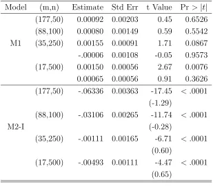
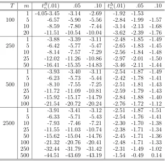
7.1 Critical values ofρ and t-statistics in M1 . . . 132
7.2 Critical values ofρµ and tµ-statistics in M2-G . . . 133
7.3 Critical values oftµi and t BC µi -statistics in M2-I . . . 134
7.4 Critical values ofρτ and tτ-statistics in M3-G . . . 135
7.5 Critical values oftτi and t BC τi -statistics in M3-I . . . 136
7.6 Empirical Power oft-statistic in M1 . . . 137
7.7 Empirical Power oft-statistic in M2-G . . . 138
7.8 Empirical Power oft-statistic in M3-G . . . 139
7.9 Empirical Power oft-statistic in M2-I . . . 140
List of Figures
3.1 Transformation of Simple AR (1) Model . . . 35
3.2 Transformation of Intercept AR (1) Model . . . 47
3.3 Transformation of Linear Trend AR (1) Model:M3-G . . . 60
3.4 Transformation of Linear Trend AR (1) Model: M3-I . . . 66
4.1 Transformation of M2-G with Structural Change . . . 86
4.2 Transformation of M3 with Trend Shift . . . 87
4.3 Slope Change in Model 3 . . . 89
4.4 Trend Shift and Slope Change in Model 3 . . . 90
4.5 Empirical Size of t(0.05) with Break in Level in M2-G [T=100, m=5] 98 4.6 Actual Size of t(0.05) with Break in Level in M2-G [T=100, m=5] . . 99
5.1 The Log Valued Annual US Real GDP: 1870-1994 . . . 109
5.2 Transformation of Annual US GDP: m = 6, n = 20 . . . 110
5.3 The Log Valued Quarterly US Real GDP: 1947:1-2006:4 . . . 114
5.4 Transformation of Quarterly US GDP: m = 6, n = 40 . . . 115
5.5 Nominal US/Canada Exchange Rate: 1/4/1971-5/19/2006 . . . 117
5.6 Transformation (a) of US/Canada Exchange Rate: m = 35, n = 250 . 118 5.7 Transformation (b) of US/Canada Exchange Rate: m = 35, n = 250 . 118 7.1 Density of t-statistic in M1 (T=100) . . . 142
7.2 Density of t-statistic in M1 (T=250) . . . 143
7.3 Density of t-statistic in M2-G (T=100) . . . 144
7.4 Density of t-statistic in M3-G (T=100) . . . 145
7.5 Density of t-statistic in M2-I (T=100) . . . 146
7.6 Density of t-statistic in M3-I (T=100) . . . 147
7.7 Empirical Power of t-statistic in M1 . . . 148
7.8 Empirical Power oft−statistic in M2-G . . . 149
7.9 Empirical Power oft−statistic in M3-G . . . 150
7.10 Empirical Power of tbiased in M2-I . . . 151
7.11 Empirical Power of tbc in M2-I . . . 152
7.13 Empirical Power of tbc in M3-I . . . 154
7.14 Empirical Power of t(0.05)[T = 100, ρ= 0.9, α1 = 2.5] . . . 155
7.15 Empirical Power of t(0.05)[T = 100, ρ= 0.9, α1 = 5] . . . 156
7.16 Empirical Power of t(0.05)[T = 100, ρ= 0.9, α1 = 10] . . . 156
7.17 Empirical Power of tµ(0.05)[T = 100, ρ= 0.9, α1 = 2.5] . . . 157
7.18 Empirical Power of tµ(0.05)[T = 100, ρ= 0.9, α1 = 5] . . . 157
7.19 Empirical Power of tµ(0.05)[T = 100, ρ= 0.9, α1 = 10] . . . 158
7.20 Size-Adjusted Empirical Power of tµ(0.05)[T = 100, ρ= 0.9, α1 = 2.5] 158 7.21 Size-Adjusted Empirical Power of tµ(0.05)[T = 100, ρ= 0.9, α1 = 5] . 159 7.22 Size-Adjusted Empirical Power of tµ(0.05)[T = 100, ρ= 0.9, α1 = 10] . 159 7.23 Empirical Power of tµi(0.05)[T = 100, ρ= 0.9, α1 = 2.5] . . . 160
7.24 Empirical Power of tµi(0.05)[T = 100, ρ= 0.9, α1 = 5] . . . 160
7.25 Empirical Power of tµi(0.05)[T = 100, ρ= 0.9, α1 = 10] . . . 161
7.26 Empirical Power of tτ(0.05)[T = 100, ρ= 0.9, α1 = 2.5] . . . 162
7.27 Empirical Power of tτ(0.05)[T = 100, ρ= 0.9, α1 = 5] . . . 162
7.28 Empirical Power of tτ(0.05)[T = 100, ρ= 0.9, α1 = 10] . . . 163
7.29 Size-Adjusted Empirical Power of tτ(0.05)[T = 100, ρ= 0.9, α1 = 2.5] 163 7.30 Size-Adjusted Empirical Power of tτ(0.05)[T = 100, ρ= 0.9, α1 = 5] . 164 7.31 Size-Adjusted Empirical Power of tτ(0.05)[T = 100, ρ= 0.9, α1 = 10] . 164 7.32 Empirical Power of tτ(0.05)[T = 100, ρ= 0.90, α1 = 2.5] . . . 165
7.33 Empirical Power of tτ(0.05)[T = 100, ρ= 0.90, α1 = 5] . . . 165
7.34 Empirical Power of tτ(0.05)[T = 100, ρ= 0.90, α1 = 10] . . . 166
7.35 Empirical Power of tτ(0.05)[T = 100, ρ= 0.9, β1 = 1, β2 =.2] . . . 167
7.36 Size Adjusted Power of tτ(0.05)[T = 100, ρ= 0.9, β1 = 1, β2 =.2] . . . 167
7.37 Empirical Power of tτ(0.05)[T = 100, ρ= 0.9, β1 = 1, β2 =.5] . . . 168
7.38 Size Adjusted Power of tτ(0.05)[T = 100, ρ= 0.9, β1 = 1, β2 =.5] . . . 168
7.39 Empirical Power of tτi(0.05)[T = 100, ρ= 0.9, β1 = 1, β2 =.2] . . . 169
7.40 Size Adjusted Power of tτi(0.05)[T = 100, ρ= 0.9, β1 = 1, β2 =.2] . . 169
7.41 Empirical Power of tτi(0.05)[T = 100, ρ= 0.9, β1 = 1, β2 =.5] . . . 170
7.42 Size Adjusted Power of tτi(0.05)[T = 100, ρ= 0.9, β1 = 1, β2 =.5] . . 170
7.43 Empirical Power of tµ(0.05)[T = 100, ρ= 0.9, α1 = 2.5, α2 = 2.5] . . . 171
7.44 Size Adjusted Power of tµ(0.05)[T = 100, ρ= 0.9, α1 = 2.5, α2 = 2.5] . 171 7.45 Empirical Power of tµ(0.05)[T = 100, ρ= 0.9, α1 = 2.5, α2 =−5] . . . 172
Chapter 1
Introduction
1.1
Statement of the Problem
It is well known that the limiting distributions of standard unit root tests are non-normal. These distributions are called “Dickey-Fuller distributions.” Under the null hypothesis of a unit root, the limiting distributions are usually represented by functionals of standard Brownian motion. Although the asymptotic non-normality is not as serious as low testing power and sensitivity to model specification, it is inconvenient to use nonstandard tables as in Dickey (1976) or Fuller (1996). Hence, our research focuses on robustness to structural change and asymptotic normality. In this paper, we obtain the asymptotic normality in univariate unit root tests under local detrending using the methodology in panel unit root tests. Our approach is robust under the situation where there are structural changes or outliers while the power of the test does not drastically worsen.
The estimation models usually considered in standard unit root tests are:
Model 1: Yt=ρYt−1 +ǫt (1.1)
Model 2: Yt=µ+ρYt−1+ǫt (1.2)
Model 3: Yt=α+βt+ρYt−1+ǫt (1.3)
The corresponding estimators and their asymptotics are: Model 1: ρˆ=
Pn
t=2YtYt−1
Pn t=2Yt2−1
n(ˆρ−1) ⇒
1 2{W
2(1)−1}
R1
0 W2(r)dr
and ˆt ⇒
1 2{W
2(1)−1}
R1
0 W2(r)dr
1/2
Model 2: ρˆµ= Pn
t=2P(Yt−y¯(0))(Yt−1−y¯(−1)) n
t=2(Yt−1−y¯(−1))2
n(ˆρµ−1) ⇒ R1
0RΨ(r)dW
Ψ2dr and ˆtµ ⇒
R1
0 Ψ(r)dW
R
where Ψ =W(r)−R W(r)dr.
Model 3: ρˆτ = PT
t=2yˆtyˆt−1
PT t=2yˆt2−1
, yˆt =yt−αˆ−βtˆ
n(ˆρτ −1) ⇒ R
W(r)dW +N
D and ˆtτ ⇒
R
W(r)dW +N D1/2
where
N = 12
Z
rW(r)dr−1
2
Z
W(r)dr Z
W(r)dr− 1
2W(1)
−W(1)
Z
W(r)dr
D=
Z
W2(r)dr−12
Z
rW(r)dr 2
+12
Z
W(r)dr Z
rW(r)dr−4
Z
W(r)dr 2
.
Researchers have studied structural change in the variance of the error process and structural changes in the parameters, µ, α, and β in Model 2 and Model 3. In the unit root test, the structural change leads to a different estimator of ρ and different asymptotic behavior where the estimator and limiting distribution depend on the break point and/or break size.
The main idea of the paper is that under the assumption that the process has a unit root we transform a univariate time series process {Yt : 1 ≤ t ≤ T} to a
double-index process {yij : 1 ≤ i ≤ m,1 ≤ j ≤ n, mn = T} in such a way that the
technique is that an undetected break has a relatively minor effect on the asymptotic results which, in fact, disappears as m increases.
1.2
Literature Review
Literature review concentrates on three topics. They are unit root tests in panel data, univariate unit root tests with asymptotic normality, and unit root tests with structural changes since we adopt the methodology of panel unit root tests to achieve asymptotic normality, especially, under the situation of structural change. See Mad-dala and Kim (1998) and references therein for various issues in unit root tests.
1.2.1
Asymptotic normality in unit root tests
Lai and Siegmund (1983)
Lai and Siegmund (1983) showed that for a simple non-explosive AR (1) model if data follow a particular stopping rule, the OLS estimator of ρ is asymptotically normally distributed uniformly in ρ. Consider the simple non-explosive AR(1) model with unknown parameter ρ∈[−1,1]
yt=ρyt−1 + ǫt, t= 1,2,· · ·
whereǫt arei.i.d.with Eǫ1 = 0 and Eǫ21 =σ2. For c >0 let the optimal stopping rule
be
Tc = inf{t: t X
i=1
Then uniformly in ρ and t ∈(−∞,∞),
Pρ
c−1/2 Tc X
i=1
yi−1ǫi ≤t
→Φ(t) as c→ ∞. (1.5)
Now define
Nc = first n≥1 such that In≥cσ2. (1.6)
Then for the OLS estimator of ρ,
IN1/c2(ρc−ρ) d
−→N(0, σ2) uniformly in ρ∈[−1,1] (1.7)
where In =−d
2
dρ2
ρPni=1yi−1yi− 12ρ2Pni=1y2i−1
=Pni=1y2
i−1, which is the observed
Fisher information about ρ.
Although this approach has the nice asymptotic normality, it has two main draw-backs: (1) it is hard to extend to a complicated model,i.e., linear trend model. Re-cently, Chang and Park (2004) extended the results to the local-to-unity hypothesis and AR(1) model with intercept; (2) According to the optimal stopping rule in their paper, the choice of c is totally arbitrary. This means that the value of c must be chosen a priori regardless of the pattern of a data set.
Breitung and Hassler (2002)
Breitung and Hassler (2002) proposed an asymptotically normally distributedt−statistic for H0 : zt ∼ I(1) against H1 : zt is fractionally integrated. Letting yt = ∆zt = zt−zt−1, the estimation regression is given by
yt=ρyt∗−1+ǫt,
whereyt∗−1 =
Pt−1 j=1
yt−j j =
Pt−1 j=1
∆zt−j
j and ǫt are i.i.d.with E(ǫt) = 0 and E(ǫ 2
t) =σ2.
results as T → ∞
tρ−→d N(0, 1) T ·R2 −→d χ2(1)
where R2 is the coefficient of determination. Although this approach achieves the
asymptotic normality, the alternative is different from our framework.
Phillips, Moon, Xiao (2001)
Phillips et al. suggested a method of blocking a univariate time series to estimate the local to unity parameter. They first consider the following AR(1) model with the local to unity parameter:
yt =ayt−1+ut, a= 1 + c
n, ut ∼ iid(0, σ
2), t = 1,2,
· · · , n, c < 0.
The block local to unity model they proposed is defined as follows:
yk,t = ayk,t−1+uk,t, t={1,· · · , m}; k = 1,· · · , M, yk,0 = yk−1,m,
a = ec/m∼1 + c m.
(1.8)
In this transformation, the total number of observations,n, is divided intoM blocks of m observations. Another feature is that the initial value of each interval is the last value of the previous interval. Using this transformation, they found the limiting distributions of ˆa depending on the local to unity parameterc.
(1) c <0 : √M m(ˆa−a)⇒N(0,−2c) (2) c= 0 : M m(ˆa−a)⇒
Z
W2(r)dr−1 Z
W(r)dW.
the case of c < 0, they still had the same limiting distribution as the Dickey-Fuller test for the unit root case. We reference this method since our method also uses the blocking method in (1.8).
Kunst (1997)
The circular χ2 family in Kunst (1997) is another double-index transformation of a
univariate time series. Kunst focused on the univariate process {Yt} expressed as
(Y1,Y2,· · · , Yn, Yn+1,· · ·) = (X1,1, X2,1,· · · , Xn,1, X1,2,· · ·)
or equivalently, with [x] for the integer part of x,
Yt=Xt−n[(t−1)/n],[(t−1)/n]+1, t= 1,· · · , T;
where n is an arbitrary finite integer, and (X1,t,· · · , Xn,t) is a finite sequence of n
mutually independent random walks. This kind of transformation is quite similar to the seasonality model although the value ofnis not restricted to the specific seasonal values such as n = 2,4,12. However, since n does not grow the asymptotic results are affected only by T. The circular χ2 distribution with periodicityn is given by:
βn(T) = ˆσ−2hn(T)′Hn(T)−1hn(T)
where
Hn(T) = (Hij(T))i,j=1,···,n =
XT
t=max(i,j)+1
Yt−iYt−j
/T2
and with ∆nYt =Yt−Yt−n,
hn(T) =
T−1 T X
t=2
Yt−1∆nYt,· · · , T−1 T X
t=n+1
Yt−n∆nYt ′
To obtain the asymptotic result for βn(T), he proved the following results:
T−2 T X
t=j+1
Yt−iYt−j ⇒σ2n−1 n X
l=1
Z 1
0
Wl(r)Wl+j−i−n[(l+j−i−1)/n](r)dr,
T−2 T X
t=1
Yt2 ⇒σ2n−1 n X
l=1
Z 1
0
Wl2(r)dr,
and
T−1 T X
t=1
Yt−i∆nYt ⇒σ2n−1 n X
l=1
Z 1
0
WldWl+i−[l+i−1]/n(r).
As T → ∞, Hn(T) ⇒ Hn and hn(T) ⇒ hn in which hn is identically distributed
as a transform of χ2
n, but elements of hn are not independent, and Hn is a
sym-metric circular Toeplitz matrix, which is defined as VnR−n1Vn where the matrix of
eigenvectors for Hn Vn = (v1,· · · , vn) is symmetric, V2n = In and the matrix of
eigenvalues is Rn = diag{r1,· · ·, rn}. Refer to Kunst (1997) for the values of vi and ri for i= 1,· · · , n.
1.2.2
Panel Unit Root Tests
Levin and Lin (1992)
Levin and Lin (1992) construct an exhaustive study in unit root tests for the panel data model. They introduce a general form of dynamic panel data model
∆yit =ρyi,t−1+α+δt+αi+θt+ǫit
wherei= 1,2,· · · , N;t= 1,2,· · · , T. They assumed thatǫitarei.i.d.with E(ǫit) = 0
and E(ǫ2
it) = σ2 for all i and t. In this model they consider aggregate effects as well
as individual-specific effects as follows:
Model 1: ∆yit=ρyi,t−1+ǫit
Model 2: ∆yit=ρyi,t−1+µ+ǫit
Model 3: ∆yit=ρyi,t−1+µ+δt+ǫit
Model 4: ∆yit=ρyi,t−1+θt+ǫit
Model 5: ∆yit=ρyi,t−1+µi+ǫit
Model 6: ∆yit=ρyi,t−1+µi+δit+ǫit
Model 2 and 3 are aggregate effect models and Model 5 and 6 are individual-specific effect models. As T → ∞and N → ∞ sequentially, for model 1-4, the Pooled OLS (POLS) estimator of ρ has the following asymptotic results:
T√N(ˆρ−1)−→d N(0,2) and τ −→d N(0,1).
However, Model 5 and 6 have some bias in the POLS estimator due to individual-specific effects (or incidental parameters) so they have different limiting distributions:
Model 5:
Model 6:
T√N{(ˆρ−1) + 7.5}−→d N
0,2895
112
and
r
448 277{τ+
√
3.75N}−→d N(0,1)
These asymptotic results depend sequentially on the functional CLT and Lindeberg-Feller CLT. First, as the number of observations in an individual (T) goes to infinity, we obtain well-defined random variables as functionals of standard Brownian motion via the functional central limit theorem. Those random variables are independent of each other. Second, as the number of individuals (N) goes to infinity, we obtain the asymptotically normal distribution via the Lindeberg-Feller central limit theorem.
Levin, Lin (1993) and Levin, Lin and Chu (2002)
These papers extend Levin and Lin (1992) to the more general case where the model allows the error process to have correlated and heteroscedastic structures while the independence across individuals still holds. The testing model is given by
∆yit =ρyi,t−1+ pi X
L=1
θiL∆yit−L+αmidmt+ǫit
where dmt for m = 1,2,3 indicate the deterministic parts, i.e., d1t = ∅, d2t = {1}
and d3t={1, t} and αmi are corresponding coefficients. The estimation process is as
follows:
Step 1: After determining the lag orderpiusing Hall (1994), perform ADF regressions
and generate orthogonalized residuals for L= 1,2,· · · , pi:
Regress∆yit on ∆yi,t−L and dmt ⇒ residualsbeit
Step 2: Calculate the ratio of long-run to short-run standard deviations.
e
eit=beit/bσǫi and evi,t−1 =bvit−1/σbǫi
where bσǫi is the standard error from each ADF regression, for i= 1,2,· · · , N.
Under the null hypothesis of a unit root, the long-run variance for the testing model is given by
b
σyi2 = 1
T −1
T X
t=2
∆y2it+ 2
¯ K X
L=1
wKL¯
1
T −1
T X
t=2+L
∆yit∆yi,t−L
where ¯K is a truncation lag that can be chosen in a manner that ensures the consis-tency of bσ2
yi and wKL¯ is the sample covariance weights, which depends on the choice
of kernel,e.g. the Bartlett kernel is used,wKL¯ = 1−(L/( ¯K+ 1)). For each individual
i, the ratio of standard deviations is estimated by bsi = bσyi/σbǫi and their average is b
sN =N−1PNi=1bsi.
Step 3: Compute the panel test statistics. Running the following pooled regression
e
eit =ρevi,t−1 +eǫit,
obtain the conventionalt-statistic for H0 :ρ= 0. This is t = bσ(ˆρˆρ) where
ˆ
ρ=
PN i=1
PT
t=2+piv˜i,t−1e˜it PN
i=1
PT t=2+piv˜
2 i,t−1
, b σ(ˆρ) = σˆ˜ǫ PN i=1 PT t=2+pi˜v
2 i,t−1
1/2
and
ˆ
σǫ2˜ = 1
NT˜ N X
i=1 T X
t=2+pi
is the estimated variance of ˜eit. Finally, the adjustedt− statistic is t∗ = t−NTe
ˆ
SNσˆ−˜ǫ2σˆρµˆ ∗mT˜
σ∗
mT˜
d
−→ N(0,1) asN, T → ∞
whereµ∗
mT˜ andσ∗mT˜ are mean and standard deviation adjustments provided by Levin,
Lin and Chu (2002).
Levin and Lin (and Chu) papers had a huge influence on subsequent work in panel unit root tests, but framework has a restriction that ρ is homogeneous across cross-section units. This restriction is not an obstacle in our modeling because our data generating process has only one value ofρ.
Im, Pesaran, and Shin (2003)
Im, Pesaran and Shin (2003) relax the restriction of homogeneous ρ, and then they consider heterogeneous ρ acrossi. The estimation model is given by
∆yit =αi+ρiyi,t−1+ξit i= 1,2,· · · , N; t= 1,2,· · · , T,
where the errors ξit are serially correlated with different correlation properties across
units.
H0 :ρi = 0 for alli H1 :
(
ρi <0 for i= 1,· · · , N1
ρi = 0 for i=N1+ 1,· · · , N
The IPS t−statistic is defined as the average of the individual ADF statistics: ¯
t= 1
N N X
i=1
tρi
where tρi is the individual t−statistic for testing H0 :ρi = 0 for all i. That is,
tρi ⇒ R1
0 Wi(r)dWi(r)
R1 0 W
2 i (r)dr
As a key point, Im, Pesaran and Shin showed that tiT are i.i.d. with finite mean
and variance with Nabeya’s (1999) results. Then, by the Lindeberg-Levy CLT,
√
N 1
N PN
i=1tiT − N1 PN
i=1E[tiT|ρi = 0]
q
1 N
PN
i=1Var[tiT|ρi = 0]
d
−→N(0,1) as N → ∞.
They use the simulated values for E[tiT|ρi = 0] and Var[tiT|ρi = 0] which depend on T and lag length used in the ADF test.
Many other researchers have addressed the panel unit root test under the assump-tion of independence across individuals. For example, Quah (1994) used the diagonal path limit to prove the asymptotic normality of the coefficient estimate of the unit root, Breitung and Meyer (1994) considered the subtraction of initial value to remove the effect of the individual intercept in the panel unit root, , Harris and Tzavalis (1998) provided the asymptotic distribution for the finite time case, Maddala and Wu (1999) used Fisher’s P-value statistic, and Phillips and Moon (1999, 2000) pro-vided the various theoretical properties used in the panel unit root. As the second generation in panel unit root tests, the cross-section defendency issues follow.
1.2.3
Structural change
time series data.
However, Perron (1989) argued that macroeconomic time series data might be found to be stationary if a structural change were modeled in the deterministic part where the structural change is a known single change in intercept and/or slope. With this framework of structural change, he rejected the null hypothesis of a unit root against the trend-stationary alternative for 11 out of 14 series used in Nelson and Plosser (1982). After Perron (1989), there were several approaches in which the breaking point is estimated rather than fixed. There are two types of methods en-dogenizing the detection of a breaking point into a test procedure, i.e., recursive methods and sequential methods. The former uses subsamples such as t = 1,· · · , tb
for tb = t0,· · · , T where t0 is a starting point for testing and T is the sample size,
and the latter sequentially changes the date of the hypothetical break point using the full sample with some dummies. Zivot and Andrews (1992) and Banerjee, Lumsdaine and Stock (1992) reverse the conclusions of Perron (1989) by adopting endogenous structural change.
The research above mentioned is interesting in the case of the null hypothesis of a unit root versus the alternative of a stationary process with break points. However, Leybourne, Mills and Newbold (1998) considered the DF tests in the presence of a change point under the unit root null hypothesis. Their results show that if a break occurs early in the sample of the unit root process, the DF test has severe size distortion which leads to the erroneous decision that an I(1) process is I(0). In this paper, we also consider the case of the presence of structural changes under the unit root null.
1.3
Summary of chapters
Chapter 2
Chapter 3
In chapter 3 we focus on estimation and inference on unit root tests. For these purposes we consider three commonly used models and their transformed counter-parts. The estimation part mainly relies on methodology in panel unit root tests and hence handling bias adjustment due to interval- specific effects is a main issue. As well, we address the asymptotic behavior of estimators which is totally different from those of the standard unit root test in univariate time series data. We derive a limiting normal distribution instead of functionals of standard Brownian motion. We calculate the critical values for test statistics and estimate testing power by simulation studies. We compare those with the results of the standard DF unit root tests.
Chapter 4
Chapter 5
In this chapter we apply our method to various real data such as US real GDP (small sample example) and US/Canada exchange rate (large sample) . For the US GDP data, we compare the result to three benchmarking tests, ADF, Zivot and Andrew, and Perron’s test in Murray and Nelson (2000). When performing empirical analyses, various practical issues would occur, e.g,the choice of m and n, the outlier interval problem, the lag selection issue, and the choice of deterministic parameters (global vs. interval-specific).
Chapter 6
Chapter 2
Data Transformation and
Asymptotics
2.1
Multi-index transformation of random variables
Following Fuller (1996, p.3), we describe what a time series is. Let (Ω,A, P) be
a probability space, and let T be an index set with T ⊆Z. A real valued time series
(or stochastic process) is a real valued function Y(t, ω) defined on T ×Ω such that
for each fixed t, Y(t, ω) is a random variable on (Ω,A, P). The function Y(t, ω) is
often written Yt(ω) or Yt, and a time series is considered as a collection {Yt :t ∈T}
of random variables.
Now consider a double-index transformation of random variables. Let S be an index set in Z×Z such that S = {(i, j) : i ∈ M;j ∈ N; and M, N ⊆ Z}. If, for
an arbitrary function f, f : T 7→ S is one-to-one and onto, then {Yi,j : (i, j) ∈ S}
is probabilistically equivalent to {Yt : t ∈ T}. In practice, we are interested in the
observed time series with index set T = {t : t = 0,1,2,3,· · · }. Hence, we restrict attention to the index set S such that S = {(i, j) : i ∈ M and j ∈ N} where
M ={i: i= 1,2,3,· · · }and N ={j : j = 0,1,2,3,· · · }.
For a time series with a unit root, the double-index transformation itself is not sufficient to obtain asymptotic results different from those of the standard unit root test. It is simply a re-indexing that provides the first step in the development of such a result. The solution is what we will call thedouble array (or triangulararray) transformation.
Definition 2.1 (Double array): A double array is a collection of random variables on
R, {Ynj : 1 ≤j ≤kn, n ∈N} with kn → ∞ such that Yn1,· · · , Ynkn are independent
In this definition, the key point is the independence ofY for all n. For the unit root process, let {Yt : 1 ≤ t ≤ T} be a sequence of dependent random variables, and
let {yi,j : 1 ≤ i ≤ m; 1 ≤ j ≤ n} be a sequence of random variables which are
independent across i, but not overj. If we transformYt toyi,j in a certain way, then
their probabilistic properties are different from each other. Therefore, our goal is to obtain a new time series {yij} from the original series {Yt}. This kind of
double-index transformation has been addressed by Kunst (1997) and Phillips et al.(2001) although their asymptotic results are different from each other due to the different transformation methods.
Double-indexing of random variables
Consider a dependent time series{Yt : 0≤t≤T}in whichY0 = 0. Applying a
one-to-one and onto double-index transformationYt7→Yij,we obtain the double-indexed
process {Yij : i= 1,· · · , m; j = 1,· · ·, n;T =mn} given by
Y11, Y12, · · ·, Y1n,
Y21, Y22, · · ·, Y2n,
...
Ym1, Ym2, · · ·, Ymn,
whereYij are obviously dependent acrossisince the original process{Yt}is a
depen-dent process. Practically, T = mn does not always hold as if T is a prime number. In such a case, we suboptimally choose m and n such that mn= [T]n where [T]n is
then we also use that interval. Otherwise, we neglect that interval.
Independent transformation
Independence of transformed variables across i is possible under the situation where a univariate time series is a random walk. In this process of transformation, we can consider two cases. First, we can subtract the last value of the (i−1)th interval,Y
i−1,n
from each value in the ith interval for i= 2,· · · , m:
0, Y11, Y12, · · · , Y1n,
Y1,n−Y1,n(= 0), Y21−Y1n, Y22−Y1n, · · · , Y2n−Y1n,
...
Ym−1,n−Ym−1,n(= 0), Ym1−Ym−1,n, Ym2 −Ym−1,n, · · · , Ymn−Ym−1,n,
where for i = 1, we subtract 0 from each observation. Letting yij =Yij −Yi−1,n, we
equivalently have the transformed sequence
0, y11, y12, · · · , y1n,
0, y21, y22, · · · , y2n,
...
0, ym1, ym2 · · · , ymn.
Second, we can subtract the initial value, Yi,1 of each interval:
Y11−Y11(= 0), Y12−Y11, · · · , Y1n−Y11,
Y21−Y21(= 0), Y22−Y21, · · · , Y2n−Y21,
...
Although both methods give independent rows, the latter loses more observations than the former in the process of transformation, and hence, we consider the former transformation hereafter. Phillips, Moon and Xiao (2001) has a similar transfor-mation to our transfortransfor-mation, but their approach does not guarantee independence across blocks since they initialize for each interval with the last observation of the previous interval.
For illustrating the process of data transformation, consider a simple AR(1) model
Yt = ρYt−1 + ǫt, t= 1,2,· · · , T (2.1)
where ǫt∼iid(0, σ2) and Y0 = 0. Under the null hypothesis that ρ= 1, it becomes
Yt = Yt−1 + ǫt = t X
s=1
ǫs, t= 1,2,· · · , T. (2.2)
Under the double-index transformation, for i= 1,· · · , m;j = 1,· · · , n, we obtain
Yij = Yij−1 + ǫij =Yi−1,n+ j X
s=1
ǫis, (2.3)
where Y0 = 0 is not used. Finally under the double array transformation,
Yij − Yi−1,n = Yij−1 − Yi−1,n + ǫij (2.4)
where Yi−1,n = 0 for i= 1. For simplicity, lettingyii=Yij −Yi−1,n, Equation (2.4) is
equivalently
yij = yij−1 + ǫij = j X
s=1
ǫis for all i. (2.5)
Table 2.1: Independent Transformation
Last value transformation Initial value transformation (0), ǫ11, ǫ11+ǫ12, · · · , Pnj=1ǫ1j 0, ǫ12, ǫ12+ǫ13, · · · , Pnj=2ǫ1j
(0), ǫ21, ǫ21+ǫ22, · · · , Pnj=1ǫ2j 0, ǫ22, ǫ22+ǫ23, · · · , Pnj=2ǫ2j
... ...
(0), ǫm1, ǫm1+ǫm2, · · ·,
Pn
j=1ǫmj 0, ǫm2, ǫm2+ǫm3, · · ·,
Pn j=2ǫmj
The transformed model is quite similar to the seasonal unit root model in Dickey, Hasza, and Fuller (1984) where the seasonality is determined by modm as well as to
mpanel data model mentioned in Chapter 1. Their seasonal model can be partitioned into m component series such that
ymk+i =ρym(k−1)+i+ǫmk+i; i= 0,1,· · · , m−1,
and each component runs from k = 1 to n where the total number of observations is T = mn. This partition into m component series provides a useful link between the double array transformed and seasonal models. However, there is a main differ-ence between two models. That is, the transformation model allows m to arbitrarily increase while the seasonal unit root model has some specific number for m, e.g.,
2.2
Growth rate of
m
and
n
When we transform a univariate time series with a unit root to a double-indexed independent process in the previous section, we divide theT observations intom sets of size n. For convenience, let m be the number of intervals which corresponds to the number of individuals in panel data, and let n be the number of observations in each interval which corresponds to the number of observations over time in panel data. In this section, we present some asymptotic behavior of the double-indexed independent process, which depends on m and n. First we note that asymptotic analysis is only useful to the extent that it approximates the finite sample result. None of the assumptions listed above is inherently more justified than another.
A linear double-indexd process for asymptotic results depending on m and n
typically has the following form:
Xm,n =
1
km
1
hn m X
i=1 n X
j=1
f(yi,j), (2.6)
where f is some measurable function on (Ω,A, P), and f(yi,j) is sometimes
inde-pendent across i, {yi,j} is a time series process, and hn and km are a function of n
and m, respectively.
The limiting results of this process may be studied as m and n go simultaneously to infinity, or as m → ∞ follows n → ∞, or vice versa. For this idea we review the following limits as in Phillips and Moon (1999) that well studied the concepts in the double-indexed data framework.
fixed and let the other,say n, go to infinity. This step gives an intermediate limit which still depends on m. Then allowing m to go to infinity, we obtain the final sequential limit result. This sequential limit is often denoted by (n, m → ∞)seq.
Although the reverse sequence is possible, we adopt this type of sequential limit since it gives the nicest results. For Equation (2.6), the sequential limit is:
Xm,n
n→∞
−→ Xm
m→∞
−→ X
where asymptotic results could be obtained either convergence in probability or in distribution.
(ii) Diagonal Path Limit: A diagonal path limit approach allows the two indexes,
mand n, to go to infinity along a specific diagonal path in the two dimensional array. This path can be determined by a monotonically increasing functional relationship between m and n, e.g., m = m(n) = n12. By this approach, X
m,n reduces to the
single indexed process Xm(n),n which implies that the asymptotic theory would be
simplified. Quah (1994) used this approach in finding the asymptotic results of panel unit root test statistics. Of course, the assumed path (m(n), n → ∞) may or may not provide an appropriate approximation for a given index set (m, n).
(iii) Joint Limit: A joint limit approach allows both indices, m and n, to go to infinity simultaneously without specific restrictions on the growth rate as in a diagonal path. However, this approach still requires some control over the relative expansion of the two indexes in order to obtain asymptotic results. For Equation (2.6), the joint limit is:
Xmn
n,m→∞
Generally, the joint limit approach is more robust than either sequential or diagonal path approaches, but makes it difficult to derive the limiting results and requires stronger conditions such as existence of higher moments for achieving uniform con-vergence. Comparing to the joint limit, the sequential limit requires an additional assumption that the intermediate limit, sayXm, should be well-defined random
vari-ables or constants. In addition to these properties, it is not generally true that a sequential limit is equal to a joint limit. Phillips and Moon (1999) provided the con-ditions under which those two limits are asymptotically the same. Nevertheless, most panel unit root tests use the sequential limit approach to derive their asymptotic results sometimes without this being explicitly mentioned. We adopt the sequential limit approach as in most panel unit root tests since the seqential limit approach allows us to obtain the asymptotic results relatively easily. With the sequential limit, for the unit root statistics the Functional CLT is first applied as n → ∞ and then the Lindeberg-Feller CLT is applied m → ∞ to obtain the final asymptotic results. In chapter 3 we apply these results to the specific unit root models.
As T → ∞, we can consider three cases for m and n:
• Case 1: m → ∞and n→ ∞
• Case 2: m → ∞and n is fixed
• Case 3: m is fixed and n→ ∞
eachi, then we can apply the Lindeberg-Feller CLT for case 1 and 2. In other words, as long as m → ∞, we achieve asymptotic normality via the Lindeberg-Feller CLT although in case 2 the asymptotic result depends on the number of observations in each interval, n as in Harris and Tzavalis (1999). As mentioned in the previous section, the seasonal unit root model is a special case of case 3 so this model does not achieve the asymptotic normality. Dickey, Hasza, and Fuller (1984) showed that for
m = 12, the limiting distributions are nonnormal functionals of standard Brownian motions, and Kunst (1997) approach still has a χ2 distribution for an arbitrary fixed
m. Thus we do not pursue this case further.
If we can choose m and n in a certain way, then m and n are functions of the total sample size T, such as m = m(T) and n = n(T). For Equation (2.1) we have two different rates of convergence which depend on the value of ρ. That is, if |ρ|<1 then we obtain a √T-consistent estimator of ρ, and if ρ = 1, then we obtain a T -consistent (super-consistent) estimator. However, for Equation (2.5) obtained by the independent transformation, as in the panel data model, we obtain a√mn-consistent estimator and ann√m-consistent estimator ofρfor the stationary and nonstationary processes, respectively.
Without loss of generality, we define the m and n as a function of T using δ ∈
[0, 1) :
m = m(T) = Tδ; n = n(T) = T1−δ;
mn = T.
(2.7)
ρ, √mn = √T, is free of δ. However, for the case of ρ = 1, the convergence rate is n√m = T1−δ/2 which is continuous between (0.5,1]. If δ = 0 then we have the
conventional unit root case, and for δ ∈(0, 1) we achieve the asymptotic normality with the rate of convergence,n√m. Of course in practice,mwill be a rounded version of m=T1−δ.
Phillips, Moon and Xiao (2001) obtain a similar result to our convergence rate
T1−δ/2 for the local-to-unity case, and they still obtain the conventional Dickey-Fuller
distribution for the unit root case. Our last-value subtraction method leads to asymp-totic normality, even in the unit root process regardless of whether or not the trian-gular array is independent across rows. The difference between the two approaches depends on the double-indexing method and the initial value setup. That is, we first subtract the last value of the previous interval, we use the value of zero as the initial value while they use the last value of the previous interval (or block). Hence, in the presence of a unit root our process restarts from 0 in every interval, but Phillips et al. process preserves the previous shock without change.
In Chapter 3 and 4 we address the unit root tests in Case I: m→ ∞and n→ ∞, which is studied in most panel unit root tests. Although we allow both m and n
to increase, there is another issue to obtain the asymptotic normality related to the growth rate of the ratiom ton.
• Quah (1994): √nm →0, m=m(n)
• Levin and Lin (1992): √nm →0
• Levin and Lin (1993, 2002): m n →0 • Im, Pesaran, Shin (2003): m
n →k, k constant • Phillips and Moon (1999, 2000): n
m → ∞
Chapter 3
Estimation
In this chapter we consider three typical models for unit root tests in a univariate time series. We obtain estimators and test statistics for each model based on our transformed data in Chapter 2 and study their asymptotic behavior. We consider three models which are usually studied in unit root tests as follows:
Model 1: Yt = ρYt−1 + ǫt (3.1)
Model 2: Yt−α = ρ(Yt−1−α) + ǫt, for t= 0,1,· · · , T (3.2)
Model 3: Yt−α−βt = ρ(Yt−1 −α−β(t−1)) + ǫt. (3.3)
Or equivalently,
Model 1: Yt = ρYt−1 + ǫt (3.4)
Model 2: Yt = µ1 +ρYt−1 + ǫt, for t= 0,1,· · · , T (3.5)
Model 3: Yt = µ2 + δt +ρYt−1 + ǫt, (3.6)
where y0 = 0, µ1 = α(1−ρ), µ2 = α(1−ρ) +βρ, and δ = β(1−ρ). We formally
Assumption 3.1 {ǫt} is a sequence of random variables with E(ǫt|At−1) = 0,
E(ǫ2
t|At−1) =σ2, and E{|ǫt|2+δ|At−1} < M <∞ for some δ >0 and for all t, where
At
−1 is the sigma-algebra generated by {ǫj :j ≤t−1}.
Based on three regression models, we consider four scenarios for regression in the context of panel data models. As is true with most unit root tests, we think of data being generated by a random walk, possibly with a constant or linear trend added. One then runs a regression of Yt on Yt−1 and possibly 1 and t, thus making the
Yt−1 coefficient invariant to the actual values of the constant or trend. The following
classifications describe the regressions to be performed. We use the transformed datayi,j so these “models” are instructions on how to run the regressions rather than
descriptions of data generating mechanism. For example, ifYt =µ+Pts=1ǫs, then the
transformationyi,j automatically annihilatesµand produces mindependent random
walks and yet we anticipate that a user might run the regression ofyi,j on 1 andyi,j−1
which we indicate as the regression model yi,j =µ+ρyi,j−1+ǫi,j.
Class 1. Global Parameter Regression Models
M1 : yij =ρyij−1 +ǫij (3.7)
Class 1-1. Demeaned Global Parameter Regression Models
M1 : yij =ρyij−1+ǫij (3.10) M2−GD :yij =ρyij−1+ǫij (3.11) M3−GD :yij =β·j+ρyij−1+ǫij (3.12)
Class 2. Interval-Specific Parameter Regression Models
M1 : yij =ρyij−1+ǫij (3.13) M2−I :yij =µi+ρyij−1+ǫij (3.14) M3−I :yij =αi +βi·j+ρyij−1+ǫij (3.15)
Class 2-1. Demeaned Interval-Specific Parameter Regression Models
M1 : yij =ρyij−1+ǫij (3.16) M2−ID:yij =ρyij−1+ǫij (3.17) M3−ID:yij =βi·j+ρyij−1+ǫij (3.18)
Assumption 3.2 The doubly indexed sequence of random variables {ǫij} has the
same properties as {ǫt} in Assumption 3.1. Thus, E(ǫij) = 0 and E(ǫ2ij) = σ2 for all
i and j.
In the following sections, for the above regression models, we study coefficient estimates and their asymptotic behavior. Although under the null hypothesis that
(1) we introduce the sequential limit assumption that makes the process of obtaining asymptotic results clear; (2) we correct some theorems and proofs; and (3) we provide proofs in detail.
3.1
Model I: Simple AR (1) model
3.1.1
Model setup
The first model is a simple AR (1) model without intercept or time trend. Al-though this model is empirically unrealistic, it provides us with insight to understand our methodology.
Original model: Yt=ρYt−1+ǫt,
Double-index transformed model:
Yij =ρYi,j−1+ǫij (3.19)
Independent transformed model under the null hypothesisρ= 1:
Yij −Yi−1,n =ρ(Yi,j−1−Yi−1,n) +ǫij (3.20)
⇔ yij =ρyij−1+ǫij, (3.21)
where
yij = (
Y1j if i= 1,
Yij −Yi−1,n else if i= 2,3,· · · , m.
We also assume thatY0 = 0 andyi0 = 0 for alliin the sense thatyi0 =Yi−1,n−Yi−1,n.
Equation 3.21 is exactly the same as the simple AR(1) dynamic panel model indepen-dent acrossi, which is found in the standard panel data textbooks,e.g. Baltagi (2005) and Hsiao (2002). Note that the last observation,Yi−1,n, from the previous interval is
subtracted from each observation in intervaliin the independent transformed model. Also note that this is not algebraically equivalent to the original model except under the null hypothesis H0 : ρ = 1. Under that hypothesis, observations in any given
interval are independent of those in any other interval. Table 3.1 further illustrates the transformation process.
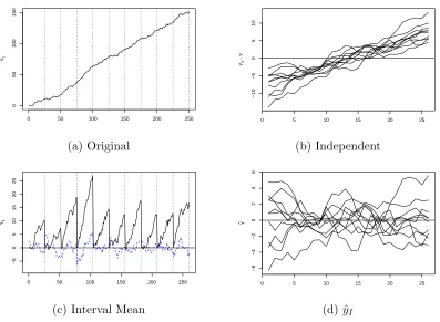
In Figure 3.1, we illustrate the process of data transformation for a simple AR (1) model under the null hypothesis that ρ = 1. In the upper plot, the solid line denotes the original series with T = 250, and the dotted line is the independent transformation withm= 10 andn = 25 where the error process{ǫ}is generated from
N(0, 1). The lower plot draws the independent transformed data in each interval over
j = 0,1,2,· · · ,25. This plot is the same plot as the panel unit root data with 10 individuals over 25 time points. As can be seen, the plot spreads out as n increases, which display a property of a unit root process, that is, the increase of variance.
Table 3.1: Data Transformation Process Original Data Double-index Independent
Transformation Transformation
Y11, Y12,· · · , Y1n 0, Y11, Y12,· · · , Y1n
Y0, Y1, Y2,· · · , YT ... ...
0 50 100 150 200 250
0
10
20
30
Yt
0 25 50 75 100 125 150 175 200 225 250
0
10
20
30
Yt
yij
(a) Original
5 10 15 20 25
−5
0
5
10
yij
(b) Transformation
3.1.2
Estimation and asymptotic results
The transformed model is the same form as in the panel data model so that the Pooled OLS (POLS) estimator for ρ is given by
ˆ
ρ =
Pm i=1
Pn
j=1yijyij−1
Pm i=1
Pn
j=1yij2−1
(3.23)
As mentioned in Chapter 2, we apply the sequential limits to obtain the limiting distribution of ˆρ. Under the null hypothesis thatρ= 1,yij−yi,j−1 =ǫij, so we obtain
the n√m-consistent ρ-statistic as in the panel unit root
n√m·(ˆρ − 1) = (
√
mn)−1Pmi=1Pnj=1yij−1ǫij m−1n−2Pm
i=1
Pn
j=1y2ij−1
(3.24)
The t-statistic is given by
tρ=
ˆ
ρ−1
q
ˆ
σ2/Pm i=1
Pn
j=1y2ij−1
= σ −2Pm
i=1
Pn
j=1yij−1ǫij ˆ
σ σ
q
σ−2Pm i=1
Pn
j=1yij2−1
(3.25)
These results imply that the POLS estimator adopting the sequential limit is “super-consistent” for n, and is asymptotically normally distributed as m → ∞ in contrast to the results of standard univariate unit root tests.
Lemma 3.1 Under the null hypothesis ρ= 1, for given Model M1,
ˆ
σ2 = 1
mn m X
i=1 n X
j=1
(yij −ρyˆ ij−1)2 p
Proof of Lemma 3.1
ˆ
σ2 = 1
mn m X i=1 n X j=1
(yij −ρyˆ ij−1)2
= 1 mn m X i=1 n X j=1
(ǫij −(ˆρ−ρ)yij−1)2
= 1 mn m X i=1 n X j=1
ǫ2ij+ (ˆρ−ρ)2 1
mn m X i=1 n X j=1
y2ij−1−2(ˆρ−ρ) 1
mn m X i=1 n X j=1
yij−1ǫij
since ǫij =yi,j −ρyij−1,
= 1 mn m X i=1 n X j=1 ǫ2
ij−(ˆρ−ρ)
1 mn m X i=1 n X j=1
yij−1ǫij
= 1 mn m X i=1 n X j=1
ǫ2ij−(ˆρ−ρ)√1 m 1 √ mn m X i=1 n X j=1
yij−1ǫij
since ˆρ−ρ=Op(m−1/2n−1) and √mn1 Pmi=1Pnj=1yij−1ǫij =Op(1),
= 1 mn m X i=1 n X j=1
ǫ2ij+Op(
1
mn) p −→σ2.
Theorem 3.1 (Levin and Lin, 1992)Under the null hypothesis thatρ= 1and
Asump-tion 3.1, as (n, m)seq → ∞, the following hold:
n√m·(ˆρ − 1) ⇒ N 0, 2 (3.27)
tρ ⇒ N 0, 1
(3.28)
Proof of Theorem 3.1
n√m·(ˆρ − 1) =
1 n√m
Pm i=1
Pn
j=1yij−1ǫij 1 n2 m Pm i=1 Pn
j=1y2ij−1
=
1
√mPmi=1 1nPnj=1yij−1ǫij
1 m
Pm i=1 n12
Pn
j=1yij2−1
By applying sequential limits, the n limit is
n→∞ =⇒
1
√m12Pmi=1(W2
i(1)−1) 1 m Pm i=1 R1 0 W 2 i(r)dr
where =⇒ denotes weak convergence and Wi(r), i = 1,2,· · · , m, are independent
standard Wiener processes. See Chan and Wei (1987, 1988) and Hall and Heyde (1980) for the derivation of the functional of Wiener process. Since R01W2
i(r)dr are
well defined random variables by Fuller (1996) in the sense that they have the finite first two moments and theWi are independent of each other,
1 m m X i=1 Z 1 0
Wi2(r)dr −→p E
Z 1
0
W2(r)dr
= 1
2 asm→ ∞
1 2√m
m X
i=1
W2
i (1)−1 d
−→ N
0, 1
2
as m→ ∞
Therefore, by the Slutsky theorem, this sequential limit approach gives
n√m ρˆ − 1 =⇒ N 0, 2
The tρ-statistic is given by tρ=
ˆ
ρ−1
q
ˆ
σ2/Pm i=1
Pn
j=1yij2−1
=
Pm i=1
Pn
j=1yij−1ǫij
ˆ
σqPmi=1Pnj=1y2 ij−1
=
1 n√m
Pm i=1
Pn
j=1yij−1ǫij/σ2 ˆ σ σ q 1 mn2 Pm i=1 Pn
j=1y2ij−1/σ2 d
−→ N 0, 1
In the last equality, we used Lemma 3.1 and the above asymptotic results.
Alternatively, we can use exact moments for interval i which appear in Dickey (1976). Especially, the exact moments obtained are very useful to study the asymp-totic behavior when the size of interval, n, is fixed. In that case, the asymptotics are functionals ofn as mentioned in chapter 2. Define
Nin=
1
nσ2 n X
j=1
yij−1ǫij, and Din=
1
n2σ2 n X
j=1
Table 3.2: Moments of an Simple AR(1) Model (Dickey, 1976)
E(Ni) = 0 E(Nin) = 0
E(N2
i) = 12n(n−1)σ4 E(Nin2) = 12 +o( 1 n)
Var(Ni) = 12n(n−1)σ4 Var(Nin) = 12 +o(1n)
E(Di) = 12n(n−1)σ2 E(Din) = 12 +o(1n)
E(D2
i) = 121n(n−1)(7n
2 −7n+ 4)σ4 E(D2
in) = 127 +o( 1 n)
Var(Di) = 13n(n−1)(n2−n+ 1)σ4 Var(Din) = 13 +o(n1)
Cov(Ni, Di) = 13(n−1)n(n−2)σ4 Cov(Nin, Din) =o(n1)
The moments for Ni and Di are listed in the above table which is also useful for the
case that m → ∞and n is fixed.
Using these results, we can obtain the asymptotic results:
n√m·(ˆρ − 1) = (
√
mn)−1Pmi=1Pnj=1yij−1ǫij m−1n−2Pm
i=1
Pn
j=1yij2−1
= m
−1/2Pm i=1Nin m−1Pm
i=1Din
= Nm
Dm d
→ N(0,2) as m→ ∞
and
tρ=
ˆ
ρ−1
q
ˆ
σ2/Pm i=1
Pn
j=1yij2−1
= m−
1/2Pm i=1Nin ˆ
σ σ
p
m−1Pm i=1Din
d
−→N(0,1).
Since we know that 1 √ m m X i=1 Nin d −→N
0,1
2 , 1 m m X i=1 Din p
−→ 12, and σˆ2 −→p σ2,
3.1.3
Behavior under the alternative
Now we study the statistical behavior of the POLS estimator under the alternative
|ρ| < 1. To this end, we first check whether or not the estimator of ρ for Model 1 (3.21) is consistent.
ˆ
ρ=
Pm i=1
Pn
j=1(Yi,j−1−Yi−1,n)(Yij −Yi−1,n)
Pm i=1
Pn
j=1(Yi,j−1−Yi−1,n)2
with Y0,n = 0
=
Pm i=1
Pn
j=1(YijYij−1 −YijYi−1,n−Yij−1Yi−1,n+Yi2−1,n) Pm
i=1
Pn
j=1(Yij2−1−2Yij−1Yi−1,n+Yi2−1,n)
= 1 mn Pm i=1 Pn
j=1(YijYij−1−YijYi−1,n−Yij−1Yi−1,n+Yi2−1,n) 1
mn Pm
i=1
Pn
j=1(Yij2−1−2Yij−1Yi−1,n+Yi2−1,n)
p
−→ (ρ+ 1)2γ γ0
0
= 1
2(ρ+ 1) where 1 mn m X i=1 n X j=1
YijYij−1 p
−→γ1 =ργ0
1 mn m X i=1 n X j=1
YijYi−1,n p
−→γj =ργj−1.
Under the null hypothesis ρ = 1, the POLS estimator of ρ is consistent, that is, ˆ
Next we study the limiting distribution of the POLS estimator under the alterna-tive. With simple algebra, we know thatρb−1−→p 21(ρ−1). Let us defineρ∗ = 1
2(ρ−1)
and ρb∗ =ρb−1. We consider the following regression
yij −yij−1 = (ρ−1)yij−1+ǫij.
Usingyij =Yij −Yi−1,n, it can be rewritten as
Yij −Yij−1 = (ρ−1)(Yij−1−Yi−1,n) +ǫij.
Then the POLS estimator ofρ∗ is given by
b ρ∗ =
Pm i=1
Pn
j=1(Yij −Yij−1)(Yij−1−Yi−1,n) Pm
i=1
Pn
j=1(Yij−1−Yi−1,n)2
.
In order to obtain asymtotic normality, we subtractρ∗ = 1
2(ρ−1) from the both sides
b
ρ∗−ρ∗ =
Pm i=1
Pn
j=1{Yij −Yij−1−ρ∗(Yij−1−Yi−1,n)}(Yij−1−Yi−1,n)
Pm i=1
Pn
j=1(Yij−1−Yi−1,n)2
=
Pm i=1
Pn
j=1{ǫij + (ρ−1)Yij−1−ρ∗(Yij−1 −Yi−1,n)}(Yij−1−Yi−1,n)
Pm i=1
Pn
j=1(Yij−1−Yi−1,n)2
= {ǫij +ρ ∗(Y
ij−1+Yi−1,n)}(Yij−1−Yi−1,n) Pm
i=1
Pn
j=1(Yij−1−Yi−1,n)2
=
Pm i=1
Pn
j=1{ǫij +ρ∗(Yij−1+Yi−1,n)}(Yij−1−Yi−1,n)
Pm i=1
Pn
j=1(Yij−1−Yi−1,n)2
As in the panel data framework, multiplying√mn on the both sides yields
√
mn ρb∗−ρ∗=
1 √ mn Pm i=1 Pn
j=1{ǫij +ρ∗(Yij−1+Yi−1,n)}(Yij−1−Yi−1,n)
1 mn Pm i=1 Pn
j=1(Yij−1−Yi−1,n)2
Since we know the asymptotic behavior of the denominator, if we know the asymptotic behavior of the numerator, then we obtain the limiting distribution of the pooled OLS estimator of ρ under the alternative. The numerator, say Nmn, can be rewritten as
Nmn =
1 √ mn m X i=1 n X j=1
ǫij(Yij−1−Yi−1,n) +ρ∗
1 √ mn m X i=1 n X j=1
(Yij2−1−Yi2−1,n)
def
= A + ρ∗B.
In Assumption 3.2, we assume that E{|ǫij|2+δ} ≤ M < ∞ for some δ > 0. In
order to obtain the result in part A, especially, we assume that E{ǫ4
ij} = ησ4 < ∞
as in Theorem 6.2.1 of Fuller (1996, p. 314). Also, to prove part B, we assume that E{ǫ6
ij}=ξσ6 <∞as in Theorem 6.2.3 of Fuller(1996, p.317) where ifǫij are normally
distributed, thenη= 3. That is, to obtain the probability limit of the estimator of the autocovariance function for a stationary series, we need the finite fourth moment, and we need the finite sixth moment for the probability limit of the variance-covariance estimator of autocovariance function.
For part A, since ǫij is independent of (Yij−1−Yi−1,n)∀i, j, E(A) = 0 and
1
n n X
j=1
Eǫ2ij(Yij−1−Yi−1,n)2 = 1 n n X j=1 E
ǫ2ij(Yi,j2−1+Yi2−1,n)−2ǫ2ijYi,j−1Yi−1,n = 1 n n X j=1
2(γ0 +γj−1)σ2 (∵
X
h
|γh|<∞)
= 2γ0σ2+O(n−1).
Hence, we have the following result 1 mn m X i=1 n X j=1 ǫ2
ij(Yij−1−Yi−1,n)2 p
−→2γ0σ2 =
2 1−ρ2σ
Thus we obtain the asymptotic distribution for A as follows:
A −→d N
0, 2
1−ρ2σ 4
.
For part B, by WLLN we obtain the asymptotic results for the first two moments: 1 mn m X i=1 n X j=1
(Yij2−1−Yi2−1,n) = 1
mn m X i=1 n X j=1
Yi,j2−1− 1 m
m X
i=1
Yi2−1,n
p −→ 1 n n X j=1
EY2
i,j−1−EYi2−1,n = 0.
1
n n X
j=1
E(Yij2−1−Yi2−1,n)2 = 1
n n X
j=1
[E(Yij4−1) + E(Yi4−1,n)−2E(Yij2−1Yi2−1,n)]
= 1
n n X
j=1
[2E(Yij4−1)−2E(Yij2−1Yi2−1,n)]
= 1 n n X j=1
2·3{E(Yij2−1)}2−2{E(Yij2−1)E(Yi2−1,n) + 2(E(Yij−1Yi−1,n))2} = 1 n n X j=1
(4γ02−4γj2)
= 4γ02+O(n−1) uniformly in i.
Hence, 1 mn m X i=1 n X j=1
(Yij2−1−Yi2−1,n)2 −→p 4γ02.
For B we have the asymptotic distribution
B −→d N
0, 4
(1−ρ2)2σ 4
.
Now we should check the correlation between A and B. 1
n n X
j=1
E[ǫij(Yij−1−Yi−1,n)(Yij2−1−Yi2−1,n)] = 0.
1 mn m X i=1 n X j=1
This result implies that A and B are asymptotically uncorrelated.
E(AB) = 0.
The result that Aand B are asymptotically individually normal does not directly imply the bivariate asymptotic normality of the pair of (A, B). In this case, we can prove the asymptotic normality via the Cramer-Wold device. Let λ = (λ1, λ2)′ 6= 0 and Xn = (A, B)′. ThenλXn
d
−→λX where
X∼N
0, 2
1−ρ2σ
4+ 4
(1−ρ2)2σ 4
.
Using the preceding results, it follows rather easily that
λXn = √1 mn m X i=1 n X j=1
λ1ǫi,j(Yi,j−1−Yi−1,n) +λ2(Yi,j2−1−Yi2−1,n)
converges to a normal random variable with mean 0 and varianceλ21Var(A)+λ22Var(B),
thus establishing the joint asymptotic normality of A and B and in particular for
λ1 = 1 and λ2 =ρ∗ it establishes the asymptotic distribution of Nmn.
Therefore,
Nmn d
−→ N
0, 2
1−ρ2σ 4+ 1
4(ρ−1)
24γ2 0
=N
0, 2
1−ρ2σ
4+ 1
(1 +ρ)2σ 4
=N
0, 3 +ρ
(1−ρ2)(1 +ρ)σ 4
Finally, by the Slutsky theorem we obtain the limiting distribution ofρb∗ −ρ∗
√
mn ρb∗−ρ∗ −→d N
0, (3 +ρ)(1−ρ)
4
For this regression model, the mean squared error is given by
ˆ
σ2 = 1
mn m X i=1 n X j=1
[Yij −Yij−1−(ˆρ−1)(Yij−1−Yi−1,n)]2
= 1 mn m X i=1 n X j=1
[ǫij+ (ρ−1)Yij−1−(ˆρ−1)(Yij−1−Yi−1,n)]2
= 1 mn m X i=1 n X j=1
[ǫij+ (ρ−ρˆ)Yij−1+ (ˆρ−1)Yi−1,n]2
= 1 mn m X i=1 n X j=1 ǫij +
ρ+ 1
2 −ρˆ
(Yij−1−Yi−1,n) +
ρ−1 2
(Yij−1+Yi−1,n) 2 = 1 mn m X i=1 n X j=1
ǫ2ij +
ˆ
ρ− ρ+ 1
2 2 1 mn m X i=1 n X j=1
(Yij−1−Yi−1,n)2
+
ρ−1
2 2 1 mn m X i=1 n X j=1
(Yij−1+Yi−1,n)2
−2
ρ−1
2
ˆ
ρ− ρ+ 1
2 1 mn m X i=1 n X j=1
(Yij2−1−Yi2−1,n) + other cross product terms
p
−→σ2+ 2
1−ρ
2
2
γ0 =
3 +ρ
2(1 +ρ)σ
2
Now we can obtain the asymptotic distribution of the t-statistic
t= s ρb∗−ρ∗
ˆ
σ2·
Pm
i=1
Pn
j=1(Yi,j−1−Yi−1,n)2 −1
=
√
mn(ρb∗−ρ∗)
s
ˆ
σ2·
1 mn Pm i=1 Pn
j=1(Yi,j−1 −Yi−1,n)2
−1
d
where
V = 2(1 +ρ) 3 +ρ
2 1−ρ2
(3 +ρ)(1−ρ)
4 = 1.
Therefore, we have the following results:
√
mn(ρb∗−ρ∗) −→d N
0, (3 +ρ)(1−ρ)
4
forρ∗ = 1
2(ρ−1)
t −→d N(0, 1).
3.2
Model 2: Intercept AR (1) model
In this section we consider an AR (1) model with intercept under the alternative hypothesis given by
Yt = α(1−ρ) + ρYt−1 + ǫt (3.30)
where t= 1,2,· · ·, T and ǫt follows Asummption 3.1. Using the double-index
trans-formation we can rewrite Equation (3.30):
Yi,j = α(1−ρ) + ρYi,j−1 + ǫij, (3.31)
wheret = (i−1)n+j, i= 1,· · · , m, j = 1,· · · , n,and mn=T. Now, under the null hypothesis that ρ= 1 the independent transformation for Equation (3.31) yields
yi,j = yi,j−1 + ǫi,j (3.32)
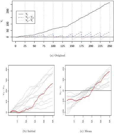
where yi,j = Yi,j −Yi−1,n. The last value subtraction for the independent
Equation (3.32) model M2-GD or M2-ID which are exactly the same as model M1. Thus, for Equation (3.32) we can use the methodology for the simple AR (1). This method is adopted by Breitung and Meyer (1994) for panel unit root tests so they could avoid the bias in the estimate of ρ due to the incidental parameter.
0 50 100 150 200 250
0
10
20
30
Yt
0 25 50 75 100 125 150 175 200 225 250
0
10
20
30
Yt yij
5 10 15 20 25
−5
0
5
10
yij
(a) Original (b) Independent
5 10 15 20 25
−6
−4
−2
0
2
4
6
Yij
−
Yi
5 10 15 20 25
−5
0
5
10
Yij
−
Y
(c) Interval Mean (d) Global Mean
Figure 3.2: Transformation of Intercept AR (1) Model
![Figure 4.5: Empirical Size of t(0.05) with Break in Level in M2-G [T=100, m=5]](https://thumb-us.123doks.com/thumbv2/123dok_us/1601009.1197799/108.612.137.518.106.436/figure-empirical-size-break-level-m-g-t.webp)