DOI: 10.1534/genetics.107.071696
A Bayesian Multilocus Association Method: Allowing for Higher-Order
Interaction in Association Studies
Anders Albrechtsen,*
,†,‡,1Sofie Castella,*
,‡Gitte Andersen,
‡Torben Hansen,
‡Oluf Pedersen
‡and Rasmus Nielsen
†*Bioinformatics Centre, University of Copenhagen, 2100 Copenhagen, Denmark,†Department of Biostatistics, University of Copenhagen, 2100 Copenhagen, Denmark and‡Steno Diabetes Center, 2820 Gentofte, Denmark
Manuscript received February 4, 2007 Accepted for publication March 31, 2007
ABSTRACT
For most common diseases with heritable components, not a single or a few single-nucleotide polymorphisms (SNPs) explain most of the variance for these disorders. Instead, much of the variance may be caused by interactions (epistasis) among multiple SNPs or interactions with environmental conditions. We present a new powerful statistical model for analyzing and interpreting genomic data that influence multifactorial phenotypic traits with a complex and likely polygenic inheritance. The new method is based on Markov chain Monte Carlo (MCMC) and allows for identification of sets of SNPs and environmental factors that when combined increase disease risk or change the distribution of a quantitative trait. Using simulations, we show that the MCMC method can detect disease association when multiple, interacting SNPs are present in the data. When applying the method on real large-scale data from a Danish population-based cohort, multiple interactions are identified that severely affect serum triglyceride levels in the study individuals. The method is designed for quantitative traits but can also be applied on qualitative traits. It is computationally feasible even for a large number of possible interactions and differs fundamentally from most previous approaches by entertaining nonlinear interactions and by directly addressing the multiple-testing problem.
M
OST common diseases are multifactorial andinfluenced by several factors that can be of both genetic and environmental origin (Landerand Schork 1994; Weiss 1994). The more prevalent of these dis-orders include cancer, diabetes, obesity, hypertension, and premature cardiovascular morbidity and mortality. Numerous genetic variations have been implicated as major pathogenic factors in various Mendelian disor-ders. However, the success in identifying the genetic factors underlying complex traits has at times been limited (Glazieret al. 2002; Hirschhornet al. 2002). Many studies have been challenged by a presumed low effect of each genetic variant, small study populations, confounding effects such as population stratification, and, possibly, the use of highly simplistic genetic models. Even though conditions such as diabetes harbor strong genetic components, not a single or a few single-nucleotide polymorphisms (SNPs) explain most of the genetic variance for these disorders (Risch and
Merikangas 1996). It is hypothesized that much of
the genetic variation may be caused by the interaction (epistasis) of multiple SNPs and interaction with en-vironmental conditions (Cordell 2002). The disease penetrance associated with each allele is low and the
impact of genetic components may vary depending on
the genetic and environmental background (Carlson
et al. 2004). Great progress has been achieved in the last few years using simple linear models (Cockerhamand Zeng1996; Falconer1996; Schaidet al. 2002; Baker 2005). However, for large-scale data the methods often cannot detect interactions that are believed to have a substantial impact on the development of complex diseases (Culverhouseet al. 2004), because the models include only linear interactions and because the sol-utions that have been developed to address the multiple-testing problem lead to a drastic reduction in the statistical power (Cardonand Bell2001). When mod-eling all the possible interactions between environmen-tal factors and many SNPs at different loci using classical methods, the number of necessary parameters becomes very large as the number of SNPs increases (Nelson et al. 2001; Culverhouseet al. 2004). This is one of the main reasons why SNP–SNP interactions and SNP– environment interactions are rarely modeled in associ-ation studies (Carlborgand Haley2004) even though these interactions are essential in uncovering the eti-ological background for complex diseases.
Some of the more successful methods for incorporat-ing higher-order interactions are based on clusterincorporat-ing algorithms. The combinatorial partitioning method
(Nelson et al. 2001) was one of the first methods to
1Corresponding author:The Bioinformatics Centre, Universitetsparken 15, 2100 Copenhagen, Denmark. E-mail: [email protected]
model higher-order interactions without any main effect. This method evaluates all possible partitions and is not computationally feasible for large-scale data. The popular multifactor-dimensionality reduction (MDR)
(Ritchie et al. 2001) for binary traits reduces the
number of partitions by labeling the possible combina-tions as either high risk or low risk. The results are then evaluated through cross-validation or permutation test-ing, which compensates for multiple testing.
Several methods based on regression and classifica-tion trees allow for some interacclassifica-tions and are extremely fast (Breimanet al. 1984; Freundand Schapire1997; Huanget al. 2004). One of these is the random forest method (Breiman2001). This method uses a bootstrap sample of the data to construct a tree and uses the nonsampled (called ‘‘out of bag’’) data for cross-validation. Multiple bootstrap samples are used to construct aforest
of trees and the significance of each parameter is de-termined from the out-of-bag samples.
We propose using Markov chain Monte Carlo (MCMC) to overcome some of the problems described. MCMC is a stochastic computational approach that is very useful in Bayesian statistics where it can be used to estimate the posterior distribution of the parameters using Monte Carlo integration. This is achieved by generating sam-ples from an ergodic Markov chain that has the same stationary distribution as the posterior distribution. MCMC provides a convenient method for dealing with a large parameter space when only parts of the posterior distribution are of interest. The new method explores sets of effects (risk sets) that increase the risk, or the phenotypic value, for individuals who fulfill the crite-rion defined by the sets. A risk set may contain one or more genetic or environmental conditions. The MCMC method then provides a probability that a particular risk set exists,i.e., that the conditions specified by the risk truly cause an increase in the phenotypic value or a higher disease risk. Methods that explore such a large range of models (multiple combinations of effects) often have very little power because they do not effi-ciently combine the evidence for association from dif-ferent models. The new Bayesian method addresses this problem by combining information from many differ-ent models, for example, by evaluating the effect of all possible interactions when testing the effect of a single SNP. The method is described inmaterials and methods and the software for the method is called BAMSE and can be found at http://biostat.ku.dk/ande/BAMSE
MATERIALS AND METHODS
Risk sets:In the context of this method, a risk set is a subset of the parameter space that partitions the individuals on the basis of their genotypes and environmental factors. Let V denote all possible sets of SNPs and environmental factors (discrete or continuous). Let the jth group of individuals whose genetic and environmental profiles fit a risk setTjV
denote a potential risk groupGj. Individuals not in any of the
risk groups are placed inG0. We set the upper bound,mr, on the number of risk sets so that the number of risk setsnm2{0,
1,. . .,mr} is finite. An example of a risk set could be {weight.
90 kg, sex is male, SNP3 is a heterozygote} and the individuals who fit this description constitute a risk group. Given a quantitative trait yifor individual i2 Gjand assuming that
the trait for every individual in a given risk group is in-dependent and normally distributed with equal variance, the observations yi are modeled as yi
Pnm
j¼0Ifi2GjgNðaj;s 2Þ, where nm is the number of risk sets, and I is the
indica-tor function. Let mbðT1;T2;. . .;Tnm;a0;a1;a2;. . .;anm;sÞ be a state from the spaceM. If the phenotype is binary (case– control design) the phenotype is modeled using a binomial distribution whereajis the probability for being a case in the
jth risk group.
Each risk setTjdefines a genetic and environmental profile
and all individuals must fit this profile to be part of the associated risk groupGj. The space of thelth componentTjlfor
thejth risk set is defined asVland it is a finite discretization of
a compact subspace ofRor a finite subset ofN, depending on
thelth parameter. For example, a SNP parameter has seven states given that individuals who are heterozygous and ho-mozygous for major and minor alleles are all present in the sample (see Equation A4). This corresponds to one state for each possible combination of genotypes. For the continuous-risk parameters, such as environmental factors, a thresholdt can be defined that excludes individuals with observations that exceed this threshold. The space is defined as eitherTl
j ¼{a:
a.t} orTl
j ¼{a:a,t}. Let thejth risk setTjbe the set of the
risk parametersTj ¼ fTj1;T
2
j ;. . .;T np
j gfornpparameters.
In some instances an individual may fit several risk sets. In this case an individual is placed in the risk group with the highest meanai. Since not all of the observations (SNPs and
environmental factors) are necessarily thought to affect the trait in a causative combination, not all of them need to define a risk set. Therefore, only someTl
j’s are needed to restrict the
jth risk group and the number of components, henceforth called the active risk components (for risk setj), will there-fore be restricted tona2{1, 2,. . .,ma}, wherema#np. This means that a risk set can be restricted to a maximum ofma active components. If only thekth component is active for the jth risk set thenTj ¼ fTj1;T
2
j;. . .;T k j;. . .;T
np
j g ¼ fV1;V2;. . .;
Vk1;Tjk;Vk11;. . .;Vnpg, which means that only thekth
com-ponent restricts thejth risk group.
Priors: The means,aj’s, for the risk sets are assumed to be
normally distributed with the empirical averageyas mean and a variance calculated from the length of the range of the observed valuesRso thataN(j,k1), wherekis a multiple of
R2andj¼y. The prior forkis the same prior in Richardson
and Green(1997).
For the quantitative traits the variance is chosen to be uniformly distributed on (0,‘). The priors for the distribution of the active risk components are uniformly chosen. The priors for the number of active risk componentsnaand the number of risk sets nm are chosen to be geometrically
distributed, pnaGðpaÞ and pnmGðprÞ, respectively. Both distributions are normalized to sum to one. The priors for components defining the SNP and environmental factors are chosen to be uniformly distributed.
The Markov chain: The chain is updated using the Metropolis–Hasting algorithm with acceptance probability
aðm;m9Þ ¼min 1;Lðm9Þpðm9Þqðmjm9Þ LðmÞpðmÞqðm9jmÞ
ð1Þ
L(m) is the likelihood for statem. The method is implemented so that the parameters are updated one at a time when pos-sible. However, when updating the number of active compo-nents or the number of risk sets, updates of several parameters must simultaneously be proposed. A new risk set can be pro-posed with a random choice of parameters or a risk set can be deleted, which is sometimes called the death/birth move. Details regarding the proposal algorithm are provided in the
appendix.
The posterior probability of a certain risk setTk can be
approximated as
pðTkjdataÞ ¼
1 N B
XN
i¼B
IfTk2mig;
whereBis the burn-in,Nis the number of iterations, andmi
is theith sampled state. Likewise, the posterior probability for the number of risk sets being equal toxis
pðnm¼xjdataÞ ¼
1 N B
XN
i¼B
Ifx¼nmig;
wherenmi is theith sampled number of risk sets andIis the indicator function. This probability can be used to evaluate whether there are any factors, genotypical or environmental, that affect the trait.
Simulations:To evaluate the sensitivity and selectivity of the method several simulations were performed under different genetic models. Simulations were performed assuming 500 unrelated individuals with 20 uncorrelated SNPs and assum-ing equal variance for affected and unaffected individuals. The frequency of the minor allele was chosen to be 0.2 for all the SNPs and the mean phenotypical value for unaffected indi-viduals was 100 with a standard deviation of 10. The same variance was chosen for the affected individuals but with vary-ing means. However, in two genetic scenarios linkage disequi-librium (LD) was simulated using coalescent simulations based on the ms program (Hudson2002), and the
frequen-cies of the SNPs were thus random variables. In these simulations, a region was simulated under a neutral infinite size model assuming a crossover at rate of 1/4N0for a 50,000-bp-long segment per generation, where N0 is the effective population size. A random selection of 20 SNPs with a minor allele frequency .0.05 was included in the nonepistatic scenario. For the epistatic scenario 20 SNPs were selected from two regions and a SNP with a minor allele frequency between 0.17 and 0.23 from each region was selected as a susceptibility SNP. Throughout, a burn-in of 10,000 iterations and a run time of 100,000 were chosen for the MCMC analysis by examining the convergence of the likelihood score and using thepotential scale reduction factor(PSRF), also called the ‘‘shrinking factor’’(Gelmanand Rubin1992), for the
param-eters that are always sampled. The shrinking factor was visualized at several intervals of the chains as recommended in Brooksand Gelman(1998). The risk parameters that were
frequently, but not always, sampled were transformed into Bernoulli variables (0 for sampled and 1 for nonsampled) and then tested in the same manner as the other parameters.
To evaluate the power of the MCMC-based method com-pared with that of a linear model and random forests, sensitivity and selectivity were calculated for the three methods under different genetic models. The result is presented as ROC curves for general use of the MCMC method, the random forest, and a one-locus linear model. We evaluate the ability of the methods to detect any effect in the data and to identify specific susceptibility loci.
The sensitivity and selectivity for the linear model is calculated using anF-test comparing the full one-locus model
to the null model of no genetic impact (three parametersvs. one parameter). For the MCMC method, the posterior prob-ability of at least one risk set½p(nm.0jdata)was used to
detect an effect in the data and the posterior probability of SNP i belonging to a risk set divided by the posterior probability for there being at least one risk set ½p(Ti Tj
data)/p(nm.0jdata)was used for identifying the
suscepti-bility SNPs. The estimated increase in mean squared error was used for identifying SNPs using the random forest method and the estimated explained variance was used to detect an effect in the data. The random forest implementation in the statistical software R version 2.3.1 was used. Five hundred trees for each data set were chosen and seven variables were ran-domly sampled as candidates at each split. When identifying the SNPs, the susceptibility SNPs act as the true positives and the other SNPs as false positives. For detecting an effect in data, the simulations were compared with another set of simulations without any genetic effect. For the linear model the best (lowest)P-values from the two sets of simulations were com-pared. The same data sets were used for the three methods.
Gene–gene–environment interactions affecting serum tri-glycerides:Inter99 is a population-based cohort of 6741 individ-uals randomly recruited using the central person registry from the western part of Copenhagen County (Glu¨ meret al. 2003).
Only individuals with Danish ancestry by self report were in-cluded. A second group of individuals consisting of type 2 diabetes patients was recruited at Steno Diabetes Center. An oral glucose tolerance test was used to determine the glucose toler-ance status of each individual according to the WorldHealth
Organization(1999): normal glucose tolerant (NGT), impaired
fasting glycemia (IFG), impaired glucose tolerance (IGT), and type 2 diabetes (T2D). Smoking habits were quantitated on the basis of interviews and questionnaires for the Inter99 cohort.
RESULTS
SNPs, the effect is even more pronounced. The differ-ence in power is manyfold at a low false-positive rate. However, in the presence of LD the advantage of the MCMC is somewhat reduced, which is due to the vary-ing SNP frequency in the simulations.
In general, the MCMC-based method outperforms the normal linear model when dealing with interac-tions, especially multiple combinations of interacinterac-tions, while the linear model in some cases may perform slightly better when dealing with a single susceptibility SNP with additive effects. The random forest method performs better than the linear model at detecting interact-ing SNPs, but much worse at detectinteract-ing the effect of a sinteract-ingle locus. On the basis of a limited number of simulations the three methods seem fairly robust against phenocopy and small departures from normality (data not shown).
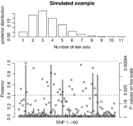
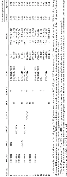
To illustrate the efficacy of the method when the number of individuals is large we simulated 100 SNPs from five regions and 5000 unrelated individuals with effect sizes so that the linear model could not achieve significance after Bonferroni correction. Phenotypes were simulated on the basis of a second- and a third-order interaction, i.e., five susceptibility SNPs. A de-scription of the simulated data and the result from the simulation can be seen in Figure 3 and Table 1. Figure 3
and Table 1 show that the MCMC method provides very strong evidence for association½p(nm.0)¼1and that the method easily identifies the five susceptibility SNPs and the two specific combinations. The sampling from the stationary distribution starts within a few thousand iterations, which is,1 min on a standard PC.
Gene–gene–environment interactions affecting se-rum triglycerides:To illustrate the method we applied it to the data described inmaterials and methodsfor a
1131 T.C polymorphism in theAPOA5gene and a
250 G . A, an IVS1 1 49 C . T, and a Ser215Asn
polymorphism in the LIPC gene. APOA5 and LIPC
are two of several genes where common alleles, many in high linkage disequilibrium, have shown a strong association with serum lipids such as triglycerides and cholesterol (Kaoet al. 2003; Laiet al. 2003; Kloset al. 2005; Olivaet al. 2005). It has been hypothesized that APOA5 interacts with lipoprotein lipases that hydrolyze the apolipoproteins. Furthermore, it has been shown that APOA5 binds to the lipases (Merkelet al. 2005). APOA5 has been shown to be expressed only in the liver
(Pennacchioet al. 2001), where the hepatic lipase
en-coded byLIPCis also found. Hepatic lipase hydrolyzes triglycerides and has been shown to enhance the uptake of lipoproteins (Thuren2000). The effect of the1131
Figure 1.—ROC curves for the three
T.C polymorphism in theAPOA5promoter has shown a consistent association with serum triglycerides in various studies in different ethnic groups. Recently, a small association study ( Jianget al. 2005) indicated that plasma glucose levels may interact with anAPOA5 poly-morphism, giving higher plasma triglyceride levels among type 2 diabetic patients, but failed to show any interactions among nondiabetic subjects. Association studies of theAPOA51131 T.C variant in the Inter99 cohort have shown that the effect on serum triglyceride of the deleterious allele is modulated by other factors that affect serum triglyceride levels (G. Andersen, T. Sparsø,
A. Albrechtsen, S. Castella, C. Glu¨ mer, K. Borch
-Johnsen, T. Jørgensen, R. Nielsen, T. Hansen and
O. Pedersen unpublished results). These factors
in-clude glucose tolerance status, gender, and smoking habits. The interactions were found using a linear model with two-way interaction terms. Using a linear model it was not possible to include all possible interaction terms among all factors. No interaction was found with the three SNPs inLIPCand theAPOA5variant using a linear model. However, since the effect of the APOA5 poly-morphism is strongly modulated through glucose toler-ance status, gender, and smoking habits it is possible that an association with serum triglycerides can be observed
only through higher-order interactions. Therefore, the
APOA5 variant, the three LIPC variants, sex, smoking habits, and glucose tolerance status were included in the MCMC method. The adjustment factors age and body mass index (BMI) were also included, assuming a linear relationship. The glucose tolerance status and the smok-ing habits each have four categories (NGT, IFG, IGT, and T2D and never smoked, used to smoke, occasional smoker, daily smoker, respectively). Both environmental factors were assumed to be discrete ordinal variables.
We applied the MCMC method two times on 5300 individuals without missing data from the Inter99 co-hort using 5,000,000 iterations in each run. The two chains gave similar results and the parameters sampled in each iteration can be seen in Figure 4. Convergence diagnostics were performed using the method of
Gelmanand Rubin(1992) and the multivariate
shrink-ing factor was,1.01. The serum triglyceride levels were logarithmically transformed and two extreme outliers were excluded (6–8 SD from the mean after transforma-tion). The method sampled 6–14 risk sets (see Figure 4B), where 10 was the most frequent sample. All the factors used in the method were frequently sampled (see Figure 4C). Not surprisingly, the environmental factors were sampled in each iteration.
Figure 2.—ROC curves for the three
The final results can be seen in Table 2. Even though there was no main effect of the threeLIPCvariants, they all show an association with serum triglyceride levels in combination with both genetic and environmental fac-tors. Using the same criteria for the risk sets as seen in Table 2, plots for the genotypes and mean serum tri-glyceride levels whenLIPC250 G.A,LIPCIVS1149 C.T, orLIPCSer215Asn were part of the criteria are shown in Figure 5. The presence of several factors in a risk set does not necessarily imply an interaction but could also be additive effects between the factors. One of the risk sets that indicates a strong epistatic effect is the risk set consisting of smoking nonnormal glucose tolerance status (IFG, IGT, T2D) individuals with a combination ofAPOA5andLIPCIVS1149 C/T alleles (see Figure 5A). The (unadjusted) P-values using a linear model for these stratifications of the data are also Figure3.—Results for a simulated scenario with 100 SNPs
and 5000 unrelated individuals. Five 500,000-bp-long regions were simulated using the ms program. SNPs with a minor al-lele frequency of,0.05 and the SNPs in high LD (r2.0.95)
were removed. Then 20 SNPs were randomly selected from each region and one SNP from each of the five regions with a minor allele frequency between 0.17 and 0.23 was chosen as a susceptibility SNP. Phenotypes were simulated so that the in-dividuals with at least one minor allele at SNP8 and SNP34 had a phenotype drawn from N(103, 100) and individuals with at least one minor allele at SNP46, SNP77, and SNP82 had a phenotype drawn fromN(104, 100). Individuals with minor alleles at all five susceptibility SNPs had a phenotype drawn fromN(107, 100) and individuals without any of the two combinations had a phenotype drawn from N(100, 100). The prior for the MCMC method is chosen asj¼y, k¼100=R2, s U(0, ‘), p
naGð0:5Þ, and pnmGð0:5Þ. The posterior distribution for the number of risk sets is shown at the top and the posterior probabilities for a SNP pa-rameter being part of a risk set is shown at the bottom. Also, theP-values for the full single-locus linear model are shown as x’s and the dashed and dotted lines denoteP-values of 0.05 and 0.0005, respectively. The frequently sampled risk sets can be seen in Table 1.
shown for illustration purposes. For risk set 6 we tested for epistasis between these SNPs for the smoking IFG, IGT, and type 2 diabetics using a linear model with covariates for being carriers of the minor alleles. To verify this, using standard methods, we followed up this finding by also performing the test for interactions on another cohort of 1008 IFG, IGT, and type 2 diabetic individuals consisting mostly of type 2 diabetics. A total of 683 of the individuals were smokers. TheP-value of replication was 0.003 and it was the same allele combi-nation that gave heightened serum triglyceride levels. It should be noted that most of the individuals in the follow-up group are under treatment, which may po-tentially influence the results.
DISCUSSION
The MCMC approach appears to have overcome many of the major difficulties in modeling higher-order interactions in large-scale population-based data. For many SNPs no method can explore all of the possible interactions. However, the MCMC method uses the marginal effects for a low-order interaction to find the higher-order interactions. For example, if a fifth-order interaction exists in the data, then the phenotypical mean of the group of individuals with three of the five factors will probably be different from that for the rest of the individuals. The Markov chain will then spend more time in this state and by exploring the ‘‘local’’ area will
find the fifth-order interaction (see appendix for up-dates of the Markov chain).
A related fully Bayesian MCMC method, called
BAMA, has recently been developed (Kilpikari and
Sillanpaa 2003). However, there are some important
differences between our method and BAMA. The BAMA method assumes no interactions among loci, that all alleles have different effects, and that the effects from each locus are additive. Another related method is the Monte Carlo version of logic regression (Kooperberg
and Ruczinski 2005). This method uses Boolean
ex-pressions to model covariates in a linear model and thus allows for higher-order interactions. Monte Carlo logic regression uses maximum-likelihood estimates for the coefficients in the model. The current MCMC method models all multiple combinations of SNPs and does not assume any linear relationship between the effects of any combination of SNPs and environmental factors. How-ever, our method does allow adjustment factors to be included in the model if a linear relationship is assumed. We chose to compare our method with random forest because it does not make any linear assumptions.
Computational speed: The speed of the algorithm is highly dependent on the number of individuals and the number of sampled risk sets. For the simulated data, where the number of sampled risk sets is rather low and the number of individuals is few (500), application of the method takes ,1 min, while under the larger simulation condition (5000 individuals, 100 SNPs) each Figure4.—Result for the
MCMC analysis of SNPs and environmental factors af-fecting triglyceride. A total of 5300 individuals with three SNPs and three en-vironmental factors were tested against fasting serum triglycerides. The triglyc-eride levels were logarith-mically transformed before testing. j¼y, k¼100=R2, s U(0, ‘),nm G(0.5),
replicate takes a few minutes. When the method was applied on the Inter99 sample, the MCMC method found multiple risk sets defined by up to four factors, which could not be accomplished using most other methods. For example, modeling all possible interactions using a standard linear model would entail including 2592 parameters in the model.
Power:The main advantage of the MCMC method is that it allows multiple effects simultaneously, thereby reducing the variance and allowing information to be pooled among effects. This gives the method more power than the linear models in most genetic scenarios when dealing with multiple susceptibility SNPs. Simu-lations showed that the MCMC can have more than twice the power of the linear model to detect two two-way interactions when the average number of false positives is low (,1). When there are interactions pres-ent in the data, then many combinations of SNPs will, to some extent, be associated with the trait even without any main effect. However, when compensating for mul-tiple testing only information from the most strongly associated combination is used. The MCMC method combines information from many SNPs and risk sets in the calculation of the posterior probability and, thus, if many combinations are associated, the MCMC
method compensates for multiple testing at a much lower cost.
While no method can entirely circumvent the prob-lem of ‘‘the curse of dimensionality’’ (Bellman1961), our simulations show that the new method is feasible for at least 100 SNPs. Although it may not be worthwhile to entertain the possibility of three-way or four-way inter-actions in data sets with thousands of SNPs (there are 1011 possible three-way interactions for 10,000 SNPs),
the method can still be efficiently applied to such large data sets if the state space is constrained to exclude high-order interactions.
The new method is too slow for modeling, for ex-ample, 500,000 SNPs even without interactions. None-theless, while we see our method as most suitable for candidate gene studies, we also note that application in large-scale genomewide studies is possible. For these studies, we recommend using the method by applying it independently to different genic regions, in addition to using standard methods. If multiple SNPs within the same genic region have an effect, such an application of the method should greatly increase the mapping power compared to methods that analyze each SNP separately.
Priors and assumptions: The MCMC method seems to perform well under a range of different genetic Figure5.—Bar plots for some of the risk sets
models and does not assume the same genetic model for the different risk sets. The factors used in the method can be either biallelic SNPs or environmental risk fac-tors that can be continuous or discrete ordinal. All environmental factors are treated as binary traits, but the threshold that divides the data need not be defined in advance. The environmental factor can be included in two ways, either as the measured values or trans-formed to the sorting order of the values. By using the latter, the prior for the number of individuals included or excluded from a risk set is then uniformly distributed where, if the actual values were used, the prior for the threshold would be uniformly distributed in the range of the values of the environmental factor. The priors for the mean of each risk set (h,k) can have a great effect on the posterior distribution of the number of risk sets (see, for example, Richardson and Green 1997 with discussion). If the mean is chosen as the midrange of the trait instead of the empirical average, the MCMC method is likely to predict a higher number of risk sets. This, however, is highly dependent onk(the prior var-iance for the means) or the multiple ofk, where a small multiple gives a rather flat prior distribution.
Caveats: Label switching, where different risk sets partition the data in the same way, is a potential problem in this MCMC method. Defining the risk sets to have a higher mean than the set of individuals not in a risk set
"i:ai.a0largely eliminates this problem. However, a label-switching problem can still remain. For example, a risk group might contain all or none of the individuals, which means the data are partitioned in the same way as if there were no risk sets. This problem can be addressed in the calculation of posterior probabilities by appro-priate editing of the MCMC output data, and it is, in any case, partially alleviated by assigning low prior proba-bility to states with a high number of risk sets. In our implementation of the method, the number of non-empty risk sets is calculated.
It is important to note that the posterior probabilities estimated using the MCMC method do not have a frequentist interpretation. For example, in repeated simulations without a genetic effect, a posterior proba-bility of.0.4, for there being at least one risk set, was virtually never observed. Practitioners desiring to report a frequentistP-value can do so by applying the method in combination with a standard permutation procedure. For small data sets, similar to the data sets simulated in this article, such permutations are easily completed on a single stand-alone computer. Permutation testing on large and complex data sets would require access to a cluster of processors.
The MCMC method can detect a range of different genetic effects, whether they be main effects, epistatic, gene–environment, or a mixture of them. In most ge-netic scenarios with multiple causative factors, the method has equal or more power to detect an effect and identify the causal combination of genetic factors
than the more conventional linear model. The method can model higher-order interactions and find significant reproducible combinations of both genetic and environ-mental factors that influence serum triglyceride levels.
We thank Charlotte Glu¨ mer, Knut Borch-Johnsen, and Torben Jørgensen for generously supplying the Inter99 data. This work was supported by the Danish research counsel and by National Institutes of Health grants NIGMS R01HG003229, U01HL084706.
LITERATURE CITED
Baker, S. G., 2005 A simple loglinear model for haplotype effects in a case-control study involving two unphased genotypes. Stat. Appl. Genet. Mol. Biol.4:14.
Bellman, R. E., 1961 Adaptive Control Processes. Princeton University Press, Princeton, NJ.
Breiman, L., 2001 Random forest. Mach. Learn.45:5–32. Breiman, L., J. H. Friedman, R. A. Olshenand C. J. Stone, 1984
Clas-sification and Regression Trees, Ed. 1. Wadsworth, Belmont, CA. Brooks, S. P., and A. Gelman, 1998 General methods for
monitor-ing convergence of iteractive simulations. J. Comp. Graph. Stat. 7:434–455.
Cardon, L. R., and J. I. Bell, 2001 Association study designs for complex diseases. Nat. Rev. Genet.2:91–99.
Carlborg, O¨ ., and C. S. Haley, 2004 Epistasis: too often neglected in complex trait studies. Nat. Rev. Genet.5:618–625.
Carlson, C. S., M. A. Eberle, M. J. Rieder, Q. Yi, L. Kruglyaket al., 2004 Selecting a maximally informative set of single-nucleotide polymorphisms for association analyses using linkage disequilib-rium. Am. J. Hum. Genet.74:106–120.
Cockerham, C. C., and Z. B. Zeng, 1996 Design III with marker loci. Genetics143:1437–1456.
Cordell, H. J., 2002 Epistasis: what it means, what it doesn’t mean, and statistical methods to detect it in humans. Hum. Mol. Genet. 11:2463–2468.
Culverhouse, R., T. Kleinand W. Shannon, 2004 Detecting epi-static interactions contributing to quantitative traits. Genet. Epi-demiol.27:141–152.
Falconer, M., 1996 Introduction to Quantitative Genetics, Ed. 4. Longman, New York.
Freund, Y., and R. E. Schapire, 1997 A decision-theoretic generaliza-tion of on-line learning and an applicageneraliza-tion to boosting. J. Comput. Syst. Sci.55:119–139.
Gelman, A. F., and D. Rubin, 1992 Inference from iterative simu-lation using multiple sequences (with discussion). Stat. Sci.7: 457–511.
Glazier, A. M., J. H. Nadeauand T. J. Aitman, 2002 Finding genes that underlie complex traits. Science298:2345–2349.
Glu¨ mer, C., T. Jorgensenand K. Borch-Johnsen, 2003 Prevalences of diabetes and impaired glucose regulation in a Danish popula-tion: the Inter99 study. Diabetes Care26:2335–2340.
Green, P. J., 1995 Reversible jump Markov chain Monte Carlo com-putation and Bayesian model determination. Biometrika 82: 711–732.
Hirschhorn, J. N., K. Lohmueller, E. Byrneand K. Hirschhorn, 2002 A comprehensive review of genetic association studies. Genet. Med.4:45–61.
Huang, J., A. Lin, B. Narasimhan, T. Quertermous, C. A. Hsiung et al., 2004 Tree-structured supervised learning and the genetics of hypertension. Proc. Natl. Acad. Sci. USA101:10529–10534. Hudson, R. R., 2002 Generating samples under a Wright-Fisher
neutral model of genetic variation. Bioinformatics18:337–338. Jiang, Y. D., C. J. Yen, W. L. Chou, S. S. Kuo, K. C. Lee et al., 2005 Interaction of the G182C polymorphism in the APOA5 gene and fasting plasma glucose on plasma triglycerides in type 2 diabetic subjects. Diabet. Med.22:1690–1695.
Kao, J.-T., H.-C. Wen, K.-L. Chien, H.-C. Hsuand S.-W. Lin, 2003 A novel genetic variant in the apolipoprotein A5 gene is associated with hypertriglyceridemia. Hum. Mol. Genet.12:2533–2539. Kilpikari, R., and M. J. Sillanpaa, 2003 Bayesian analysis of
Klos, K. L. E., S. Hamon, A. G. Clark, E. Boerwinkle, K. Liuet al., 2005 APOA5 polymorphisms influence plasma triglycerides in young, healthy African Americans and whites of the CARDIA study. J. Lipid Res.46:564–571.
Kooperberg, C., and I. Ruczinski, 2005 Identifying interacting SNPs using Monte Carlo logic regression. Genet. Epidemiol. 28:157–170.
Lai, C.-Q., E.-S. Tai, C. E. Tan, J. Cutter, S. K. Chewet al., 2003 The APOA5 locus is a strong determinant of plasma triglyceride con-centrations across ethnic groups in Singapore. J. Lipid Res.44: 2365–2373.
Lander, E. S., and N. J. Schork, 1994 Genetic dissection of com-plex traits. Science265:2037–2048.
Merkel, M., B. Loeffler, M. Kluger, N. Fabig, G. Geppert et al., 2005 Apolipoprotein AV accelerates plasma hydrolysis of triglyceride-rich lipoproteins by interaction with proteogly-can-bound lipoprotein lipase. J. Biol. Chem.280:21553–21560. Nelson, M. R., S. L. Kardia, R. E. Ferrelland C. F. Sing, 2001 A combinatorial partitioning method to identify multilocus geno-typic partitions that predict quantitative trait variation. Genome Res.11:458–470.
Oliva, C. P., L. Pisciotta, G. LiVolti, M. P. Sambataro, A. Cantafora et al., 2005 Inherited apolipoprotein A-V deficiency in severe hypertriglyceridemia. Arterioscler. Thromb. Vasc. Biol.25:411– 417.
Pennacchio, L. A., M. Olivier, J. A. Hubacek, J. C. Cohen, D. R. Cox et al., 2001 An apolipoprotein influencing triglycerides in hu-mans and mice revealed by comparative sequencing. Science 294:169–173.
Richardson, S., and P. J. Green, 1997 On Bayesian analysis of mix-tures with an unknown number of components (with discus-sion). J. R. Stat. Soc. Ser. B59:731–792.
Risch, N., and K. Merikangas, 1996 The future of genetic studies of complex human diseases. Science273:1516–1517.
Ritchie, M. D., L. W. Hahn, N. Roodi, L. R. Bailey, W. D. Dupontet al., 2001 Multifactor-dimensionality reduction re-veals high-order interactions among estrogen-metabolism genes in sporadic breast cancer. Am. J. Hum. Genet.69:138–147. Schaid, D. J., C. M. Rowland, D. E. Tines, R. M. Jacobsonand G. A.
Poland, 2002 Score tests for association between traits and haplotypes when linkage phase is ambiguous. Am. J. Hum. Genet. 70:425–434.
Scheet, P., and M. Stephens, 2006 A fast and flexible statistical model for large-scale population genotype data: applications to inferring missing genotypes and haplotypic phase. Am. J. Hum. Genet.78:629–644.
Thuren, T., 2000 Hepatic lipase and HDL metabolism. Curr. Opin. Lipidol.11:277–283.
Weiss, K. M., 1994 Genetic Variation and Human Disease. Cambridge University Press, Cambridge/London/New York.
World Health Organisation, 1999 Definition, diagnosis and classification of diabetes mellitus and its complications: report of a WHO consultation. Part 1: diagnosis and classification of di-abetes mellitus. Technical Report. World Health Organisation, Geneva.
Communicating editor: M. Nordborg
APPENDIX
Pseudocode: The algorithm can be written in pseu-docode as
runtime¼N
while (runtime – –){ update SNP parameters
update environmental parameters update a mean for a random risk set update adjustment factors
update the number of active risk components
update the positions of the active risk component update the missing genotypes
update a mean for a random risk set
update the number of risk sets using delete or create mean_update¼5
while(mean_update – –){ update of variance
update a mean for a random risk set }
sample the parameters }
where Nis the number of iterations. In each update a proposal update is either accepted or rejected.
Update of means: Since a reasonable choice for a mean should be no higher than the maximum pheno-typic value maxpand no lower than the minimum phe-notypic value minp, the parameter space for a mean is defined as½minp, maxp. The proposed meana9i of risk setiis sampled either fromN(j,k1) or fromU(min
p, maxp). The latter is used when the acceptance rate of the updates falls below a specified threshold. This may typically happen when the Markov chain visits states with many risk sets.
The acceptance probability for this update is
aðm;m9Þ ¼min 1;Lðm9ÞqðaiÞpða9iÞ
LðmÞqða9iÞpðaiÞ
: ðA1Þ
To avoid some of the problems with label switching the risk sets T1;T2;. . .;Tnm can be chosen to have a
higher mean thanT0. When updating the mean for one of the risk sets it is restricted to ½a0, maxp andT0is restricted to½minp;minni¼m1ai.
Update of the variance: The variance is updated by simulating a uniformU(sw,s1w) random variable, where w is some specified constant. If the proposed value,s9, is outside (0,‘),i.e., less than zero, it ismirrored
back into the space
s9¼ s$ s$,0
s$ s$2 ð0;‘Þ;
ðA2Þ
wheres99is the unmirrored proposal variance sampled fromU(sw,s1w). This ensures thatq(mjm9)¼q(m9j m) and reversibility.
The acceptance probability for this update is
aðm;m9Þ ¼min 1;Lðm9Þ LðmÞ
ðA3Þ
because the prior densities are uniformly distributed.
Update of adjustment factors: This update is per-formed similarly to the update of the variance, but without any restrictions inR.
1 fWTg 2 fHEg
3 fHOg
4 fWT;HEg
5 fHE;HOg
6 fWT;HOg
7 fWT;HE;HOgðcalled nonactiveÞ; ðA4Þ
where partition 7 allows all genotypes. Updates are proposed by sampling from their uniform prior density
U{1, 2, 3,. . ., 6} and the acceptance probability is the same as (A3). The updates for being active are proposed separately.
The environmental parameters allow the individuals to enter risk sets if they have environmental values that are below or higher than a given thresholdtij. Theith environmental parameter takes values in the interval between the observed minimum and maximum envi-ronmental values. Again the proposals are sampled from their uniform prior density and the acceptance proba-bility becomes (A3).
Updating the number of active risk components: In the presence of many environmental and genetic fac-tors, a random risk set is likely to result in an empty risk group. Therefore, it will in most cases lead to significant savings of computational time to define an upper limit for the number of components that are active in a risk set. The maximum number of active components in a risk set,ma, can be defined by the user.
The probability of deactivating a given active risk component for risk seti when there currently are nai
active components is defined as 1/nai and the
probabil-ity of activating a given inactive risk component is 1=ðnpnaiÞ. The acceptance probability for
deactivat-ing a risk component becomes
aðm;m9Þ ¼min 1; pðn9aiÞpadðn9aiÞLðm9Þnai
pðnaiÞpadðnaiÞLðmÞðnpnai11Þ
;
ðA5Þ
where p(nai) is the prior for the number of active
components in theith risk set andpadðnaiÞ ¼
np
nai
is
the prior for the distribution of the active components. The acceptance probability for activating a risk component is
aðm;m9Þ ¼min 1;pðn9aiÞpadðn9aiÞLðm9ÞðnpnaiÞ
pðnaiÞpadðnaiÞLðmÞðnai11Þ
:
ðA6Þ
Updating the active risk component:Risk sets are also updated by simultaneously proposing a deactivation of one component and an activation of another
compo-nent. The components chosen to be activated or de-activated are chosen with equal probability. Because the priors are also uniformly distributed, the resulting ac-ceptance probability is given by (A3).
Updating the number of risk sets:To allow different combinations of genotypic and phenotypic factors to have different effects, we allow multiple risk sets with different means. Using reversible jumps (Green1995), the Markov chain can jump between parameter spaces of different dimensionality. To ensure reversibility, a random componentcis used so that the mapping from
mtom9isone-to-one. The mapping, when creating a new risk set, is defined as
a9n9m
T9n9m
a$
T$ s9
0 B B B B @
1 C C C C
A¼
1 0 0 0 0
0 1 0 0 0
0 0 1 0 0
0 0 0 1 0
0 0 0 0 1
0 B B B B @
1 C C C C A
c1 c2
a
T
s 0 B B B B @
1 C C C C
A; ðA7Þ
where 1 is the identity matrix, 0 is a zero matrix,
a9¼ ða$;a9n9mÞ, and T9¼ ðT$;Tn99mÞ. The Jacobian for
this mapping is the identity matrix and thus does not need to be included in the acceptance probability.
The number of active risk components in the new risk setn9aiis uniformly proposed from {1, 2,. . .,ma}, and the positions of each active risk component are also chosen with equal probability. When proposing a new risk set the mean of the new risk set, the SNPs, and the en-vironmental factors are sampled from their prior den-sity. The acceptance probability then reduces to
aðm;m9Þ ¼min 1;Lðm9Þpðn9mÞpðn9aiÞ
LðmÞpðnmÞqðn9aiÞ
; ðA8Þ
where pðn9aiÞ is the prior for the number of active
components in the proposed risk set (i) andqðn9aiÞis the
probability of proposing this number.
Updating missing genotypes: The priors for the missing genotypes are calculated on the basis of the fre-quencies of the observed genotypes, pj, at locusj and assuming Hardy–Weinberg equilibrium
pðgj¼iÞ ¼Ii¼0p2j 1Ii¼12pjð1pjÞ1Ii¼2ð1pjÞ2; ðA9Þ
whereiis the number of minor alleles andgjis the state of the genotype.
All the missing genotypes for one SNP are updated at the same time and proposed from the prior distribution so that the acceptance probability is given by (A3).