Nonlinear optimal control of plate structures using magnetostrictive actuators

(1)

Nonlinear Optimal Control of Plate

Structures Using Magnetostrictive Actuators

William S. Oates

1

_{and Ralph C. Smith}

2

Center for Research in Scientific Computation Department of Mathematics

North Carolina State University Raleigh, NC 27695

Abstract

A nonlinear optimal control method is developed for magnetostrictive actuators used to actively attenuate plate vibration. Significant improvements in vibration control can be achieved when the magnetostrictive actuators are driven at moderate to high field levels. This results in nonlinearity and hysteresis which cannot be effectively compensated using linear control theory. This issue is addressed by introducing a homogenized energy model that accounts for nonlinear, hysteretic constitutive behavior into the control design. Numerical examples illustrate significant improvements in vibration attenuation when the nonlinear control method is implemented.

Keywords: Hysteresis, magnetostriction, nonlinear control, optimal control

1. Introduction

Smart materials offer several advantages over conventional actuation systems such as high energy density, compactness, and broadband capability which has provided numerous novel devices and adaptive structures. One of the major challenges associated with implementing these materials is determining how to compensate for nonlinear and hysteretic constitutive behavior. Nonlinear control laws are often needed at moderate to high drive levels to meet increasingly stringent performance requirements in applications such as atomic force microscopy, morphing aircraft structures, high speed milling, and precision optics.

A significant amount of research in developing smart material devices and adaptive structures has focused on determining robust control design. Many works assume linear material behavior [3, 5, 18, 19] which works well in low to moderate drive regions. In moderate to high drive regimes, however, inherent hysteresis can create a phase lag between the input field and the actuation response. This can destabilize a system if the control law is not robust. To address this issue, several techniques have been proposed such as inverse compensators [16], neural network controllers [2], and Preisach models [10].

In this paper, a model-based nonlinear optimal control method is developed for smart material structures. Although this method can be applied to a variety of smart material systems, the control design is demonstrated on an elastic plate structure that uses nonlinear magnetostrictive actuators to actively dampen vibration. This work is an extension of a previous model [20] for controlling beam dynamics that used a domain wall constitutive model [13]. The current control design is extended to two-dimensional plate structures and uses a homogenized free energy model [22] to predict magnetostrictive constitutive behavior. The domain wall model is effective in modeling symmetric loop behavior, but does not guarantee biased minor loop closure typically observed in materials with negligible thermal relaxation and rate dependent hysteresis. Although the domain wall model

can be modified to include closure of minor loop hysteresis, it requiresa priori knowledge of the turning points

which precludes use in feedback control since the turning points are not typically known in advance. Minor loop closure can be obtained using Preisach models, but these models typically require a large number of unphysical parameters to accurately predict minor hysteresis. The homogenized free energy model addresses closure of minor hysteresis loops by incorporating certain physical parameters at multiple length scales to predict macroscopic constitutive behavior.

(2)

The development of the optimal control method is presented as follows. Section 2 briefly describes the homogenized free energy model. The magnetically actuated plate structure is developed in Section 3. In Section 4, the optimal control problem is discussed. First the linear optimal control problem is summarized to motivate the need for nonlinear control at moderate to high drive levels. Nonlinear optimal control is then shown to compensate for hysteresis.

2. Homogenized free energy model

A one-dimensional magnetostrictive constitutive model can be used to model the actuator device. The typical magnetostrictive transducer employed in the structural control problem is described in detail by Hall and Flatau [11]. The homogenized energy model assumes linear stress-strain behavior and nonlinear, hysteretic field-magnetization behavior. Details regarding the model development are give in [22] and only a summary of the constitutive model is presented here. The model is based on a Gibbs energy relation at the lattice or mesoscopic length scale. Local magnetic moments are assumed to be either aligned or diametrically opposed to the magnetic field. The model is extended to the macroscopic length scale through a stochastic homogenization technique.

The following constitutive law is used in developing the control law,

σ(t) =YMε(t)−a1[M(H+HI;Hc, ξ)]2(t) (1)

[M(H+HI;Hc, ξ)] (t) =

Z ∞

0 Z ∞

−∞

ν1(Hc)ν2(HI)£M(H+HI;Hc, ξ)¤(t)dHIdHc (2)

whereσ(t) is uniaxial stress, ε(t) is the elastic strain,YM _{is the elastic modulus at constant magnetization,}_a

1

is the magnetostrictive coefficient, andM is the magnetization. In (2),M is the local magnetization,H is the

applied field,HI is the interaction field,Hcis the coercive field andξdenotes the initial distribution of magnetic

variants. The interaction field represents local material inhomogeneities. The probability density functions of

the coercive field and local field interactions are given by ν1(Hc) and ν2(HI). The change in stress on the

Terfenol actuators is restricted to small plate vibration therefore, magnetomechanical coupling is neglected in (2).

The local magnetizationM is given by,

M(H+HI;Hc, ξ) =χm(H+HI) +MRδ(H+HI;Hc, ξ) (3)

where δ = 1 if the local magnetization variant MR is in the positive direction and δ = −1 if oriented in the

negative direction. The magnetic susceptibility is defined byχm.

The stochastic homogenization technique is used to construct a macroscopic constitutive model that ac-counts for a myriad of local material inhomogeneities such as intergranular residual stress, mismatches in grain orientation, and impurities. As detailed in [22], the coercive field and interaction densities are taken to be

ν1(Hc)ν2(HI) =c1c2e−[ln(Hc/Hc)/2c]

2

e−H2

i/2b2 (4)

whereHcis the average coercive field,cquantifies the coercive field variability,bis the variance of the interaction

field, and c1 and c2 are scaling parameters. The proposed densities give reasonable estimation of major and

minor hysteresis. They are implemented to reduce parameter estimation. Model comparison to experimental results can be found in [22].

The local magnetization MR given in (3) will switch when magnetic variants diametrically opposed to the

effective field (He = H +HI) reach the coercive field. The switching behavior is modeled by introducing a

(3)

−40 −20 0 20 40 −150

−100 −50 0 50 100 150

Magnetic Field (H) kA/m

Magnetization (M) kA/m

−400 −20 0 20 40

200 400 600 800 1000 1200

Magnetic field H (kA/m)

microstrain

(µε)

(a) (b)

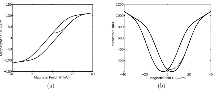
Figure 1: (a) Macroscopic magnetizationM versus magnetic fieldH computed using (2), and (b) microstrainµ²versus magnetic fieldH computed from (1) under zero external stress.

3. Structural model

The structural model consists of a thin plate coupled with Terfenol transducers placed along the fixed edges of the plate. Eight transducers are oriented in four pairs where each pair is connected by a moment arm that is perpendicular to the plate. Diametrically out-of-phase currents applied to each actuator couple generate a moment on the plate. This system is based on a previous experimental arrangement for assessing vibration control [7].

3.1 Plate with nonlinear actuators

The thin plate structure can by modeled using classical plate theory [24]. Deformation is assumed to be

small which allows the equation of motion describing transverse plate displacementwto decouple from in-plane

displacements. Since the control problem is concerned with attenuating vibration transverse to the plate, the

dynamic equation forwis only given.

The strong form of the equation of motion can be determined from force and moment balances,

ρ∂

2_w

∂t2 −

∂2_Mint x

∂x2 −

∂2_Mint y

∂y2 =

∂2_Mmag x

∂x2 +

∂2_Mmag y

∂y2 (5)

whereρdenotes the density of the plate and Mint_x andMint_y include the internal elastic and damping moment

components in thexandydirections, respectively. The in-plane moment componentMint_xy is zero in the present

case since the plate is isotropic and no twisting moments are applied. The external moments generated by the

Terfenol transducers are represented byMmag_x and Mmag_y in thexand y directions, respectively. A detailed

description of the equations describing the moment-displacement relations are given in [21]. Spatial variations in density, moment of inertia and compliance near the Terfenol transducers and connecting moment arms are assumed to be negligible.

Boundary conditions are specified to determine the transverse displacement in (5). The plate is clamped along the fixed edges [x,0] and [0, y] and free along [`x, y] and [x, `y] where the plate length and width are given

by`xand`y, respectively.

The external moment generated by the Terfenol actuators is given by,

(4)

where KM = a1AmagEM(h/2 +`r) andM1(i)(t) and M (i)

2 (t) are the magnetization for each of the four (i=1

. . . 4) top and bottom actuator pairs, respectively. HereAmag is the cross-section of the Terfenol rod,his the

plate thickness, and `r is the length of the moment arm. The characteristic function χrod is equal to one in

regions where the moment arm is attached to the plate and zero otherwise. The moment is applied in thex

direction along the fixed edge [0, y] and in they direction along [x,0]. Since the actuator strain is quadratic, a

nonzero moment requires a biasing magnetic fieldHbias. The time varying component of the control inputHe(t)

is opposite in sign on each actuator pair. The total magnetic field input isH(t) =He(t) +Hbias. This reduces

the number of control inputs from eight to four.

The equation of motion given by (5) can be rewritten in the weak form for numerically implementation and is given by (7)

Z

Ω µ

ρ∂

2_w

∂t2Φ− M

int x

∂2_Φ

∂x2 − M

int y

∂2_Φ

∂y2 ¶

dω=

Z

Ω µ

Mmag_x ∂

2_Φ

∂x2 +M

mag y

∂2_Φ

∂y2 ¶

dω (7)

where Φ∈H2

0(x, y).

3.2 Approximation method

The plate geometry is approximated using cubic B-splines to determine the optimal control input. Cubic Hermites could also be used but they require approximately twice the number of unknown coefficients. Details describing the attributes of cubic B-splines as well as comparisons to cubic Hermites are given in [21]. The cubic

B-splines are defined over the plate geometry, Ω = [0, `x]×[0, `y]. The plate is discretized over the points given

byxm=mhx and ym =nhy with hx= _N`x_x, hy = _N`y_y and m= 0, ..., Nx andn = 0, ..., Ny. The cubic spline

product space is defined by,

Φ(x, y) =φ(x)φ(y) (8)

The approximate solution to (7) is subsequently given by

w(t, x, y) =

Nω

X

k=1

wk(t)Φk(x, y) (9)

whereNω= (Nx+ 1)(Ny+ 1) andwk(t) are the displacements determined from the weak form of the model.

An ODE model is obtained by rewriting the weak form of the model as a set of first order differential equations

˙

y(t) =Ay(t) + [B(u)](t)

y(0) =y0.

(10)

where y(t) = [w1(t),· · ·, wNω(t),w˙1(t),· · ·,w˙Nω(t)]. The system matrix A contains the mass, stiffness and

damping relations of the plate, whereas the matrixB(u) contains the nonlinear and hysteretic magnetostictive

behavior. Details regarding the relations between the system matrices and the cubic B-splines are given in [20].

It should also be noted that the variableuis typically used in the control literature as the input. This variable

is equivalent to the magnetic fieldH(t) on the Terfenol transducer, butuwill be used in subsequent discussions

to be consistent with the control literature.

3.3 System parameters

Physical parameters employed in the control design are summarized in Table 1. The Terfenol material parameters are within the range obtained for model fits to an experimental transducer [6]. The plate modulus is typical for aluminum. The center location of the four actuator pairs was (0.105,0.2),(0.105,0.3),(0.15,0.105)

and (0.25,0.105) where the coordinate origin was located at the bottom left corner of the plate. The moment

arm is assumed to be rigid with length`r = 2.54 cm and square cross section area, Ar = 1 cm2. The

(5)

resolved by choosingNx=Ny = 4 in the frequency range considered. The dimension of the state vectory was

then 50×1 due to the inclusion of both displacement and velocity components.

Table 1: Parameters for the plate and Terfenol transducer.

Plate Terfenol Transducer

Ep = 4.1×1010N/m2 a1= 0.006N/A2

ρp= 2700kg/m3 c1=c2= 6.1×10−5m/A

cp= 2.5×105N s/m2 Hc= 3.3×103A/m

`x= 0.4m c= 0.4

`y= 0.6m b= 1.5×104A/m

γ= 0.18N s/m2 _M

s= 1.3236×105A/m

h= 0.0016m Amag= 0.0064m2

YM _{= 7}_.₀_×₁₀10_N/m2

4. Control methodology

The optimal control problem is first summarized to elucidate the technique used in developing the nonlinear control design [4, 14, 15, 17]. The general form of the finite dimensional control system under consideration is

˙

y(t) =f(y(t), u(t), t)

y(t0) =y0

(11)

where the states arey(t)∈lR2Nω _{and controls}_u₍_t₎_∈_lRp _where_p_{= 4 for the case of four actuator pairs driven}

diametrically out-of-phase. The model could have also been developed by letting p = 8, but as previously

mentioned in Section 3.1, a simplification is made to reduce model complexity. A cost functional is utilized to obtain the optimal control input,

J(u) = 1 2y

T₍_t

f)Πfy(tf) +

Z tf

t0

£

H(y, u, t)−λT₍_t_{) ˙}_y¤_dt ₍₁₂₎

where the positive definite matrix Πf penalizes large terminal values of the state,H(y, u, t) is the Hamiltonian,

andλ(t)∈lR2Nω _{is a set of Lagrange multipliers.}

The Hamiltonian is,

H(y, λ, u, t) = L(y, u, t) +λT_f₍_{y, u, t}₎

= 1

2

£

yT₍_t₎_Qy₍_t_{) +}_uT₍_t₎_Ru₍_t₎¤₊_λT_f₍_{y, u, t}₎

(13)

where the Lagrangian Lincludes the penalities on the states and inputs through the semi-definite maxtrix Q

and the positive definite matrixR.

The cost functional employed in (12) has been modified so that the optimization problem originally con-strained by (11) is now unconcon-strained by utilizing Lagrange multipliers (for details see [4, 14, 15]). The optimal

input is found by minimizingJ.

The optimal control problem requires solving the two point boundary value problem governed by (11) and the following adjoint or Lagrange multiplier condition,

˙

λ=−∂H

∂y λ(tf) = Πfy(tf).

(14)

(6)

∂H

∂u = 0 (15)

which results in the control relation

u∗₍_t_{) =}₋_R−1∂fT

∂u λ(t). (16)

4.1 Linear optimal control

It has been experimentally shown that a nearly linear relation exists between input current to the solenoid and strain output by the Terfenol transducer when the time varying input is small. In this situation, an approximate model can be attained through linearization about some biased input field. In the present model, a biased field of twice the coercive field is applied to the Terfenol rod. The magnetic susceptibility and remanent magnetization are constant under small changes in the input field. These values are determined from the constitutive law by

applying a small oscillating field with bias 2Hc. This ensures a self-consistent linear operatorB

B=−2KMMr(2Hc)χm(2Hc)~b (17)

whereMr(2Hc) is the biased magnetization at 2Hc,χm(2Hc) is the magnetic susceptibility at 2Hc,u(t) is the

magnetic field input, and~brepresents the location and direction of applied moments through integration of the

cubic B-spline functions.

With this approximation, the corresponding first-order system is

˙

y(t) =Ay(t) +Bu(t)

y(0) =y0.

(18)

The state constraint in (18) and adjoint condition in (14) yields the optimality system

"_y_˙₍_t₎

˙

λ(t)

#

=

"

A −BR−1_BT

−Q −AT

# "

y(t)

λ(t)

#

y(t0) =y0

λ(tf) = Πfy(tf)

(19)

and the control input is determined by solving an algebraic Ricatti equation [4] to yield

u∗₍_t_{) =}₋_Ky₍_t₎_. ₍₂₀₎

4.1.1 Numerical example – no external force

Active vibration control of the plate is illustrated by applying an external disturbance load to the plate from

tI = 0 sec to t0=0.45 sec. The external disturbance load is set to zero att0 and the control input is applied.

The initial conditiony0is defined as the state of the system att0.

Vibration attenuation is marginal when the Terfenol transducers are limited to small input fields. This

is illustrated in Figure 2(b) by plotting the plate displacement at the point [`x, `y]. The magenetic

field-magnetization response corresponding to the input control is illustrated in Figure 2(a).

(7)

5.5 6 6.5 7 7.5 16 17 18 19 20

6 6.5 7 7.5 16

17 18 19 20

Top Actuator Bottom Actuator

6.2 6.4 6.6 6.8 16

17 18 19 20

5.5 6 6.5 7 7.5 16

17 18 19 20

0 0.5 1 1.5 2 2.5 −25 −20 −15 −10 −5 0 5 10 15 20 25 Time (sec) Displacement (mm) (a) (b)

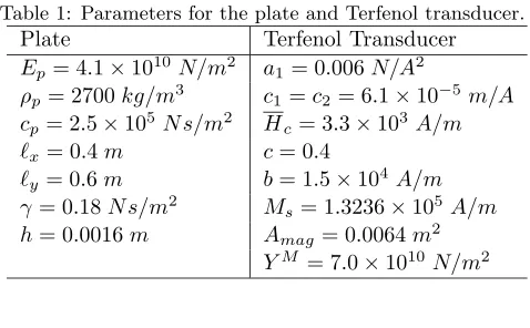
Figure 2: Performance of the linear feedback control law in the nonlinear model. The relationship between magnetic field and magnetization is given in (a) for each actuator pair. The resulting plate displacement for the uncontrolled ( ) and controlled response ( ) are given in (b).

2 4 6 8 10 20

25 30 35

4 6 8 10 20

25 30 35

5 6 7 8 20

25 30 35

4 6 8 10 20

25 30 35

Top Actuator Bottom Actuator

0 0.5 1 1.5 2 2.5 −25 −20 −15 −10 −5 0 5 10 15 20 25 Time (sec) Displacement (mm) (a) (b)

Figure 3: Linear feedback control law in the nonlinear model. The relationship between magnetic field and magnetization is given in (a) for each actuator pair. In this simulation,QandRwas increased to increase the input field. The resulting plate displacement for the uncontrolled ( ) and controlled response ( ) are given in (b).

4.2 Nonlinear control method

The nonlinear control method previously discussed by Smith [20] is applied to the Terfenol plate structure.

The nonlinear magnetostrictive material behavior contained within the input operator B(u) precludes

(8)

˙

z(t) =F(t, z)

E0z(t0) = [y0,0]T

Efz(tf) = [0,Πfy(tf)]T

(21)

wherez= [y, λ]T _and

F(t, z) =

"

Ay(t) + [B(u)](t)

−AT_λ₍_t₎₋_Qy₍_t₎

#

E0= "

I 0

0 0

#

, Ef =

"

0 0

0 I

#

.

(22)

Here I denotes a 2Nω×2Nω identity matrix whereNω denotes the number of basis functions employed in

the spatial approximation of the state variables given in Section 3.2. The optimal control satisfies

u∗(t) =−R−1[BT(u∗)](t)λ(t) (23)

where the nonlinear operatorB(u∗_{) is included in the optimal control input.}

As previously noted in [20], the solutions to the system given by (22) can be approximated through a variety of methods including finite differences and nonlinear multiple shooting [1]. To illustrate a finite difference

approach, a discretization of the time interval [t0, tf] with a uniform mesh having stepsize ∆t and points

t0, t1,· · · , tN = tf is considered. The approximate values of z at these times are denoted by z0,· · · , zN. A

central difference approximation of the temporal derivative then yields the system

1

∆t[zj+1−zj] =

1

2[F(tj, zj) +F(tj+1, zj+1)]

E0z0= [y0,0]T

EfzN = [0,Πfy(tf)]T

(24)

forj= 0,· · ·, N−1.

The determination of a solution vector zh = [z0,· · · , zN] to (24) can then be expressed as the problem of

findingzhwhich solves

F(zh) = 0. (25)

A quasi-Newton iteration of the formz_hk+1=zk

h+ξkh,whereξkh solves

F0(zkh)ξhk=−F(zkh), (26)

is used to approximate the solution to the nonlinear system given by (25). Direct solution of (26) is infeasible due to the large number of basis functions and time increments required to resolve the solution over a reasonable time interval. The structure of the Jacobian can be employed to reduce both memory and computational

requirements to the level of solving 4Nω×4Nω systems. This is accomplished by expressing the Jacobian in

terms of an analyticLU decomposition (see [20] for details).

The minimum of (25) was obtained by solving the LU decomposition problem by iteration. Convergence

was obtained by varying certain system parameters. The weighting matrixQ was reduced and the magnetic

bias in the nonlinear input matrixB(u∗_{) was increased to the saturation value (}_M

r=MR). Once the solution

began to converge, the weighting matrix Q was increased and the magnetic bias was reduced to ensure

(9)

4.2.1 Numerical example

The use of nonlinear control is shown to significantly enhance the ability to dampen vibration in the plate relative to the linear control design. In Figure 4, the same disturbance load is applied on the Terfenol plate

structure. When t0 = 0.45 sec, the disturbance is zero and control is instantaneously applied. By increasing

the penalty on the states throughQ, the control input reaches moderate to high drive levels. Although this

creates nonlinearity and hysteresis in the Terfenol transducers similar to that shown in Figure 3(a), the nonlinear control method provides reasonable compensation for this behavior.

2 4 6 8 10

15 20 25 30 35

4 6 8 10

15 20 25 30 35

Top actuator Bottom actuator

5 6 7 8

15 20 25 30 35

2 4 6 8 10

15 20 25 30 35

0 0.5 1 1.5 2 2.5

−30 −20 −10 0 10 20 30

Time (sec)

Displacement (mm)

(a) (b)

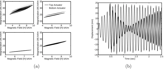
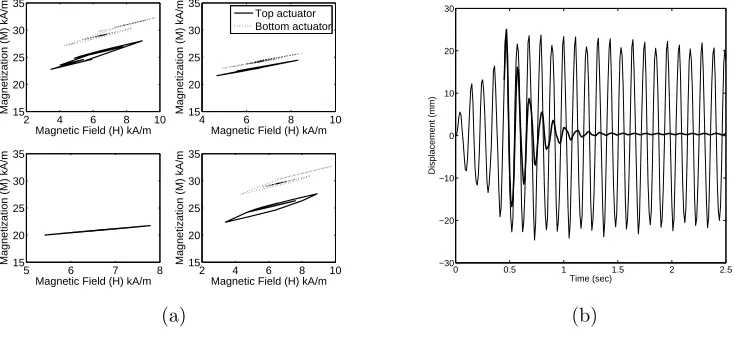
Figure 4: Nonlinear feedback control law for open loop control example. The relationship between magnetization and magnetic field is given in (a). The resulting plate displacement for the uncontrolled ( ) and controlled response ( ) are given in (b).

5. Concluding remarks

A nonlinear control design was extended to plate structures using multiple nonlinear magnetostrictive tran-ducers. It was illustrated that when the control input is limited to the linear region, marginal attenuation in vibration is achieved. When the control input is increased, minor hysteresis introduces a phase lag between the field input and the actuation response which cannot be compensated by the linear control method. The hystere-sis and nonlinearity are compensated through the use of an open loop nonlinear control method. This approach provides improved performance characteristics in attenuating vibration in the plate. Additional improvements can be made by implementing an appropriate feedback law to increase robustness in operating uncertainty. This issue is currently under investigation.

Acknowledgements

This research was supported in part by the Air Force Office of Scientific Research through the grant AFOSR-FA9550-04-1-0203

References

[1] U.M. Ascher, R.M.M. Mattheij and R.D. Russel,Numerical solution of boundary Value Problems for

Ordi-nary Differential Equations, SIAM CLassics in Applied Mathematics.

(10)

the Conference on Recent Advances in Adaptive and Senory Materials and their Applications, Technomic Publishing, Blacksburg, VA, April 27-29, pp. 465-479, 1992.

[3] M.D. Bryant and N. Wang, “Audio range controllability of linear motion Terfenol actuators,” J. Intell.

Mater. Syst. Struct.,5, pp. 431-436, 1994.

[4] A.E. Bryson and Y.-C. Ho,Applied optimal Control, Blasidell Publishing Company, Waltham, MA, 1969.

[5] J.L. Butler, “Application manual for the design of ETREMA Terfenol-D magnetostrictive transducers,” EDGE Technologies, Inc. Ames, IA.

[6] F.T. Calkins, R.C. Smith, and A.B. Flatau, “An energy-based hysteresis model for mangetostrictive

trans-ducers,” ICASE Report 97-60, IEEE Trans. Magn.,34(2), pp. 429-439, 2000.

[7] F.T. Calkins, R.L. Zrostlik, and A.B. Flatau, “Terfenol-D vibration control of a rotating shaft,” Proc. of the 1994 ASME Internation Mechanical Engineering Contgress and Exposition, Chicago, IL; Adaptive Structures

and Compositie Materials Analysis and Applications, AD-Vol.45, pp. 267-274, 1996.

[8] A.E. Clark, “Magnetostrictive rare earth-Fe2 compounds,” Chapter 7 inFerromagnetic Materials, Vol. 1,

E.P.Wohlfarth, editor, North-Holland Publishing Company, Amsterdam, pp. 531-589, 1980.

[9] A.B. Flatau and R. Kellog, “Blocked-force Charateristics of Terfenol-D Transducers,” J. Intell. Mater. Syst.

Struct.,15, pp. 117-128, 2004.

[10] W.S. Galinaaitis and R.C. Rogers, “Compensation for hysteresis using bivariate Preisach models,” Pro-ceedings of the SPIE , Smart Structures and Materials 1997: Mathematics and Control in Smart Structures, San Diego, CA March 1997.

[11] D.L. Hall and A.B. Flatau, “Analog feedback control for magnetostrictive transducer linearization,” J.

Sound Vib.,211(3), pp. 481-494, 1998.

[12] D.L. Hall and A.B. Flatau, “Nonlinearities, harmonics and trends in dynamics applications of Terfenol-D,”

Proc. of the SPIE Conference on Smart Structures and Intelligent Materials,1917Part 2, pp. 929-939, 1993.

[13] D.C. Jiles and D.L. Atherton, “Theory of the magnetomechanical effect,” J. Phys. D, Appl. Phys.,17, pp.

1265-1281, 1984.

[14] E.B. Lee and L. Markus, it Foundations of Optimal Control Theory, John Wiley and Sons, New York, 1967.

[15] F.L. Lewis and V.L. Syrmos,Optimal Control John Wiley and Sons, New York, 1995.

[16] J. Nealis and R.C. Smith, “Model-Based Robust Control Design for Magnetostrictive Transducers Operat-ing in Hysteretic and Nonlinear Regimes,” CRSC Technical Report: CRSC-TR03-25, IEEE Trans. Control Syst. Technol., submitted.

[17] E.R. Pinch,Optimal control and the Calculus of Variations, Oxford University Press, Oxford, 1993.

[18] J. Pratt and A.B. Flatau, “Development and analysis of a self-sensing magnetostrictive actuator design,”

J. Intell. Mater. Syst. Struct.,6(5), pp. 639-648, 1995.

[19] J. Pratt and A.H. Nayfey, “Boring-bar chatter control using a two-axes active vibration absorber scheme,” Proceedings of Noise-Con 97, The Pennsylvania State University, University Park, PA, June 15-17, pp. 313-324, 1997.

(11)

[21] R.C. Smith,Smart Material Systems: Model Development, SIAM, Philadelphia, PA, 2005.

[22] R.C. Smith, M.J. Dapino and S. Seelecke, “A free energy model for hysteresis in magnetostrictive

trans-ducers,” J. Appl. Phys.,93(1), pp. 458-466, 2003.

[23] R.C. Smith, S. Seelecke, Z. Ounaies and J. Smith, “A free energy model for hysteresis in ferroelectric

materials,” J. Intell. Mater. Syst. Struct.,14(11), pp. 719-739, 2003.

[24] S. Timoshenko and S. Woinoshky-Krieger,Theory of Plates and Shells, 2nd ed., McGraw-Hill, Inc., New