Nonparametric and Computational Methods for High-dimensional and Longitudinal Data.

ABSTRACT

FENG, YUAN. Nonparametric Methods for High-dimensional and Longitudinal Data. (Under the direction of Luo Xiao and Eric Chi).

Multivariate response data are frequently produced in modern scientific applications. In this

dissertation we focus on developing statistical and computational methods for the following types

of multivariate data:

1. growth data(Ti j,Yi j), j=1,· · ·,mi, i=1,· · ·,n

Ti j is the (time, measurement) pair for subjecti at thejth visit,mi is the number of visits for

subjecti, andnis the number of subjects.

2. multivariate response data with covariates{(y_i,xi), i=1,· · ·,n}

yi∈Rq is the response vector of interest andxi∈Rpis the covariate vector.

In Chapter 1 we use data from the Fetal Growth Longitudinal Study of the INTERGROWTH-21st

Project to model the longitudinal dependence of fetal growth metrics with a two-stage approach.

The first stage involved finding a suitable transformation of the raw measurements and applied to

the longitudinal data to provide standardized deviations (Z-scores). In the second stage, the focus is

to model the temporal correlation which we model by a Gaussian process with zero mean and unit

variance. We consequently provide formulae and visualization tools for obtaining the correlation

for each fetal measure at any two time points between 14 and 40 weeks.

In Chapter 2 we propose a sparse multivariate single index model, where responses and

predic-tors are linked by unspecified smooth functions and multiple matrix level penalties are employed to

select predictors and induce low-rank structures across responses. An alternating direction method

of multipliers (ADMM) based algorithm is proposed for optimization. We demonstrate the

effec-tiveness of proposed methods in simulation studies and an application to conducting a genetic

In Chapter 3 we propose computation strategies for the penalized matrix bi-factorization

ap-proach to address some of the computational issues for the multivariate response linear regression

model when the dimension of the coefficient matrix is high. We also generalize this approach to

deal with matrix regression. The proposed computation strategy has good estimation accuracy and

© Copyright 2019 by Yuan Feng

Nonparametric Methods for High-dimensional and Longitudinal Data

by Yuan Feng

A dissertation submitted to the Graduate Faculty of North Carolina State University

in partial fulfillment of the requirements for the Degree of

Doctor of Philosophy

Statistics

Raleigh, North Carolina

2019

APPROVED BY:

Rui Song Jessie Jeng

Luo Xiao

Co-chair of Advisory Committee

Eric Chi

DEDICATION

BIOGRAPHY

The author was born in Wuhan, China. He earned a Bachelor of Science degree from Department

of Mathematics and Statistics, Wuhan University in 2013 and a Master of Business degree from

Department of Statistics, National Cheng Kung University in 2015. Later in 2015, he entered the Ph.D.

program of Statistics at North Carolina State University. He will graduate with a Ph.D. in Statistics in

ACKNOWLEDGEMENTS

First and foremost, I would like to express my sincerest gratitude to my co-advisors Dr. Luo Xiao

and Dr. Eric Chi. Both of you are knowledgeable young professionals, and your enthusiasm on

research and teaching infected me deeply. I learned a lot from our discussions, and always got

patient instructions and encouragements from you when I faced difficulty in my projects. Your great

support enabled me to move forward towards this dissertation. Hope that we can all be the best

version of ourselves in future.

I would like to thank Dr. Rui Song, Dr. Jessie Jeng and Dr. Derek Kamper for being able to serve

on my committee and provide insightful comments. I would like to thank Dr. Wenbin Lu for the help

as the director of graduate program. I really appreciate the richness of the graduate level courses

provided by the department and would like to extend my thank all the instructors and TAs.

I would like to thank my mentors Jerry Yang and Shuling Liu at WalmartLabs and Sabrina Wan at

Merck. The two unforgettable internship experience made me more confident on my learning and

myself. I would also like to thank all my friends here at NCSU. You are an important part of these

four years’ memory, and our friendship will long last.

Finally, I would like to thank my family: little Claire, Liuyi and our parents. You are my strength.

TABLE OF CONTENTS

LIST OF TABLES . . . vii

LIST OF FIGURES. . . .viii

Chapter 1 Correlation Models for Monitoring Fetal Growth. . . 1

1.1 Introduction . . . 1

1.2 Data . . . 2

1.3 Statistical Methodology . . . 4

1.3.1 Working Models for Marginal Reference Distribution . . . 4

1.3.2 Correlation Models . . . 5

1.3.3 Estimation of the Correlation Models . . . 8

1.4 Results . . . 12

1.4.1 Marginal Reference Charts . . . 12

1.4.2 Correlation Models . . . 12

1.5 Case Study: Dynamic Growth Velocity . . . 16

1.6 Discussion . . . 17

1.7 Acknowledgments . . . 20

Chapter 2 Sparse Single Index Models for Multivariate Responses . . . 21

2.1 Introduction . . . 21

2.2 Regularized MSIM . . . 25

2.3 Estimation . . . 27

2.3.1 Step 1: EstimatingF . . . 27

2.3.2 Step 2: EstimatingB . . . 28

2.3.3 Marginal Screening and Identifiability . . . 32

2.3.4 Algorithm, Computation Complexity and Convergence . . . 32

2.4 Tuning Parameter Selection . . . 34

2.5 Simulation Studies . . . 35

2.6 Application to a Genetic Association Study . . . 37

2.7 Conclusion and Future Work . . . 39

Chapter 3 Penalized Matrix Factorization . . . 42

3.1 Introduction . . . 42

3.2 Penalized Matrix Factorization . . . 45

3.2.1 Nuclear Norm Surrogate Penalization . . . 47

3.2.2 Max Norm Penalization . . . 48

3.3 Application to Multivariate Response Regression . . . 48

3.4 Application to Matrix Regression . . . 51

3.5 Conclusion and Future Work . . . 53

APPENDIX . . . 62

Appendix A Supplemental Material . . . 63

A.1 Correlation Models for Monitoring Fetal Growth . . . 63

A.2 Sparse Single Index Models for Multivariate Responses . . . 67

A.2.1 Derivation of Gradients . . . 67

A.2.2 Mean functions Using MSIM Model for the Gene Pathway Data . . . 68

LIST OF TABLES

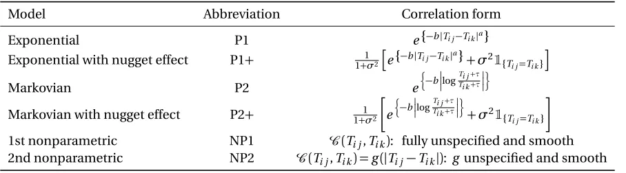
Table 1.1 Correlation models. . . 7

Table 1.2 Comparison of correlation models. . . 13

Table 1.3 MSE(·, P1+) comparison. . . 14

Table 1.4 Estimated parameters for P1+correlation models. . . 15

Table 2.1 Common matrix penalties and proximal maps. . . 31

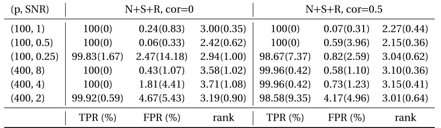
Table 2.2 True positive rate, false positive rate and rank selection result. . . 37

Table 2.3 MSE for signal part. . . 37

Table 2.4 Gene pathway data 10-fold cross-validation result,(n,p,q) = (118, 39, 62). . . 38

Table 2.5 Contaminated gene pathway data (simulated) result,(n,p,q) = (118, 200, 62). . 38

Table 3.1 Scenario I,ρ=0.5, true rank=10. . . 50

Table 3.2 Scenario II,ρ=0.5, true rank=5. . . 50

Table 3.3 Scenario I,ρ=0.5, true rank=10. The three numbers are (Est, Pred, Time). . . 51

Table 3.4 Scenario II,ρ=0.5, true rank=5. The three numbers are (Est, Pred, Time). . . 51

Table 3.5 Simulation results of MSE for penalized matrix regression. . . 52

Table A.1 Correlation matrix for AC . . . 66

Table A.2 Correlation matrix for FL . . . 66

Table A.3 Correlation matrix for HC . . . 67

Table A.4 Scenario I,ρ=0.1, true rank=10. . . 71

Table A.5 Scenario I,ρ=0.9, true rank=10. . . 71

Table A.6 Scenario II,ρ=0.1, true rank=5. . . 72

LIST OF FIGURES

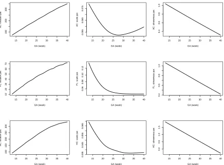
Figure 1.1 Estimated location, scale and skewness parameters as functions of gestational

age for the three fetal growth measurements. . . 8

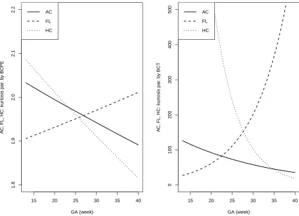
Figure 1.2 Estimated kurtosis parameters as functions of gestational age for the three

fetal growth measurements using BCPE and BCT. . . 9

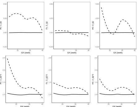
Figure 1.3 Smooth estimates of the first to fourth moments of the constructed Z-scores

for AC (left panel), FL (middle panel) and HC (right panel). . . 10

Figure 1.4 Further comparison of BCCG (solid), BCPE (dashed) and BCT (dotted) on the

fourth moments ofZ-scores. . . 11

Figure 1.5 Smooth estimates of the first and second moments of Z-scores constructed

via BCCG (solid) and SDS (dashed). . . 13

Figure 1.6 Temporal correlations of standardized AC with different correlation models. . 15

Figure 1.7 Observed growth trajectory (linked triangles) and predicted measurements

(dots) given most recent observations of a randomly selected fetus. Dashed line is the population mean. . . 16

Figure 1.8 Longitudinal fetal growth calculator. . . 18

Figure 2.1 Linear and nonlinear regression models based on the same set of pre-selected

covariates for various responses - red: single index model; blue: linear model. In order to compare index model with linear model in the same plot, the coefficient vector for each response is fixed for both models and only the unknown function of the index is considered. . . 23

Figure 2.2 Mean functions for some responses using MSIM model for the gene pathway

data. . . 40

Figure 3.1 Illustration plots for penalized matrix regression. Top left is the true signal

region; top middle is the recovered matrix using a randomly generated initial matrix; top right is the warm-up initial matrix using Frank-Wolfe; Bottom panel contains recovered matrices using warm-up initial matrix with different tuning parameters for penalization. . . 54

Figure A.1 Temporal correlations of standardized FL with different correlation models. . 64

Figure A.2 Temporal correlations of standardized HC with different correlation models. . 65

Figure A.3 Mean functions using MSIM model for the gene pathway data - I. . . 68

Figure A.4 Mean functions using MSIM model for the gene pathway data - II. . . 69

CHAPTER

1

CORRELATION MODELS FOR

MONITORING FETAL GROWTH

1.1

Introduction

During pregnancy, fetal anthropometric measures consisting of head circumference (HC),

abdomi-nal circumference (AC) and femur length (FL) are measured using ultrasound to monitor attained

fetal size at a given gestational age (GA). By comparing measurements to a defined reference or

standard[TW76; Cam80], fetuses with measurements at the extreme ends of the distribution (for

example below the 3rd_{, 5}th_{, or 10}th_{centiles or above the 90}th_{, 95}th_{, or 97}th_{centiles) are identified as}

being at increased risk of a growth disorder, such as intra-uterine growth restriction (IUGR) that

may require further investigation. Growth charts, which conventionally record only cross-sectional

assessment of velocity enables the evaluation of an individual’s growth between any two time points

(rate of growth). These changes observed between two time points may be used to identify those

requiring closer monitoring in the case of great differences between the observed fetal size and what

is expected at a specific time. Notably, fetal growth is rapid in the first and second trimester and

slows towards term. An evaluation of growth velocity ought to consider the correlation of

measure-ments from the same individual. The correlation coefficient is not constant as it is dependent on

the interval between measurements. An estimate of the correlation coefficient is straightforward for

fixed time intervals, but it is clinically useless as, in normal practice, fetuses are seen and measured

at arbitrary time points. For pragmatic reasons, it is impossible to see and measure everyone at fixed

time intervals. Therefore, a flexible model that represents the correlation as a function of time is

required. To the best of our knowledge, correlation models have previously been derived for child

data[Arg08a; And18; Wri94; Col98; Col94]but not for fetal biometry data.

The main aim of this article is therefore, to model the correlation of fetal biometry i.e., HC, AC,

and FL and make available formulae or a tool that can be used to obtain the correlation for each

fetal measure between measurements made at any two time points between 14 and 40 weeks of GA.

We model the correlations using fetal ultrasound data from the INTERGROWTH-21st_{Project Fetal}

Growth Longitudinal Study (FGLS) that were used to construct the international standards for fetal

growth[Pap14; Ohu18]. Further analysis of the cohort demonstrated that the FGLS cohort remained

healthy with adequate growth and motor development up to 2 years of age[Vil18].

1.2

Data

The INTERGROWTH-21st_{Project was a population-based longitudinal study that measured serial}

fetal growth scans every 5±1weeks from recruitment at 9+0- 13+6weeks of gestation until, but not

beyond, 42+0weeks of gestation. The FGLS component of the INTERGROWTH-21stProject is a

unique dataset as it is the largest prospective study to collect data on fetal ultrasound measurements

from optimally healthy pregnant women to date, collecting data in eight geographically diverse

growth scans every 5±1weeks after the initial dating scan, so that the possible ranges after the dating

scan were 14−18, 19−23, 24−28, 29−33, 34−38, and 39−42 weeks of gestation. To ensure all

centres collected high-quality data that were comparable within and between the study sites, all

sonographers and anthropometrists were trained, and all ultrasound measurements were performed

in a standardized manner following strict protocols[Sar13]. All centres adopted uniform methods,

used identical ultrasound equipment in all of the study sites, adopted standardized methodology

to take fetal measurements, and employed locally accredited ultra-sonographers who underwent

standardization training and monitoring.

The analysis was based on the target sample of 4,321 women (20,313 ultrasound scans) who

had pregnancies without major complications and delivered live singletons without congenital

malformations that contributed data for the construction of the INTERGROWTH-21stinternational

fetal growth standards[Pap14], international gestation-specific newborn standards[Vila], gestational

weight gain standards[Lei], and preterm postnatal growth standards[Vil15]. This cohort experienced

very low maternal and perinatal mortality and morbidity rates[Pap14; Vila], confirming that the

participants were at low risk of adverse outcome and therefore contributed to the construction of

the international fetal growth standards. The baseline characteristics of the study cohort across the

eight sites were very similar, which was expected because women were selected from the underlying

low-risk populations using the same clinical and demographic criteria[Pap14; Vilb]. The median

number of ultrasound scans (excluding the dating scan) was 5.0 (mean=4.9, SD=0.8, range from

4 to 7) and 97% of women had 4 scans (mean=5.0, SD=0.6, range from 4 to 7), indicating that

participants adhered well to the protocol. Eighty-five percent of the 20,313 ultrasound scans were

performed within the expected gestational age window of the protocol[Pap14].

The INTERGROWTH-21stProject was approved by the Oxfordshire Research Ethics Committee

“C” (reference: 08/H0606/139), the research ethics committees of the individual participating

in-stitutions, and the corresponding regional health authorities where the project was implemented.

1.3

Statistical Methodology

Consider the longitudinal data{(Ti j,Yi j), 1≤ j ≤mi, 1≤i ≤n}, whereTi j is the gestational age

in weeks for subjecti at the jth visit,Yi j is one of the three ultrasound growth measurements

continuously valued in millimeters atTi j,mi is the number of visits for subjecti, andn is the

number of subjects. Note that the total number of visits can be different for each subject. The goal

is to construct a correlation matrix of the ultrasound measurement at different gestational ages.

Fetuses will not be dichotomized by gender for growth measurement evaluation, and it is also

not the norm as not all populations desire to know fetal sex. Because the marginal distributions of

ultrasound growth measurements may be non-normal, e.g., skewed, a suitable transformation of the

raw growth measurements is first identified and applied to the data to construct a working marginal

reference chart. The raw measurements are then transformed accordingly to provide standardized

deviations (Z-scores). Next the Z-scores are modeled by a Gaussian process with zero mean and

unit variance so that the temporal correlation of the process can be estimated.

1.3.1 Working Models for Marginal Reference Distribution

We consider the LMS transformation[CG92]which could transform non-normal data into normal

data. LetY be a positive random variable and its LMS transformation is given by

Z=

  

 

1 σν

¦€_Y µ

Šν

−1© if ν6=0,

1 σlog

€_Y µ Š

if ν=0.

(1.1)

Hereµ,σ∈R+andν∈Rare location, scale and skewness parameters, respectively. IfZ has a

standard normal distribution, thenY is said to follow the three-parameter Box-Cox Cole-Green

distribution[CG92]denoted by BCCG(µ,σ,ν). A fourth parameter can be added to further model

kurtosis: ifZhas at distribution with degrees of freedomτ∈R+, thenY is said to follow the Box-Cox

t distribution[RS06]denoted by BCT(µ,σ,ν,τ); ifZ has a standard power exponential distribution

denoted by BCPE(µ,σ,ν,τ). Note that BCT(µ,σ,ν,τ= +∞)and BCPE(µ,σ,ν,τ=2)reduce to BCCG(µ,σ,ν).

In practice, ultrasound measurements are often taken at irregular visits, i.e., observed at

gesta-tional ages that differ between subjects. Thus, it may not be feasible to find the proper transformation

at each gestational age separately. Instead, a more practical and statistically efficient approach is

to model the parameters in (1.1) as a smooth function of gestational age. We shall adopt such an

approach and the parameters for BCCG becomeµ(t),ν(t)andσ(t), wheret denotes the gestational

age. The additional parameters in BCT and BCPE are similarly defined. The GAMLSS method[SR07]

can be used to estimate such functions. Under the LMS framework, suppose thatµˆ(t), ˆσ(t), ˆν(t)

are the obtained estimates, then the transformed measurementsZi j can be computed as

Z_{i j}=

  

 

1 ˆ

σ(Ti j)νˆ(Ti j)

§ € _{Yi j}

ˆ µ(Ti j)

Šˆν(Ti j)

−1

ª

if ˆν(T_{i j})6=0,

1 ˆ σ(Ti j)log

€ _{Yi j} ˆ µ(Ti j)

Š

if ˆν(T_{i j}) =0.

(1.2)

Under the BCCG model, marginallyZi j has approximately a standard normal distribution. Under

the BCT or the BCPE models, additional transforms ofZi j are needed to makeZi j normal. For

simplicity, we assume all proper transformations have been taken. Then we modelZi j as a

zero-mean Gaussian process with a constant variance of 1. The Gaussian process is fully identified by

estimating its correlation matrix.

1.3.2 Correlation Models

In this section, we focus on constructing a growth correlation matrix for the Z-scores. We shall

compare several parametric and nonparametric models. The parametric models considered here

are those that have been used for modeling child growth correlation. The exponential model[Dig88]

(denoted by P1) is

cor(Zi j,Zi k) =e{−b|Ti j−Ti k|

a_}

wherea,b∈R+are two unknown parameters that can be interpreted as the order and the rate of

the change in the correlation. This model is commonly used due to its simple form and stationarity,

i.e., the correlation depends only on the distance between two gestational ages. The second model

(denoted by P2), proposed by[Arg08a]for child growth, takes the form

cor(Zi j,Zi k) =e

n

−b

log

Ti j+τ

Ti k+τ

o

,

where τ,b ∈ R+are two unknown parameters. The model is non-stationary, but possesses the

Markovian property. Indeed, via the transformationS_{i j}=log(T_{i j}+τ)andS_{i k}=log(T_{i k}+τ), the corre-lation becomes cor(Z_{i j},Z_{i k}) =ρ|Si j−Si k|_{, where}ρ=_e(−b)_{. Because growth measurements might have} non-ignorable measurement errors, a nugget effect term is usually added to the above correlation

models. The exponential correlation with a nugget effect model (denoted by P1+) takes the form

cor(Zi j,Zi k) = 1 1+σ2

”

e{−b|Ti j−Ti k|a}+σ21 {Ti j=Ti k}

—

,

whereσ2_{is the variance of the measurement error in the Z-scores and1}

{}is the indicator function

which is 1 if the statement inside the bracket is true and 0 otherwise. Similarly, the P2+correlation

model has the form

cor(Zi j,Zi k) = 1 1+σ2

e n −b log

Ti j+τ

Ti k+τ

o

+σ2₁

{Ti j=Ti k}

.

Note that with the nugget term, neither the stationary property nor the Markovian property holds.

Parametric models are simple and easy to interpret, but they can be subject to model

misspecifi-cation. Thus, in addition to the above parametric correlation models, we shall also consider two

nonparametric correlation models. The first one is based on functional data analysis[Yao05], which

Table 1.1Correlation models.

Model Abbreviation Correlation form Exponential P1 e{−b|Ti j−Ti k|a}

Exponential with nugget effect P1+ ₁₊1_σ2

”

e{−b|Ti j−Ti k|a}+σ21

{Ti j=Ti k}

—

Markovian P2 e n

−b

log

Ti j+τ

Ti k+τ

o

Markovian with nugget effect P2+ ₁₊1_σ2

e n

−b

log

Ti j+τ

Ti k+τ

o

+σ2₁

{Ti j=Ti k}

1st nonparametric NP1 C(Ti j,Ti k): fully unspecified and smooth

2nd nonparametric NP2 C(Ti j,Ti k) =g(|Ti j−Ti k|): gunspecified and smooth

a random measurement error term. Specifically, the functional data model is

Zi j=bi(Ti j) +εi j, (1.3)

where b_i(·)is a random and smooth function modeled by a zero-mean Gaussian process with

a smooth covariance functionC(Ti j,Ti k) =Cov{bi(Ti j),bi(Ti k)},{εi1, . . . ,εi mi}are independent

measurement errors with varianceσ2

ε, andbi(·)is independent from the measurement errors.

Such a covariance function does not impose any parametric assumption for modeling correlations

between the repeated observations and is hence very flexible. Since Var(Zi j) =1, the correlation of

the Z-scores at two distinctive time pointsTi j andTi kwithj6=k is automatically given byC(Ti j,Ti k).

Thus, we callC the correlation function and its estimation is described in Section 1.3.3.

The correlation function from the functional data method is in general nonstationary. We shall

also consider a stationary but yet nonparametric correlation by assuming that the correlation

functionC satisfiesC(T_{i j},T_{i k}) =g(|T_{i j}−T_{i k}|), whereg is a smooth but unspecified univariate

function. Note that due to the presence of measurement error in the functional data model, the

overall correlation between the Z-scores is still nonstationary. The estimation ofg is also given in

Section 1.3.3.

15 20 25 30 35 40 100 200 300 GA (week) A

C: location par

.

15 20 25 30 35 40

0.055

0.065

0.075

GA (week)

A

C: scale par

.

15 20 25 30 35 40

0.4 0.6 0.8 1.0 GA (week) A C: skne wness par .

15 20 25 30 35 40

10 20 30 40 50 60 70 GA (week)

FL: location par

.

15 20 25 30 35 40

0.06

0.08

0.10

0.12

GA (week)

FL: scale par

.

15 20 25 30 35 40

0.4 0.6 0.8 1.0 GA (week) FL: skne wness par .

15 20 25 30 35 40

100 150 200 250 300 GA (week)

HC: location par

.

15 20 25 30 35 40

0.035

0.045

0.055

0.065

GA (week)

HC: scale par

.

15 20 25 30 35 40

0.0 0.5 1.0 1.5 GA (week) HC: skne wness par .

Figure 1.1Estimated location, scale and skewness parameters as functions of gestational age for the three fetal growth measurements.

1.3.3 Estimation of the Correlation Models

The parametric correlation models can be easily estimated by maximizing likelihood of theZ-scores

under normality. We now focus on the estimation of the two nonparametric models. Estimation

methods for the functional data model have been well developed in the statistics literature and here

we use the fast covariance estimation method for longitudinal data, developed in[Xia18]. We briefly

describe the method here, which will also be useful for explaining our estimation method for the

second nonparametric model. First, empirical estimates of the correlation function are constructed.

15 20 25 30 35 40

1.8

1.9

2.0

2.1

2.2

GA (week)

A

C

, FL, HC: kur

tosis par

. b

y BCPE

AC

FL

HC

15 20 25 30 35 40

0

100

200

300

400

500

GA (week)

A

C

, FL, HC: kur

tosis par

. b

y BCT

AC

FL

HC

−0.10 −0.05 0.00 0.05 0.10

20 30 40 GA (week) A C: Z_{ij} −0.10 −0.05 0.00 0.05 0.10

20 30 40 GA (week) FL: Z_{ij} −0.10 −0.05 0.00 0.05 0.10

20 30 40 GA (week) HC: Z_{ij} 0.8 0.9 1.0 1.1 1.2

20 30 40

GA (week) A C: Z_{ij}^2 0.8 0.9 1.0 1.1 1.2

20 30 40

GA (week) FL: Z_{ij}^2 0.8 0.9 1.0 1.1 1.2

20 30 40

GA (week) HC: Z_{ij}^2 −0.2 −0.1 0.0 0.1 0.2

20 30 40

GA (week) A C: Z_{ij}^3 −0.2 −0.1 0.0 0.1 0.2

20 30 40

GA (week) FL: Z_{ij}^3 −0.2 −0.1 0.0 0.1 0.2

20 30 40

GA (week) HC: Z_{ij}^3 2.0 2.5 3.0 3.5 4.0

20 30 40

GA (week) A C: Z_{ij}^4 2.0 2.5 3.0 3.5 4.0

20 30 40

GA (week) FL: Z_{ij}^4 2.0 2.5 3.0 3.5 4.0

20 30 40

GA (week)

HC: Z_{ij}^4

2.0 2.5 3.0 3.5 4.0

20 30 40

GA (week)

A

C: Z_{ij}^4

2.0 2.5 3.0 3.5 4.0

20 30 40

GA (week)

FL: Z_{ij}^4

2.0 2.5 3.0 3.5 4.0

20 30 40

GA (week)

HC: Z_{ij}^4

Figure 1.4Further comparison of BCCG (solid), BCPE (dashed) and BCT (dotted) on the fourth moments ofZ-scores.

ri j kis an unbiased estimate ofC(Ti j,Ti k)wheneverj6=k. We will conduct a bivariate smoothing

of the data{(Ti j,Ti k,ri j k), 1≤ j 6=k ≤mi, 1≤i ≤n}to estimate the correlation functionC. We

use bivariateP-splines[EM03], which approximates the bivariate correlation function with

tensor-product B-splines and employs a smoothness penalty to avoid overfit. Moreover, constraints on

spline coefficients are imposed to ensure thatC is symmetric; see[Xia18]for further details. Denote

the corresponding estimate by ˆC(s,t), then we estimate the error varianceσ2

εusing the equality

E(ri j j) = C(Ti j,Ti j) +σ_ε2 for 1≤ j ≤ mi, 1≤ i ≤n. For the second nonparametric model, by

assumption,E(ri j k) =g(|Ti j−Ti k|) +1{j=k}σ2_ε. Thus, we smooth the data{(|Ti j−Ti k|,ri j k), 1≤j6=

k≤mi, 1≤i≤n}to estimate the functiong. Specifically, we use univariateP-splines[EM96], which

approximatesgusing B-spline bases and also controls overfit using a smoothness penalty. Then the

1.4

Results

1.4.1 Marginal Reference Charts

The estimated location, scale and skewness parameters show that a transformation model simpler

than BCCG will be insufficient to fit the data marginally; see Figure 1.1. Our empirical results also

indicate the sufficiency of using BCCG rather than more complicated BCPE or BCT, as Figure 1.2

suggests that the estimated parameter of kurtosis is close to 2 for BCPE model and very large for BCT

model. Figure 1.3 plots the smoothed first to fourth moments of the Z-scores against the gestational

age. Specifically, fork =1, 2, 3, 4, a corresponding nonparametric smooth function is estimated

using the data{Z_{i j}k, 1≤j≤mi, 1≤i≤n}. If the Z-scores are indeed marginally normal, then the

estimated curves should be close to the constant linesy =0, 1, 0, and 3, respectively. Figure 1.3

suggests that the BCCG-transformed Z-scores are marginally normally distributed. A closer look at

the smoothed fourth moments under different models in Figure 1.4 again suggest that BCPE and

BCT are not necessary. We also note that for standardizing the raw measurements, BCCG seems to

be a much better approach than the standard SDS, which presents a systematic biased estimation;

see Figure Figure 1.5.

Consequently, the BCCG model will be applied to construct marginal reference charts.

1.4.2 Correlation Models

We use the BCCG model to fit the marginal distributions of the raw ultrasound measurements

and then convert the transformed measurements into Z-scores. Then different parametric and

nonparametric correlation models are considered and compared via model selection criteria: AIC

and BIC. Both criteria require the degrees of freedom of the model. For parametric correlation

models, it is the number of free parameters. For nonparametric correlation models, the effective

degree of freedom, which evaluates the model complexity of nonparametric smoothers[Rup03],

will be calculated.

−0.25 0.00 0.25 0.50

20 30 40 GA (week)

A

C: Z_{ij}

−0.25 0.00 0.25 0.50

20 30 40 GA (week)

FL: Z_{ij}

−0.25 0.00 0.25 0.50

20 30 40 GA (week)

HC: Z_{ij}

1.0 1.5 2.0 2.5

20 30 40

GA (week)

A

C: Z_{ij}^2

1.0 1.5 2.0 2.5

20 30 40

GA (week)

FL: Z_{ij}^2

1.0 1.5 2.0 2.5

20 30 40

GA (week)

HC: Z_{ij}^2

Figure 1.5Smooth estimates of the first and second moments of Z-scores constructed via BCCG (solid) and SDS (dashed).

Table 1.2Comparison of correlation models.

Models -2log-lik AIC BIC -2log-lik AIC BIC -2log-lik AIC BIC

P1 44656.31 44660.31 44673.01 42790.43 42794.43 42807.13 41999.78 42003.78 42016.48 P1+ 44505.17* 44511.17* 44530.21* 42672.04* 42678.04* 42697.08* 41846.77* 41852.77* 41871.82* P2 45201.95 45205.95 45218.64 43471.66 43475.66 43488.36 42117.83 42121.83 42134.53 P2+ 44540.30 44546.30 44565.34 42708.85 42714.85 42733.89 41943.10 41949.10 41968.15

NP1 44489.71 44509.85 44573.75 42681.81 42697.74 42748.32 41743.67 41783.82 41911.26

NP2 44524.09 44530.36 44550.24 42670.06 42678.54 42705.47 41863.42 41869.44 41888.52

AC FL HC

Note that∗denotes the best parametric model in each column. The bold type denotes the best

Table 1.3MSE(·, P1+) comparison.

Model AC FL HC

NP1 3.93×10−4 _4.46×10−4 _6.33×10−4

NP2 2.25×10−4 6.46×10−5 3.75×10−4

P1 2.87×10−3 1.94×10−3 1.98×10−3

P2+ 9.19×10−4 3.73×10−4 1.08×10−3

P2 1.40×10−2 _1.36×10−2 _2.82×10−3

the P1+model is overall the best model across the three fetal growth measurements. On the one

hand, P1+fits the data best among all parametric models; on the other hand, it has a very simple

form compared to nonparametric methods, and yields the smallest BIC. To quantify the differences

among different correlation models, we use P1+as the reference correlation and evaluate how

the other models differ from P1+. DenoteρP1_{j k}+the correlation coefficient at times(j,k)in P1+

correlation matrix, the mean squared error (MSE) of NP1, for example, to P1+is defined as

MSE(NP1, P1+)= 1

(L−1)(L−2)

X

1≤j<k≤L

€

ρNP1

j k −ρ

P1+

j k

Š2

, (1.4)

whereL=183 is the range of gestational age in days in this study.

Table 1.3 demonstrates an ignorable difference between P1+and NP2, which is as expected

because of the stationarity nature of both models. Furthermore, difference between P1+and NP1 is

also small, suggesting that an exponential correlation model with nugget effect is sufficiently good

for fetal growth measurements. Indeed, the average difference in correlation is only 0.020 for AC,

0.021 for FL and 0.025 for HC. On the other hand, the correlations from the other parametric models

are relatively more divergent from those of P1+compared to the nonparametric models NP1 and

NP2, indicating the superiority of P1+over the other parametric models.

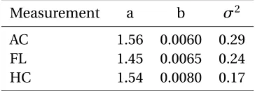
As a result, the estimated parameters for a P1+model are summarized in Table 1.4. For

illustra-tion, we plot the fitted correlation surface on a grid of gestational age by weeks for AC in Figure 1.6.

Table 1.4Estimated parameters for P1+correlation models.

Measurement a b σ2

AC 1.56 0.0060 0.29

FL 1.45 0.0065 0.24

HC 1.54 0.0080 0.17

100 200 300

20 30 40

GA (week)

A

C

20 40 60

20 30 40

GA (week)

FL

100 150 200 250 300 350

20 30 40

GA (week)

HC

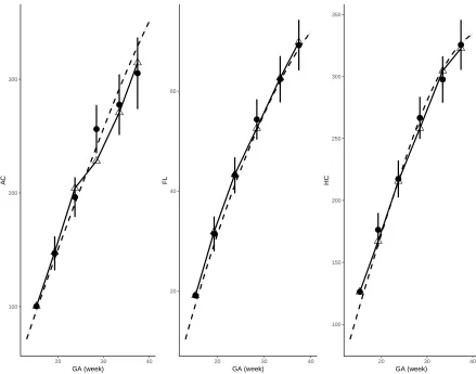
Figure 1.7Observed growth trajectory (linked triangles) and predicted measurements (dots) given most recent observations of a randomly selected fetus. Dashed line is the population mean.

1.5

Case Study: Dynamic Growth Velocity

As an example, we use the result from parametric correlation models to study the growth velocity

of a sample fetus chosen for the purpose of illustration, whose AC, FL and HC are consecutively

measured for 6 times between week 15 and week 38. The observed growth trajectories are shown

as linked triangles in Figure 1.7. Based on each observed measurement atT_j, we also dynamically

predict the measurementTj+1shown as dots, each with a 95% prediction interval. Specifically, each

observed measurement atTj is transformed to Z-score using (1.2). Then, a conditional Z-score

Z_〈Tj+

conditional Z-score is then transformed back to the original measurement given marginal references.

Clinicians might use this approach to compare the observed fetal growth measurements versus its

expected measurements at a certain age to determine if a fetus is growing normally. They can also

calculate and compare velocity increments. We will use the correlations studied in this paper for the

subsequent clinical paper on conditional fetal velocity for use by clinicians.

It is observed that for this randomly sampled fetus, the growth of FL and HC are regular and can

be accurately predicted. For GA, its measurements are higher (still normal) than predicted during

the third visit, but much lower than expected during the fourth visits. This suggests that a closer

monitoring might be needed. The following visits indicate that the GA of the sampled fetus becomes

consistently below the population mean.

To facilitate the usage of the obtained results in practice, a Shiny application is built along with

this paper, where functionalities such as visualization, calculating correlation, prediction and cSDS

are integrated for all the three fetal growth measurements (https://lxiao5.shinyapps.io/shinycalculator/);

see Figure 1.8.

In the meanwhile, correlation tables for fetal growth measurements are provided in appendix.

1.6

Discussion

We have modelled the correlation coefficients of fetal growth for HC, AC, and FL and provided

formulae that can be used to obtain the correlation coefficient for each fetal measure between

measurements made at any two time points between 14 and 40 weeks based on the FGLS data. The

FGLS cohort is the largest prospective study to date to collect data on fetal ultrasound measurements

among optimally healthy pregnant women, used many quality control measures, encompasses

eight geographically diverse populations, was population-based, involved a cohort of women at

low risk of intra-uterine growth restriction and preterm, remained healthy with adequate growth

and motor development up to 2 years of age, hence making it an ideal dataset for characterising the

expected correlation of fetal size measurements[Pap14; Vil18; Sar13; Vil15; Vil13].

lations offered a good fit to the empirical correlation structure. We modelled the correlations in

weekly intervals on the assumption that the correlations were reasonably stable within each week

of gestation. The fitted correlations decreased with increasing time interval as expected. Although

velocity charts could be an important complement to attained size charts[Pap14], they are not often

used clinically. For example, a clinician may be interested to know whether fetal HC at 20 weeks is a

good predictor of that same fetuses HC at 30 weeks. If we know the correlation between these two

time points, then we are able to make inference about what fetal HC might be at 30 weeks given

that we know their fetal HC at 20 weeks. Such predictions can be useful for identifying fetuses that

are faltering in growth i.e., if their observed fetal HC at 30 weeks is significantly less than what was

predicted. This would be indicative of poor growth within that time period that may be require

further investigation or intervention. A limitation of the study was paucity of data and small sample

sizes for some pairs of gestational ages especially in early gestation (first trimester) and at term (40

weeks).

In summary, we have for the first time provided formulae for obtaining correlation coefficients

for fetal biometry using data that was prospectively collected, involved eight countries from diverse

settings, collected using unified protocols, measurement procedures and standardisation, using

high quality data based on the rigorous data quality process that was put in place during the

study period. INTERGROWTH-21stProject is the largest prospective study of fetal growth involving

multiple measurements per fetus that were purposely obtained for the study. These equations for

obtaining corresponding correlation coefficients for any pair of data between 14 and 40 weeks and

consequently the calculation of a velocity Z-score provide a potentially useful tool for clinicians

who wish to monitor the fetal growth and development over time. To facilitate ease of use, a web

application (Shiny application for now) that calculates the expected correlation between any two

time points in the interval 14 to 40 weeks for HC, AC, and FL will be made freely available on the

INTERGROWTH-21st_{website where other applications for fetal, preterm, and newborn size are}

1.7

Acknowledgments

This study was funded by the INTERGROWTH-21st_{grant 49038 from the Bill & Melinda Gates}

Foundation to the University of Oxford; we gratefully acknowledge their support. We would also like

CHAPTER

2

SPARSE SINGLE INDEX MODELS FOR

MULTIVARIATE RESPONSES

2.1

Introduction

Multivariate response linear regression models are commonly used to predict several quantities

simultaneously given a common set of covariates. Consider data{y_i,xi}in=1∈Rq×Rp, a coefficient

matrixB∈Rp×q and uncorrelated random errors{εi}ni=1∈Rq assumingE(εi) =0and Cov(εi) =

σ2_I

q, the model is given by

The model (2.1) may be rewritten more compactly asY=XB+E, whereY= (y₁,· · ·,y_n)T∈Rn×q, X= (x1,· · ·,xn)T∈Rn×pandE= (ε1,· · ·,εn)T∈Rn×q. We assume thatYandXhave been centered so

that intercept is not present in the model.

While univariate regression models can be separately fitted to each response, joint regression

models exploit correlations among responses and hence can be superior in prediction accuracy

[BF97]. Indeed, various methods have been proposed in the literature, such as partial least-squares

regression (PLR), canonical correlation regression (CCR), principal component regression (PCR)

and reduced rank regression (RRR)[Hai98; VR13]. Regularization techniques have been adopted for

multivariate response regression models when predictors or responses reside in high dimensional

spaces. On the one hand, to deal with the challenge of having more predictors than samples, i.e.

p>n, Obozinski et al.[Obo08; Obo10]utilized a block-structured penalty on the coefficient matrix

Bto select covariates that are predictive for all the responses. Peng et al.[Pen10]considered a

combination of penalties that induces both overall sparsity and row sparsity of a matrix. Li et al.

[Li15]proposed models to include arbitrary group structure for the regression coefficient matrix.

On the other hand, whenqis large, low-rank approaches[Yua07; Bun11; Che13; Ma14]are often

adopted by thresholding the singular values ofB. These low-rank models assume the underlying

regression structures have a shared representation for all the responses, and hence have substantially

fewer unknown parameters to estimate, potentially leading to more efficient model estimation.

More parsimonious models can be obtained by enforcing both a variable selection penalty and a

low-rank penalty[Bun12; CH12]to handle high-dimensional models with both largep and largeq.

The problem of multi-task learning[Car98]in the machine learning community presents a similar

problem, and we refer interested readers to Evgeniou & Pontil[EP04], Argyriou et al.[Arg07]and

Argyriou et al.[Arg08b]for some representative work on the multi-task learning.

A key assumption of model (2.1) is the linear relationship between each response and covariates,

which can be seriously violated in practice. Figure 2.1 illustrates the relationship among different

re-sponses and a common set of covariates in a genetic association study, where a joint linear regression

−3 −2 −1 0 1 2

−3

−2

−1

0

1

2

3

Index

At1G06570

−1.5 −0.5 0.5 1.0 1.5

−3

−2

−1

0

1

2

3

Index

A

T5G52570

−2 −1 0 1

−3

−2

−1

0

1

2

3

Index

A

T5G24150

Figure 2.1Linear and nonlinear regression models based on the same set of pre-selected covariates for various responses - red: single index model; blue: linear model. In order to compare index model with linear model in the same plot, the coefficient vector for each response is fixed for both models and only the unknown function of the index is considered.

potential nonlinear relations. Because of the curse of dimensionality, a fully nonparametric

regres-sion approach is often undesired. To address the dimenregres-sion problem, Yuan et al.[Yua07]proposed

additive models for each response, where each additive component is a nonparametric univariate

function of a covariate. An alternative approach is the single index model (SIM), in which each

response is modeled as a nonparametric function of an index that is a linear combination of the

covariates. For univariate response (q=1), SIM, as well as its various forms, such as partially linear

SIM and generalized SIM, were extensively studied by Härdle & Stoker[HS89], Ichimura[Ich93],

Carroll et al.[Car97], Hristache et al.[Hri01], Liang et al.[Lia10]and Wang et al.[Wan10]using kernel

methods, and by Yu & Ruppert[YR02]and Wang & Yang[WY09]using splines. For spline-based

methods, recent studies of Kong & Xia[KX07]and Foster et al.[Fos13]considered the problem of

variable selection for SIM.

To tackle both potential nonlinearity in multivariate response regression and challenges in

the response vectory_iis linked to covariatesxiand coefficient matrixBthroughqunknown and unspecified link functionsF ={f1, . . . ,fq}such that

y_i = f₁(xT_iB_·1),· · ·,fq(xT_i B·q) T

+εi. (2.2)

In (2.2),B_·j ∈Rp is the jth column ofBand is the coefficient vector corresponding to the jth

response yi j inyi = (yi1,· · ·,yi q)T for all i = 1,· · ·,n. For model identifiability we assume that

kB_·jk22=1, and without loss of generality letb1j, the first element ofB·j, be nonnegative. Such an

assumption is commonly used in single index models[Ich93]. Moreover, we shall assume thatBhas

sparse structures that induces information sharing among multivariate responses. For example,

we assume that the non-zero rows ofBare sparse, or the vector of singular values ofBare sparse,

or both are sparse. We will impose these sparsity structures via corresponding penalty functions,

as shall be shown later in this paper. The recovery of the sparsity structures inBand the form of

the link functions could thus provide insights on how the covariates are related to multivariate

responses. However, to the best of our knowledge, the problem of MSIM with multiple penalties has

not been addressed in the literature. Thus, the main contribution of this paper is a computational

framework for jointly estimating the unknown smooth link functionsF and coefficient matrixB

under a general collection of structure-inducing assumptions. At a high level we employ a classic

alternating strategy for estimatingF conditioned onBand vice versa. The former problem can be

solved using existing nonparametric methods. The latter, however, requires a new approach based

on the alternating direction method of multipliers (ADMM).

The rest of this paper introduces our framework in the following stages. In Section 2.2, we

describe the main model framework and discuss various sparsity-inducing penalties for MSIM.

In Section 2.3, we detail a new alternating two-step iterative algorithm for regularized MSIM. In

Section 2.4, we discuss how to choose tuning parameters for the model. In Section 2.5 and Section 2.6,

we demonstrate the effectiveness of our model through simulation studies and an application in a

2.2

Regularized MSIM

We first introduce notation. Bold upper-case letters (e.g.B) denote matrices, bold lower-case letters

or upper-case letters with dot notation (e.g.b,B_·j orBk·) denote vectors and lower-case letters

denote scalars (e.g.b). In particular, for any matrixB, we useB_·j andBk·to denote the jth column

andkth row ofB, respectively. We usek·k2to denote the Euclidean norm of a vector andk·kFto

denote the Frobenius norm of a matrix.

To fit our proposed regularized MSIM (2.2), we consider the following optimization problem:

minimize F,B

¨

LF(B) + h

X

l=1

Rl,λl(B)

«

(2.3)

subject to identifiability constraintskB_·jk22=1 andb1j ≥0 for j =1, . . . ,q. In (2.3),LF is a loss

function depending on theqlink functions andRl,λl is a regularizer each depending on a tuning

parameterλl. Treatingfj as an elementwise function if its argument is a vector and noticing that

Y_·j−f_j(XB_·j) 2 2=

Pn

i=1

yi j−fj(xTiB·j)

2

, we shall use least-squares loss

LF(B) = 1 2n

q

X

j=1

Y_·j−f_j(XB_·j) 2 2.

Thejth column ofY, i.e.Y_·j = (y1j,· · ·,yn j)T, corresponds to thejth response.

The regularizerRl,λl enforces sparsity onB. We use multiple sparsity-inducing penalties to

recover a parsimonious and sparse coefficient matrixB. Below we review some popular matrix

penalties.

• Column penalty

By treating each column ofBas a block, penalizing column vectors inByieldsq sparse

SIMs under the least-squares loss. For a fixed indexj, problem (2.3) reduces to minimizing

Lfj(B·j)+Rλ(B·j), whereLfj(B·j) =

1

2nkY·j−fj(XB·j)k22. This is a generic model to study variable

lasso[Zou06], SCAD[FL01], MC+ [Zha10]and so on have been studied under the assumption

thatfj is a linear function and consequently some have been applied to the SIM by Carroll

et al.[Car97], Liang et al.[Lia10], Peng & Huang[PH11]and Foster et al.[Fos13]. Our model

includes sparse SIM as a special case and the algorithm proposed to solve (2.3) is directly

applicable for this simpler model.

• Row penalty

The row penalty is a group lasso type penalty that penalizes each row ofBas a group. The

implication of the row penalty is that it identifies covariates that are active for predicting all

qresponses simultaneously in a joint model. Take theL_2,1norm regularization for example;

it is equivalent to a group lasso penaltyRλ(B) =λPpk=1kBk·k2[YL06]. The tuning parameter

λcontrols the amount of shrinkage to each row. Whenq =1, this penalty reduces to the

standard lasso penalty for SIM.

• Rank penalty

It is often useful to assume that the coefficient matrixBhas low-rank. To induce the recovery

of a low-rankB, we may useRλ(B) =λrank(B)or its tightest convex relaxationRλ(B) =λkBk∗

that penalizes the nuclear norm ofB. Extensions of this line of research include, for example,

Chen et al.[Che13]and Josse & Sardy[JS16]. An alternative way to achieve the recovery of a

low-rankBis to directly fix the rank of the coefficient matrix; see, e.g. Bunea et al.[Bun12]and

Chen & Huang[CH12].

In addition to these penalties, we can also penalize individual elements inB, or any group

of elements properly defined. In principle, the form of the penalty is based on the structure of

the coefficient matrix that one wishes to recover. Our proposed model estimation is general and

accommodates different types and combinations of penalties, but the computational challenge also

increases as we increase the number of structure-inducing penalties. The next section introduces a

flexible and general framework based on alternating minimization and the ADMM algorithm for

marriage of the row penalty and the rank penalty will be the extensively studied under MSIM in

later sections.

2.3

Estimation

Simultaneously estimating a collection ofq unknown smooth functionsF ={f1, . . . ,fq}and the

index coefficient matrixBis computationally challenging. Estimating the collection of functionsF

givenB, and vice versa estimatingBgivenF, in contrast is computationally more straightforward

and consequently a commonly used strategy in fitting single index models[WY09; Fos13]. Thus, we

adopt the following two-step iterative approach.

Step 1: Given the index coefficient matrixB, we estimate each response fj ∈ F via univariate

smoothing; see Section 2.3.1.

Step 2: GivenF, we estimateBvia the proposed optimization algorithm in Section 2.3.2.

To obtain an initial estimate ofB, we fitqunivariate ridge regressions separately.

2.3.1 Step 1: Estimating_F

Given the index coefficient matrixB, we fit each unknown and unspecified functionfj using

penal-ized splines[EM96]. Letui j =xTi B·j be the index for the jth response, thenyi j=fj(ui j) +εi j. The

penalized splines approximatef_j(t)by a linear combination of B-splines, i.e.

fj(t) = m

X

k=1

θk jφk j(t), (2.4)

where{φ1j(t), . . . ,φm j(t)}is a set ofmcubic B-spline basis functions constructed from

equally-spaced knots defined in the range ofu_{i j} andθ_{k j} are the associated coefficients to be estimated. To

simplify notation, we use the same number of B-spline basis functions for all responses. Note that

the knots depend on the range of the indices and hence are response specific. Moreover, they could

are iteratively updated. In practice we use 10 basis functions to reduce the approximation bias and

enforce a smoothness penalty on the estimate to control over-fitting. Specifically, we estimate the

coefficientsΘ_·j= (θ1j, . . . ,θm j)Tby minimizing

Qγj(Θ·j) = 1 2n

n

X

i=1

¨

yi j− m

X

k=1

θk jφk(ui j)

«2

+γjΘT_·jDΘ·j, (2.5)

whereDis a second-order difference penalty matrix[EM96]andγj is a smoothing parameter that

balances model fit and model complexity. The optimization problem is a least-squares problem

and to quickly and automatically selectγj, we use generalized cross-validation (GCV)[Rup02]for

each response.

2.3.2 Step 2: Estimating B

Even withF fixed, estimatingBis not straightforward when multiple non-smooth sparsity inducing

penalties are involved. To address this challenge, we introduce a collection of dummy variablesC =

{C₀,C₁,· · ·,Ch}, one for each of theh+1 penalty terms. GivenF, the following equality constrained problem is equivalent to problem (2.3) after variable splitting:

minimizeLF(B) +

h

X

l=1

Rl,λl(Cl) +

q

X

j=1

ιS C0,·j

subject toB=C0=C1=· · ·=Ch,

(2.6)

whereι_S is the indicator function of the identifiability constraint setSand is given by

ιS(c) =

  

 

0 ifkck2=1 andc1≥0,

+∞ otherwise.

With the help of dummy variablesC, the optimization problem in (2.6) can be iteratively solved

using the classic alternating direction method of multipliers (ADMM) algorithm[GM76; GLT89]. In

problems[Boy11]. The algorithm for (2.6) admits a simple iterative block updates for the matricesB

andCl’s that involve minimizing the augmented Lagrangian function of (2.6). Let〈A,B〉=tr(ATB)

denote the inner product between the matricesAandB, then the augmented Lagrangian function

of (2.6) is

Lρ(B,C,M) = LF(B) + h

X

l=1

Rl,λl(Cl) +

q

X

j=1

ιS C0,·j

+Q(B,C,M)

where

Q(B,C,M) =

h

X

l=0

Ql(B,Cl,Ml) = h

X

l=0

〈Ml,Cl−B〉+

ρ

2kCl−Bk

2 F

,

M={M0,· · ·,Mh}are Lagrange multiplier matrices, andρis a positive tuning parameter. We will

discuss the choice ofρin next section.

At thekth iteration of the algorithm, minimization of the augmented Lagrangian is illustrated

by the following steps:

• Update 1:B(k+1)_{=arg min}

B LF(

B) +Q B,C(k)_,M(k)

• Update 2:C(_lk+1)=        arg min C0 Q0 €

B(k+1),C0,M(0k) Š

+Pq

j=1ιS C0,·j

ifl=0

arg min

Cl

Ql

€

B(k+1),Cl,M(

k)

l

Š

+Rl,λl(Cl) ifl>0

• Update 3:M(_lk+1)=M(_lk)+ρ€C(_lk+1)−B(k+1)Š

Update 1: B

Due to the sum-of-squares structure of the Frobenius norm, defineg_j(k)(B_·j) =21nkY·j−fj(XB·j)k22+ Ph

l=0

§ ¬

M_l(k_,·)_j,C_l(k_,·)_j−B_·j

¶ +ρ₂

C

(k)

l,·j−B·j

2 2 ª

, thenBcan be updated column by column through

B(_·k_j+1) = arg min

B·j

However, there is no explicit solution to optimize a generalgj, thus we propose to inexactly minimize

(2.7) using a first-order or second-order method. With the spline representation (2.4), f_j0and f_j00

can be estimated together to formulate the gradient∇gj and the Hessian matrix∇2gj (see the

supplemental materials). Thus, for an iterative optimization algorithm nested in the(k+1)th iteration

of the ADMM algorithm, we setB_·(k_j+1,1)=B(_·k_j)as the initial value and iterate by the formula

B(_·jk+1,m+1) = B(_·k_j+1,m)−tm∇gj(k)

€

B(_·k_j+1,m)Š, (2.8)

wheret_m is a step size that can potentially depend on the current inner iteration indexm.

Symboli-cally, the desired final result isB(_·k_j+1)=lim_m→∞B(_·k_j+1,m), but in practice we stop when the relative change of two consecutive iterations falls within a pre-specified threshold. To achieve a balance

between the convenience and speed of the inner-loop and the convergence rate, we recommend

using a quasi-Newton type algorithm (e.g. BFGS), where an approximate Hessian matrix∇Ö2g_j is

updated through a recursion requiring only the information of first-order derivative∇gj andfj0.

Then we replacetm by∇Ö2g_j

−1

in (2.8).

Update 2: C0

Similar to the column-wise update toB, after some simple manipulations, we can see the subproblem

in this step is to minimizeιS C0,·j

+ρ2

C0,·j−B

(k+1)

·j +ρ−1M

(k)

0,·j

2

2. The solution is

C(_0,k_·+_j1) = PS

€

B(_·k_j+1)−ρ−1M(_0,k_·)_jŠ, (2.9)

wherePS(·)is the Euclidean projection of a vector onto the surface of unit-ball with the first element

being nonnegative.

Update 2: Cl

Without loss of generality, we ignore the subscriptl and consider one penalty at a time. Then the

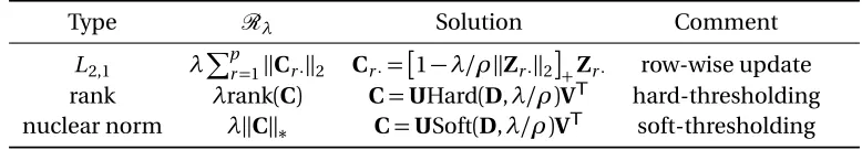
Table 2.1Common matrix penalties and proximal maps.

Type Rλ Solution Comment

L_2,1 λPp

r=1kCr·k2 Cr·=

1−λ/ρkZr·k2

+Zr· row-wise update

rank λrank(C) C=UHard(D,λ/ρ)VT hard-thresholding

nuclear norm λkCk∗ C=USoft(D,λ/ρ)VT soft-thresholding

then have

C(k+1) = arg min

C Rλ

(C) +ρ

2kC−B

(k+1)_+ρ−1_M(k)

k2F. (2.10)

The subproblem of (2.10) is known as the proximal map and for many useful regularization penalties,

there exists explicit solutions[CW05; PB14; Pol15]. We illustrate this result by first defining a new

response matrixZ(k)=B(k+1)−ρ−1M(k). UnderL2,1penalty, for instance, the explicit solution is to

updateCrow by row through

C(_rk_·+1) = 1−λ/ρkZ(_rk_·)k2

+Z(

k)

r· ,

wherer =1,· · ·,pand[u]₊=max{0,u}denotes the positive part of the scalaru. Moreover, Table 2.1

summarizes some common matrix penalties mentioned in Section 2.2 and their corresponding

proximal maps. Note that after singular value decomposition of the new response matrix SVD(Z) =

UDVT, Hard(D,λ/ρ)is the element-wise hard thresholding of the diagonal matrixDwith tuning

parameterλ/ρand similarly Soft(D,λ/ρ). Also note that with penalties in Table 2.1, the updates are

all non-iterative.

Another useful type of rank penalization is to restrict the minimizer to have exactly rankr using

the indicator function

ιr(C) =

  

 

0 if rank(C) =r,

as the penalty function. This is a fixed rank approach, which is similar to but computationally

cheaper than using a tuning paramterλto penalize the rank because differentλ’s may result in a

same matrix having a particular rank. For the simplicity of narration, we treatr andλequally in

tuning parameter searching.

It is obvious that by using this block updating approach, we can conveniently recover a coefficient

matrix that has various structures at the same time by switching among different penalties.

2.3.3 Marginal Screening and Identifiability

When applying theL2,1norm penalty on the coefficient matrixBto conduct variable selection, it is

possible that a large tuning parameterλshrinks all rows inBto zero. This problem also exists for

SIM, and will apparently violate the identifiability constraints. A possible solution would be to leave

a certain row ofB, denoted byBK·, unpenalized and keep the sign to be positive for each element in

this row. In this case, there is always one active covariate for all responses. The choice of theKth

row, however, is not trivial. Motivated by the nonparametric variable screening technique[Fan11],

we propose finding the particular covariate having a combined largest effect for all responses.

Consider univariate simple nonlinear regression for the thejth response andkth covariateyi j=

µk j(xi k) +εi k j, whereεi k j are i.i.d. errors. Thus, we can chooseK by

K = arg min

k q

X

j=1

n

X

i=1

{yi j−µˆk j(xi k)}2.

ˆ

µk j can be obtained by any standard univariate smoothing technique. In our application, we apply

the penalized spline smoother with tuning parameter selected by GCV.

2.3.4 Algorithm, Computation Complexity and Convergence

The above discussion leads to Algorithm 1 for regularized MSIM. Note that in practice we will

termi-nate the algorithm after finitely many iterations. At termination each dummy variable will posses