ABSTRACT
FERRACO SCOLFORO, HENRIQUE. Development of a Modeling Framework for Clonal Eucalypt Plantations Subject to Different Environmental Conditions in Brazil. (Under the direction of Dr. Joseph Roise).
Development of a Modeling Framework for Clonal Eucalypt Plantations Subject to Different Environmental Conditions in Brazil
by
Henrique Ferraco Scolforo
A dissertation submitted to the Graduate Faculty of North Carolina State University
in partial fulfillment of the requirements for the degree of
Doctor of Philosophy
Forestry and Environmental Resources
Raleigh, North Carolina 2018
APPROVED BY:
_______________________________ _______________________________ Dr. Joseph Roise Dr. John Paul McTague
Committee Chair
_______________________________ _______________________________ Dr. Harold Burkhart Dr. Jose Luiz Stape
External Member
ii DEDICATION
iii BIOGRAPHY
iv ACKNOWLEDGMENTS
I wish to express my most sincere appreciation to my committee members for their guidance and support through this process. To Dr John Paul McTague that changed my perceptions regarding sampling, mensuration and advanced forest biometrics, spent many days sharing his knowledge, techniques and valuable ideas with me, for all his enthusiasm to teach me several biometrics and stats topics and really pushed me to be a better professional. To Dr Stape for giving me a unique opportunity to come to USA, for introducing me to a new and great world by teaching me how important and crucial is to address the factors that governs forest production, for sharing his knowledge and valuable ideas in ecophysiology with me, for facilitating my funding and for making me part of the TECHS project. To Dr Roise that became my major professor in 2015, shared his vast experience in forest planning with me and gave me the opportunity of keep working on the same research that I was working on. To Dr Burkhart for his enthusiasm, for all the unique and valuable ideas shared in advanced forest biometrics and forest management, and for all his support and assistance in the dissertation writing and analysis. To Dr McCarter for all the knowledge that was shared about programming in a variety of languages. To Dr Dickey for all the hints and conversations about statistics as an effective tool in forestry, especially the ones in mixed modeling and data mining.
v I wish to express my sincere appreciation to CNPq – Conselho Nacional de Desenvolvimento Cientifico e Tecnologico do Ministerio da Ciencia e Tecnologia of Brazil government – for the unique scholarship provided to develop this research (249979/2013-6).
I wish to express my sincere appreciation to NCSU, with special thanks to Dr John Welker (for the valuable ideas and hints shared in forest planning), to Dr Rachel Cook, to Dr Barry Goldfarb and to Dr Bullock. Also to Dr Montes (for the valuable ideas shared in precision silviculture and modeling) and to Dr Weiskittel (for the valuable ideas shared in modeling).
I wish to express my most sincere appreciation to my wonderful wife (Paula) for her love, care and support throughout this process. Without her, I would not be able to make this degree.
I wish to express my sincere appreciation to my beloved parents (Jose Scolforo and Sandra), to my beloved sister (Roberta) and to my beloved relatives (well represented by Jair and Isaura Ferraco; Jose and Aurora Scolforo). Without this amazing family, I would not be the person that I am today. I wish to express my sincere appreciation to my great friends: Adriana McTague, Patsie Welker, Jody, Sharon, Kevin, Vitor, Kathryn, Brazilian Bruno, Maria, Portuguese Bruno, Adriana, Rafa, Eduardo Ruas, Morgan, David, Mai Duong, Lucas, Thiza, Pedro, Marcel, Omar, Samuel, Ronan, Venicios, Matheus and Fernando.
vi TABLE OF CONTENTS
LIST OF TABLES ……….……...xi
LIST OF FIGURES………....……..xiv
CHAPTER 1: INTRODUCTION ... 1
REFERENCES ... 5
CHAPTER 2: GENERALIZED STEM TAPER AND TREE VOLUME EQUATIONS APPLIED TO EUCALYPTUS OF VARYING GENETICS IN BRAZIL ... 6
Abstract ... 6
1. Introduction ... 7
2. Material and methods ... 10
2.1. Database ... 10
2.2. Tree volume and stem taper equations ... 13
2.2.1. Tested climatic variables ... 14
2.2.2. Penalized Mixed Spline (PMS) ... 14
2.2.3. Total and merchantable volume models ... 17
2.3. Goodness of fit ... 19
3. Results ... 20
3.1. Stem taper predictions over different clones ... 20
3.2. Total tree volume prediction based on the generalized PMS taper functions and diameter inside bark equations ... 24
3.3. Total tree volume prediction over different clones by the Schumacher and Hall (1933) equation ... 27
3.4. Volume ratio predictions and comparison of these equations with the generalized PMS taper model and diameter inside bark equations ... 30
4. Discussion... 34
5. Conclusions ... 37
REFERENCES ... 39
CHAPTER 3: YIELD PATTERN OF EUCALYPT CLONES ACROSS BRAZIL: AN APPROACH TO CLONAL GROUPING ... 42
Abstract ... 42
1. Introduction ... 44
2. Material and methods ... 46
2.1. Characterization of the sites and database ... 46
2.2. Standardized volume yields of the clones ... 49
vii
3. Results ... 56
3.1. Fitted equation for standardizing the volume yields of the clones ... 56
3.2. Identifying clones with similar yield pattern across Brazil – clonal grouping... 58
4. Discussion... 64
5. Conclusions ... 67
REFERENCES ... 68
CHAPTER 4: COMPATIBLE SET OF PREDICTION AND PROJECTION DOMINANT HEIGHT EQUATIONS FOR CLONAL EUCALYPT PLANTATIONS IN BRAZIL: A MODELING APPROACH EXPANDED AND REFINED BY ENVIRONMENTAL VARIABLES ... 71
Abstract ... 71
1. Introduction ... 73
2. Material and methods ... 75
2.1. Study area and database ... 75
2.2. Dominant height growth modeling ... 80
2.3. Parameters expanded and refined by environmental variables ... 83
2.4. Assessing and validating the modeling approaches ... 84
3. Results ... 85
3.1. Selection of the best compatible set of prediction and projection dominant height growth equations for Brazil ... 85
3.2. Expanding and refining the asymptote parameter of the compatible prediction/projection Chapman-Richards growth equations with environmental variables ... 89
3.3. Practical purposes of the developed modeling approach with the inclusion of SWD ... 97
3.4. Current productive potential of clonal eucalypt plantations in Brazil ... 102
4. Discussion... 104
5. Conclusions ... 107
REFERENCES ... 109
CHAPTER 5: MODELING WHOLE-STAND SURVIVAL IN CLONAL EUCALYPT STANDS IN BRAZIL AS A FUNCTION OF WATER AVAILABILITY ... 112
Abstract ... 112
1. Introduction ... 113
2. Material and methods ... 115
2.1. Sites and database... 115
viii 2.2.1. Approach 1: Direct estimation of whole-stand survival through the use of
ADA ... 120
2.2.2. Approach 2: Two-step approach ... 122
2.2.2.1. Logistic model... 122
2.2.2.2. Estimation of whole-stand survival through the use of ADA... 123
2.2.2.3. Deterministic approach based on decision theory ... 124
2.2.3. Modeling survival as a function of cumulative soil water deficit ... 124
2.3. Validation of whole-stand survival modeling approaches... 126
3. Results ... 127
3.1. Selection of the best difference model for the direct projection of whole-stand survival ... 127
3.2. Assessment of the two-step approach for the projection of whole-stand survival .... 128
3.2.1. Selection of the difference model for estimation of whole-stand survival ... 128
3.2.2. Assessment of the logistic model for predicting the probability of no mortality occurrence ... 129
3.2.3. Assessment of the deterministic approach based on decision theory for projecting whole-stand survival ... 130
3.3. Modeling whole-stand survival as a function of cumulative soil water deficit... 130
3.4. Assessing SWD scenarios and how these affect whole-stand survival in clonal eucalypt stands in Brazil ... 133
4. Discussion... 135
5. Conclusions ... 138
REFERENCES ... 139
CHAPTER 6: STAND-LEVEL GROWTH AND YIELD SYSTEM FOR CLONAL EUCALYPT PLANTATIONS IN BRAZIL: A SYSTEM THAT ACCOUNTS FOR WATER AVAILABILITY ... 142
Abstract ... 142
1. Introduction ... 144
2. Material and methods ... 146
2.1. Study area and database ... 146
2.2. Climate information ... 149
2.3. Stand-level models ... 151
2.3.1. Basal area modeling ... 152
2.3.2. Volume modeling ... 155
2.4. Validation of the growth and yield system that accounts for water availability ... 156
ix
2.4.2. Assessing basal area accuracy ... 159
2.4.3. Comparison between a typical growth and yield system and growth and yield system that accounts for water availability ... 159
3. Results ... 160
3.1. Selection of the equation that simultaneously predicts and projects basal area ... 160
3.2. Comparison between a typical growth and yield system and growth and yield system that accounts for water availability ... 169
3.3. Current eucalyptus productivity in Brazil... 173
4. Discussion... 176
5. Conclusions ... 178
REFERENCES ... 180
CHAPTER 7: EUCALYPTUS GROWTH AND YIELD SYSTEM: LINKING INDIVIDUAL-TREE AND STAND-LEVEL GROWTH MODELS IN CLONAL EUCALYPT PLANTATIONS IN BRAZIL ... 182
Abstract ... 182
1. Introduction ... 184
2. Material and methods ... 186
2.1. Study area ... 186
2.2. Database ... 188
2.3. Individual-tree modeling ... 191
2.3.1. Diameter percentiles ... 192
2.3.2. Mortality ... 194
2.3.3. Generalized height-diameter equation ... 195
2.4. Linking individual-tree and stand-level growth models ... 195
2.4.1. For projection purposes: applied to inventory plots for growth updates and forecasts ... 198
2.4.1.1. Number of trees per DBH class estimated from the individual-tree mortality equation and survival estimates based on whole-stand survival ... 198
2.4.1.2. Individual-tree growth implied by the Weibull distribution ... 199
2.4.2. For prediction purposes: applied to areas without inventory records ... 202
2.4.3. Volume estimates ... 203
2.5. Validation ... 204
2.5.1. Validation of the individual-tree models ... 205
2.5.2. Validation of the eucalyptus growth and yield system ... 205
x
3.1. Diameter percentile modeling... 206
3.2. Individual-tree mortality modeling ... 210
3.3. Individual-tree height modeling ... 211
3.4. Assessment of the G & Y system for long-term projections based on young eucalypt stands ... 213
3.5. Assessment of the G & Y system for long-term predictions ... 219
4. Discussion... 220
5. Conclusions ... 223
REFERENCES ... 224
CHAPTER 8: OVERALL CONCLUSIONS... 227
APPENDICES ... 230
Appendix A. Fitted coefficients with their standard errors of the generalized PMS equation [Equation (1)]. ... 231
Appendix B. Fitted coefficients with their standard errors of the generalized dib equation [Equation (3)]. ... 232
Appendix C. Fitted coefficients with their standard errors of the generalized total volume equation [Equation (4)]. ... 233
xi LIST OF TABLES
CHAPTER 2: GENERALIZED STEM TAPER AND TREE VOLUME EQUATIONS
APPLIED TO EUCALYPTUS OF VARYING GENETICS IN BRAZIL ... 6 Table 1. Descriptive statistics for each clone of the eucalyptus plantations. ... 12 Table 2. Climate description of the TECHS sites. ... 13 Table 3. Fitted coefficients with their standard errors (SE) of Eqs 1-2, and goodness of fit
indicators (logLik, AIC, BIC, T, MAE, RMSE and EF). ... 21 Table 4. Fitted coefficients with their standard errors (SE) of Eq. (3), and goodness of fit
indicators (logLik, AIC, BIC, T, MAE, RMSE and EF) to predict dib at any stem height... 23 Table 5. Goodness of fit indicators (T, MAE, RMSE and EF) to predict total tree volume
outside bark (Traditional, WD, P-PET, Tavg) and inside bark volume (vib), in m3. ... 25
Table 6. Fitted coefficients with their standard errors (SE), and goodness of fit indicators for Equations 4-5 (logLik, AIC, BIC, T, MAE, RMSE and EF). ... 28 Table 7. Fitted coefficients with their standard errors (SE), and goodness of fit indicators for
Equations 6-7 (logLik, AIC, BIC, T, MAE, RMSE and EF). ... 31 Table 8. Performance (T, MAE and RMSE) of the top diameter volume ratio and PMS
equations along different top diameters (cm). ... 34 CHAPTER 3: YIELD PATTERN OF EUCALYPT CLONES ACROSS BRAZIL: AN
APPROACH TO CLONAL GROUPING ... 42 Table 1. TECHS sites and their average key environmental attributes between the period of
2012-2017. ... 49 Table 2. Fitted coefficients for the fixed β parameters of Eq. 2 and their associated standard
errors (SE, m3.ha-1) of the fitted polynomial... 56
Table 3. Average volume yield (𝑉) in m3.ha-1, mean annual water deficit index (𝑊𝐷𝐼) in
mm.year-1, fitted linear regressions and the general groups to which each clone
belongs. ... 59 Table 4. Fitted coefficients of Eq. 11 and their associated standard errors (SE, m3.ha-1) of the
fitted linear mixed effect model for the group: high productivity and sensitive to
climate variation... 62 Table 5. Fitted coefficients of Eq. 11 and their associated standard errors (SE, m3.ha-1) of the
fitted linear mixed effect model for the group: low productivity and sensitive to
xii CHAPTER 4: COMPATIBLE SET OF PREDICTION AND PROJECTION DOMINANT HEIGHT EQUATIONS FOR CLONAL EUCALYPT PLANTATIONS IN BRAZIL: A MODELING APPROACH EXPANDED AND REFINED BY ENVIRONMENTAL
VARIABLES ... 71 Table 1. Overall descriptive statistics of dominant height (H) under regular plots and
rainfall exclusion regime plots. ... 77 Table 2. TECHS sites and the recorded weather attributes in the measurement periods. ... 80 Table 3. Tested base models and dynamic models to simultaneously predict and project
dominant height in clonal eucalypt plantations. ... 82 Table 4. Fitted coefficients of the compatible set of prediction and projection dominant
height growth equations and their fitting statistics (AIC and BIC). ... 86 Table 5. Validation statistics of the fitted compatible set of prediction and projection
dominant height growth equations. ... 87 Table 6. Fitted coefficients of the fitted compatible set of prediction and projection dominant
height growth equations with the inclusion of environmental variables and the
associated fit statistics (AIC and BIC). ... 90 Table 7. Validation statistics of the fitted compatible set of prediction and projection
dominant height growth equations with the inclusion of environmental variables. ... 91 Table 8. Validation statistics of the fitted compatible set of prediction and projection
dominant height growth equations (M2_2 and M2_2 with the inclusion of SWD) for the rainfall exclusion plots. ... 97 CHAPTER 5: MODELING WHOLE-STAND SURVIVAL IN CLONAL EUCALYPT
STANDS IN BRAZIL AS A FUNCTION OF WATER AVAILABILITY ... 112 Table 1. TECHS sites and the recorded attributes (annual soil water deficit - SWD,
site index - S, surviving TPH - N, planted TPH – Np). ... 118
Table 2. Tested whole-stand survival equations. ... 122 Table 3. Fitting (AIC and BIC) and validation (Bias, MAE, and RMSE for TPH (N2), and
EF) statistics of the difference equations for the direct projection of whole-stand
survival. ... 127 Table 4. Fitting (AIC and BIC) and validation (Bias, MAE, and RMSE for TPH (N2), and
EF) statistics of the difference equations for the projection of whole-stand survival. 129 Table 5. Fitting (AIC and BIC) and validation (Bias, MAE, and RMSE for TPH (N2), and
EF) statistics of the difference equation (Eq. (10)) for the direct projection of
xiii CHAPTER 6: STAND-LEVEL GROWTH AND YIELD SYSTEM FOR CLONAL
EUCALYPT PLANTATIONS IN BRAZIL: A SYSTEM THAT ACCOUNTS FOR
WATER AVAILABILITY ... 142 Table 1. Overall descriptive statistics of basal area and stand-level volume under regular
plots and rainfall exclusion regime plots. ... 148 Table 2. TECHS sites and the recorded weather attributes in the measurement periods. ... 151 Table 3. Fixed effects fitted coefficients of the compatible set of prediction and projection
basal area equations and their fitting statistics (AIC and BIC). ... 161 Table 4. Validation statistics (T - m2.ha-1, MAE - m2.ha-1, RMSE - m2.ha-1, and EF) of the
fitted compatible set of prediction and projection basal area equations with and
without the inclusion of soil water deficit... 162 Table 5. Fixed fitted coefficients of the volume equation and the fitting statistics
(AIC and BIC)... 169 Table 6. Validation statistics (T – m3.ha-1, MAE – m3.ha-1, RMSE – m3.ha-1, and EF) for
stand-level volume estimates. Validation was conducted using exclusively the
rainfall exclusion plots. ... 170 CHAPTER 7: EUCALYPTUS GROWTH AND YIELD SYSTEM: LINKING
INDIVIDUAL-TREE AND STAND-LEVEL GROWTH MODELS IN CLONAL
EUCALYPT PLANTATIONS IN BRAZIL ... 182 Table 1. TECHS sites and the recorded soil water deficit in the measurement periods. ... 191 Table 2. Compatible set of prediction and projection percentile equations for clonal
eucalypt plantations. ... 194 Table 3. Validation statistics (T - cm, MAE - cm, RMSE - cm, and EF) of the fitted
diameter percentile equations. ... 208 Table 4. Stand-level data at age 1 year and the projected variables at age 6 years. ... 215 Table 5. Weibull parameters computed at age 6 years. ... 215 Table 6. Unadjusted and adjusted number of trees in the DBH classes at age 6 years.
The stand-level estimate of survival at age 6 is 1096 trees per hectare. ... 216 Table 7. Recomputed mean DBH and Dq and the computed Weibull parameters at age
xiv LIST OF FIGURES
CHAPTER 2: GENERALIZED STEM TAPER AND TREE VOLUME EQUATIONS
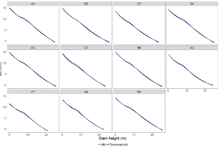
APPLIED TO EUCALYPTUS OF VARYING GENETICS IN BRAZIL ... 6 Figure 1. TECHS site distribution along different climatic zones in Brazil. ... 11 Figure 2. Comparison of the fitted equations for predicting stem taper for trees of different
eucalypt clones. ... 22 Figure 3. Performance of the fitted equation for predicting dib for trees of different eucalypt
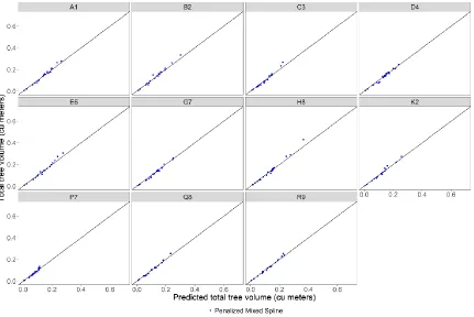
clones. ... 24 Figure 4. Comparison of the fitted equations for predicting total tree volume outside bark (m3)
with observed volume for trees of different eucalypt clones. ... 26 Figure 5. Performance of the fitted equation for predicting total tree volume inside bark (m3)
with observed volume for trees of different eucalypt clones. ... 27 Figure 6. Performance of the fitted equations for predicting total tree volume outside bark and
total tree volume inside bark (m3) with observed volume outside and inside bark for
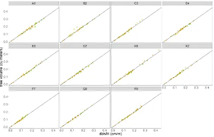
trees of different eucalypt clones. ... 29 Figure 7. Comparison of the fitted equations for predicting cumulative tree volume outside
bark (m3) for trees of different eucalypt clones. ... 32
Figure 8. Comparison of the fitted equations for predicting cumulative tree volume inside bark (m3) for trees of different eucalypt clones. ... 33 CHAPTER 3: YIELD PATTERN OF EUCALYPT CLONES ACROSS BRAZIL: AN
APPROACH TO CLONAL GROUPING ... 42 Figure 1. TECHS sites across tropical Brazil. ... 47 Figure 2. Three patterns of stand volume growth. ... 50 Figure 3 Agreement between the predicted volumes using all the fixed and random
coefficients of Eq. 2 and the observed stand volumes (m3.ha-1). ... 57 Figure 4. Volume yield of the clones along annual water deficit index (WDI) gradient. ... 58 Figure 5. Volume yield deviation of the clones across the TECHS sites (represented by WDI)
of the general group non-sensitive to climate variation a); and sensitive to climate variation b). ... 60 Figure 6. Volume yield pattern of the clones across the subgroups: high productivity a); and
xv Figure 7. Patterns of volume yields of the clonal groups across the annual water deficit index
(WDI) gradient a); linear trend of the clonal groups with decrease of WDI b). ... 64 CHAPTER 4: COMPATIBLE SET OF PREDICTION AND PROJECTION DOMINANT HEIGHT EQUATIONS FOR CLONAL EUCALYPT PLANTATIONS IN BRAZIL: A MODELING APPROACH EXPANDED AND REFINED BY ENVIRONMENTAL
VARIABLES ... 71 Figure 1. Distribution of TECHS sites along Brazil. ... 76 Figure 2. Dominant height growth of the clonal groups. ... 78 Figure 3. Prediction performance of the growth equations for different age classes (a) and (c);
projection performance of the growth equations along different projection lengths (b) and (d). ... 88 Figure 4. Prediction performance of the growth equations along different age classes (a)
and (c); projection performance of the growth equations along different projection lengths (b) and (d). ... 93 Figure 5. Agreement between the predicted and observed dominant heights at every clonal
group through the use of the: M2_2 model – 0th to 25th quantile age class a), 25th to 75th quantile age class c), and 75th to 100th quantile age class e); M2_2 model with the inclusion of SWD – 0th to 25th quantile age class b), 25th to 75th quantile age
class d), and 75th to 100th quantile age class f). ... 95 Figure 6. Agreement between the projected and observed dominant heights at every clonal
group through the use of the: M2_2 model – 0th to 25th quantile projection length a), 25th to 75th quantile projection length c), and 75th to 100th quantile projection length e); M2_2 model with the inclusion of SWD – 0th to 25th quantile projection length b), 25th to 75th quantile projection length d), and 75th to 100th quantile projection length f). ... 96 Figure 7. Prediction performance of the growth equations along different age classes (a) and
(c) using the rainfall exclusion plots; projection performance of the growth equations along different projection lengths (b) and (d) using the rainfall exclusion plots. ... 98 Figure 8. Agreement between the predicted and observed dominant heights at every clonal
group through the use of the: M2_2 model – 0th to 25th quantile age class a), 25th to 75th quantile age class c), and 75th to 100th quantile age class e); M2_2 model with the inclusion of SWD – 0th to 25th quantile age class b), 25th to 75th quantile age
class d), and 75th to 100th quantile age class f). ... 100 Figure 9. Agreement between the projected and observed dominant heights at every clonal
group through the use of the: M2_2 model – 0th to 25th quantile projection length a),
xvi 25th to 75th quantile projection length d), and 75th to 100th quantile projection length
f). ... 101 Figure 10. Site curves generated under three distinct average environmental scenarios
(SWD = -1209, -536 and -67 mm.year-1) along Brazil through the use of the prediction growth equation M2_2 with the inclusion of SWD (Eq. (14)), while the projection formulation is needed to make the family of polymorphic curves. ... 103 CHAPTER 5: MODELING WHOLE-STAND SURVIVAL IN CLONAL EUCALYPT
STANDS IN BRAZIL AS A FUNCTION OF WATER AVAILABILITY ... 112 Figure 1. Research sites installed along Brazil. ... 116 Figure 2. Stand survival (TPH) as a function of stand age (a); dominant height (b); and
cumulative soil water deficit (c) for every clonal group across the TECHS sites. ... 119 Figure 3. Projection performance of the difference equations N1 and N5 along different
projection lengths for the four clonal groups ... 128 Figure 4. Projection performance of the difference models N1 and N1 with cumulative SWD
(Eq. (10)) along different projection lengths applied to different SWD conditions (-184, -559, -1012 mm.year-1) for the clonal groups: A (a); B (b); C (c); and D (d). The high error for all clonal groups under the condition SWD = -1012 mm.year-1 is due to disease problems. ... 132 Figure 5. Whole-stand survival curves, by clonal groups, under three distinct SWD scenarios
(SWD = -1209, -536, and -67 mm.year-1) along the experimental research gradient of this study in Brazil using Eq. (16). To plug cumulative SWD in the fitted
difference equation: for the average SWD, SWD2 in year 6 = (6 x -536) =
-3216 mm. ... 134 CHAPTER 6: STAND-LEVEL GROWTH AND YIELD SYSTEM FOR CLONAL
EUCALYPT PLANTATIONS IN BRAZIL: A SYSTEM THAT ACCOUNTS FOR
WATER AVAILABILITY ... 142 Figure 1. TECHS sites along Brazil and northern Uruguay. ... 147 Figure 2. Basal area – m2.ha-1 (a) and stand volume – m3.ha-1 (b) productivity over time for
the four (A, B, C, D) clonal group across the TECHS sites. ... 149 Figure 3. Prediction performance of the growth equations across age classes (a); projection
performance of the growth equations along different projection lengths (b). ... 163 Figure 4. Agreement between the predicted and observed basal areas at every clonal group
xvii Figure 5. Agreement between the projected and observed basal areas at every clonal group
through the use of the: Eq. (5) – 0th to 25th quantile projection length a), 25th to 75th quantile projection length c), and 75th to 100th quantile projection length e); Eq. (7) – 0th to 25th quantile projection length b), 25th to 75th quantile projection length d), and 75th to 100th quantile projection length f). ... 166 Figure 6. Basal area curves generated under three distinct scenarios (SWD = -1209, -536 and
-67 mm.year-1) along Brazil through the use of the prediction Eqs. (5) and (7). This figure is based on the estimation of site index from Eq. (12) and stand survival from Eq. (14), recalling that stand survival for t=0 is 1111 trees per hectare. ... 168 Figure 7. Agreement between the predicted and observed stand volumes at every clonal group
through the use of the: Conventional G & Y system – 0th to 25th quantile age class a),
25th to 75th quantile age class c), and 75th to 100th quantile age class e); G & Y system with SWD – 0th to 25th quantile age class b), 25th to 75th quantile age class d), and 75th to 100th quantile age class f). The graphs were generated using exclusively the rainfall exclusion plots. ... 171 Figure 8. Agreement between the projected and observed stand volumes at every clonal group
through the use of the: Conventional G & Y system – 0th to 25th quantile projection length a), 25th to 75th quantile projection length c), and 75th to 100th quantile
projection length e); G & Y system with SWD – 0th to 25th quantile projection length b), 25th to 75th quantile projection length d), and 75th to 100th quantile projection length f). ... 172 Figure 9. Eucalyptus productivity in Brazil under different annual soil water deficit conditions:
-67 mm.year-1, -536 mm.year-1, and -1209 mm.year-1 for the four clonal groups (A, B, C, and D). This figure is based on the estimation of dominant height from Eq. (19), stand survival from Eq. (21), basal area from Eq. (22) and stand-level volume from Eq. (24), recalling that stand survival for t=0 is 1111 trees per
hectare. ... 175 CHAPTER 7: EUCALYPTUS GROWTH AND YIELD SYSTEM: LINKING
INDIVIDUAL-TREE AND STAND-LEVEL GROWTH MODELS IN CLONAL
EUCALYPT PLANTATIONS IN BRAZIL ... 182 Figure 1. Distribution of TECHS sites along Brazil. ... 187 Figure 2. Diagram of the compatible individual-tree and stand-level G & Y system. ... 196 Figure 3. Agreement between the predicted and observed diameter percentiles at every
clonal group through the use of the: Eq. (42) – 0th percentile - applied for prediction purposes a), Eq. (42) – 0th percentile - applied for projection purposes b), Eq. (36) –
10th percentile - applied for prediction purposes c), Eq. (37) – 10th percentile - applied for projection purposes d), Eq. (38) – 63rd percentile - applied for prediction purposes e), Eq. (39) – 63rd percentile - applied for projection purposes f),
xviii Figure 4. Agreement between the predicted and observed number of trees in the DBH
classes at every clonal group through the use of the Eq. (43)... 211 Figure 5. Agreement between the predicted and observed individual-tree heights at
every clonal group through the use of the Eq. (44)... 213 Figure 6. Average observed volumes at age 1.5 years a), average observed volumes at age 5
years b), projected volume estimates at age 5 years through the parameter recovery method c), projected volume estimates at age 5 years through the new stand table projection method d). Projection through the parameter recovery method (following the percentile methodology) was exemplified to demonstrate the superior and more realistic estimates provided by the new stand table projection method proposed in this study. ... 214 Figure 7. Comparison between the average observed volumes and the predicted volume
1 CHAPTER 1: INTRODUCTION
Eucalyptus cultivation is expanding in many regions of Brazil, however, much of the planted area demonstrates limitations to growth, notably when subject to different levels of water stress. Eucalyptus plantations are primarily clonal, and these clones are adapted to each of these regions, largely due to the genotype x environment (GxE) interaction. This results in complex decision making when selecting suitable genotypes for different environmental conditions (Stape et al., 2010).
The success of forest plantations, including the matching of genotypes to different climate and soil conditions, has a large impact on the economics of the enterprise and on the generation of social value to the local communities (Stape et al., 2010). In addition, in Brazil, the year-to-year variation in climate causes significant variability of the mean annual increment of clonal eucalypt plantations, which have an accelerated growth rate and high demand for water.
2 Montes (2012) tackled this task by developing a simultaneously fitted G & Y system driven by site resources, which was applied to estimate growth and yield for Pinus taeda plantations in SE USA. The G & Y system developed by Montes (2012) uses growth equations namely “statistical growth equations with physiologically derived covariates” (Weiskittel et al., 2011), where the age term of the growth equations is replaced by growth modifiers derived from 3-PG (Landsberg and Warring, 1997). Casnati (2016) developed a similar system for Pinus taeda and Eucalyptus grandis in Uruguay, although the author used radiation sums instead of having a modeling compartment for leaf area index. The major drawback displayed by the hybrid approach is associated with compounding error through the use of site resource variables, instead of stand age, to describe forest growth.
This approach, however, appears to be very attractive for fitting stand survival equations to clonal eucalypt stands in Brazil, since the eucalyptus survival rate is not well correlated to site index, as observed by Casnati (2016). It is typically hypothesized that a certain level of water stress induces higher tree mortality in clonal eucalypt stands. Thus, the replacement of the age term in the survival model by a variable that represents the dynamics of water availability over time, might potentially result in more biologically sound survival estimation. It is also hypothesized that a single variable to representing stand mortality might mitigate the compounding error problem.
3 water availability in the site index model, substantially increased the explanatory ability of the fitted model.
A simplified hybrid approach for stand survival estimation combined to dominant height and basal area equations expanded and refined by environmental variables that reflects how water availability impacts forest productivity, appears to be an attractive form to build a G & Y system for clonal eucalypt plantations in Brazil. This type of G & Y system, governed by water availability, predicts forest yield for afforestation and updates forest inventory spanning Brazil as well as displays consistency between individual-tree and stand-level estimates. The growth equations may employ mixed effect modeling to also account for clonal variation.
Thus, the goal of this dissertation is to provide a framework for addressing the genotype x environment interaction in a G & Y system for clonal eucalypt plantations in Brazil. This results in a system that is sensitive to clonal and climate variation, and capable of providing either stand level or stand structure estimates for the entire geographic extent of Brazil. It is worth mentioning that the goal is to produce a simple, yet complete G & Y system. The specific goals of the dissertation are:
1) To develop generalized total tree and merchantable volume equations and generalized taper equations for eleven eucalypt clones spanning tropical Brazil (Chapter 2).
2) To evaluate if it is feasible to group the 11 clones into 2 or more groups that share similar yield patterns (Chapter 3).
3) To develop a compatible set of prediction and projection equations capable of accounting for how water availability changes the dominant height tree growth trajectory (Chapter 4). 4) To develop a whole-stand survival equation that is a function of water availability
4 5) To develop a stand-level G & Y system, governed by water availability, that is capable of predicting forest yield for afforestation and updating forest inventory for all of Brazil (Chapter 6).
5 REFERENCES
Casnati, A.C.R., 2016. Hybrid mensurational-physiological models for Pinus taeda and
Eucalyptus grandis in Uruguay. PhD Dissertation. University of Canterbury, Canterbury, New Zealand, 208 p.
Landsberg, J.J., Waring, R.H., 1997. A generalised model of forest productivity using simplified concepts of radiation-use efficiency, carbon balance and partitioning. For. Ecol. Manage. 95, 209–228.
Montes, C.R., 2012. A Resource Driven Growth and Yield Model for Loblolly Pine Plantations. PhD Dissertation. North Carolina State University, Raleigh, USA, 87 p.
Scolforo, H.F., Castro Neto, F., Scolforo, J.R.S., Burkhart, H., McTague, J.P., Raimundo, M.R., Loos, R.A., Fonseca, S., Sartorio, R.C. 2016. Modeling dominant height growth of eucalyptus plantations with parameters conditioned to climatic variations. For. Ecol. Manage. 380, 182–195
Scolforo, H.F., Scolforo, J.R.S., Stape, J.L., McTague, J.P., Burkhart, H., McCarter, J., Neto, Fd.C., Loos, R.A., Sartorio, R.C., 2017. Incorporating rainfall data to better plan Eucalyptus clones deployment in eastern Brazil. For. Ecol. Manage. 391, 145–153. Snowdon, P., Woollons, R.C., Benson, M.L., 1998. Incorporation of climatic indices into models
of growth of Pinus radiata in a spacing experiment. New For. 16, 101-123.
Stape JL et al. 2010. The Brazil Eucalyptus Potential Productivity Project: Influence of water, nutrients and stand uniformity on wood production. For. Ecol. Manage. 259, 1684-1694. Weiskittel, A.R., Hann, D.W., Kershaw Jr, J.A., Vanclay, J.K., 2011. Forest growth and yield
6 CHAPTER 2: GENERALIZED STEM TAPER AND TREE VOLUME EQUATIONS
APPLIED TO EUCALYPTUS OF VARYING GENETICS IN BRAZIL
Abstract: Volume and taper equations have been widely applied with a variety of model forms. Lack of generalized equations has prevailed in Brazil, since it is assumed that localized or climate-specific equations are needed. The lack of generalized equations, however, limit the prediction of stem taper, merchantable and total tree volume of the most widely planted eucalypt clones along Brazil. Thus, this study aimed to develop generalized stem taper and volume equations applicable to eleven eucalyptus clones and evaluate if climate variation impacts the accuracy of the estimates. A total of 693 trees evenly distributed across eleven clones at 21 sites were used, where 462 and 231 trees were used for model fittings and predictive validation, respectively. The penalized mixed spline (PMS) approach was developed for predicting stem taper, and volume along the stem profile. The Schumacher and Hall (1933) equation was used to predict total tree volume, while volume ratio equations were applied to predict merchantable volume up to any top diameter or stem height. For every fitted equation, a climatic variable on an annual basis, was included to assess the improvement in model performance. The overall results highlighted that climatic variation does not need to be accounted for in stem taper and volume modeling. The climatic impact is already fully captured by the fitted coefficients of the equations. All the equations displayed desirable accuracy, whereas the generalized PMS equation may be preferred when the forestry enterprise looks to furnish a range of multiple forest products. The generalized total tree volume equation, combined with the ratio equations, is highly recommended when the forestry enterprise produces a single product.
7 1. Introduction
Stem taper and tree volume equations are valuable tools that enhance the efficiency of forest management decision making and maximizing profit of a forestry enterprise (Burkhart and Tomé, 2012). Depending upon the forestry enterprise goals the equations are: 1) customarily used to complement and increase the level of information provided by forest inventory; 2) linked to sequential inventory information to allow the development of growth and yield models with different merchantability standards (Casnati, 2016).
For commercial plantations focused on the production of a single product, there is no need for having highly detailed information. A set of readily available total and merchantable volume tree equations is preferable for parsimony, simplicity and accurate estimation (Bullock and Burkhart, 2003). According to Azevedo et al. (2011), merchantable and total tree volume equations in Brazil are customarily fitted independently, which increases the possibility of illogical crossing of the estimated values. The use of dummy variables that allow estimation of total and merchantable tree volume in a single equation has been proposed to fix this possible shortcoming and the observed results are satisfactory (Figueiredo, 2005). The problem associated with the use of such tree volume equations is that they are only able to estimate merchantable tree volume up to a fixed top diameter or upper-stem height (Burkhart and Tomé, 2012), in which the Schumacher and Hall (1933) tree volume equation is customarily used (Lee et al., 2017).
8 diameter. Cao and Burkhart (1980) noticed that product classes may be defined according to the log length instead of top diameter. Thus, the authors formulated a volume ratio model that is able to estimate merchantable volume at any given stem height. Zhao and Kane (2017) proposed a similar formulation for Pinus taeda in the southern USA, while including a constraint that volume should be zero when top diameter is specified at ground height.
Bullock and Burkhart (2003) demonstrated that combining the set of equations: 1) exponential ratio model of Van Deusen et al. (1981), 2) volume ratio based on upper-stem height proposed by Cao and Burkhart (1980), and 3) total tree volume equation, enables accurate volume estimates, while avoiding the illogical crossing of merchantable and total tree volume estimates. The authors indeed provided a set of equations that can accurately estimate green weight at any stem height and top diameter. They also implicitly derived a taper function, which performs well over much of the stem for diameter estimation, with some sacrifice of weight estimation for the first logs.
9 Despite the great variety of stem taper equations, Scolforo et al. (2018) suggested the use of the penalized mixed spline approach. The authors highlighted the great flexibility and stability of such approach to predict eucalyptus stem taper of varying genetics in southern Brazil. Since eucalyptus trees display a tremendous yearly growth rate, a dramatic annual change in tree size is also observed, which implies a further indication of the flexibility of the PMS approach.
A casual observation reveals the existence of two different foci regarding forest production in Brazil (Carvalho et al., 2005). One is directly influenced by the Asian market demand, while the second one is related to the idea of diversifying the range of products generated by the forest. Several tree volume and stem taper equations have been developed under specific genetics and geographical areas (Assis et al., 2001). The authors noted however, a lack of studies focused on the development of generalized stem taper and tree volume equations, especially for varying genetics and expansive areas with great climate variation. The authors, on contrary of Bullock and Burkhart (2003), assumed that equations specific to each genetic material and for every specific geographic regions should be fitted. Scolforo et al. (2018) pointed out, however, that there is no decrease in accuracy by using a single, generalized equation applied to eucalyptus of varying genetics for the southernmost part of Brazil. Thus, the remaining question consists in understanding if climate variables indeed display significant improvement in the accuracy of the estimates and if such variables should be included or not to reduce bias when proposing generalized equations in Brazil.
10 by Cao and Burkhart (1980) and Van Deusen et al. (1981) were used to directly estimate total tree and merchantable volume.
2. Material and methods 2.1. Database
This data comes from 21 (1, 2, 3, 4, 5, 7, 8, 9, 11, 13, 14, 15, 17, 19, 22, 24, 26, 29, 30, 31 and 33) experimental sites of the TECHS Project (Tolerance of Eucalyptus Clones to Hydric, Thermal and Biotic Stresses, www.ipef.br/techs/en), which was launched in 2011 in Brazil (Binkley et al., 2017). TECHS basically divided Brazil in two strata: tropical and subtropical. For tropical Brazil, sites ranged from Paraná to Pará State (Figure 1). This range encompasses all Brazilian climate zones where eucalyptus can grow. There are sites in Köppen climate regions such as Am (tropical zone – monsoon), As (tropical zone – with dry summer), Aw (tropical zone – with dry winter), Cfa (humid subtropical zone with hot summer and without dry season), Cfb (humid subtropical zone with temperate summer and without dry season), Cwa (humid subtropical zone with hot summer and dry winter), and Cwb (humid subtropical zone with temperate summer and dry winter) (Alvares et al., 2013).
11 Figure 1. TECHS site distribution along different climatic zones in Brazil.
The experimental sites were installed between January and May of 2012. At each site, eleven different clones (A1, B2, C3, D4, E5, G7, H8, K2, P7, Q8 and R9) were planted in clone specific block plots. A single plot consists of 80 trees spaced at 3 x 3 meters. Additionally, one plot edge with 8 trees was installed for destructive sampling, where the eucalyptus trees at approximately age 3 years were bucked and scaled.
A total of 693 trees, evenly distributed across every TECHS site and clones, were bucked and scaled during 2015. For each TECHS site and for every clone, trees were selected across a range of tree size classes, with equal representation for the 25th dbh percentile, 50th dbh percentile
12 outside bark (dob) and bark thickness were measured at stump height, at 1.3m, and at the middle height of the tree. The geometric method proposed by Andrade et al. (2006) allowed recovering dob and dib after 1.3m at every 2m until the tree top.
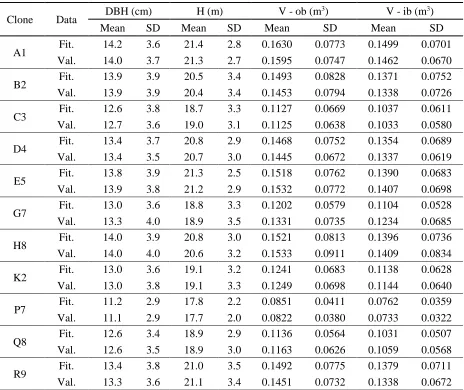
Table 1. Descriptive statistics for each clone of the eucalyptus plantations.
Clone Data DBH (cm) H (m) V - ob (m
3) V - ib (m3)
Mean SD Mean SD Mean SD Mean SD
A1 Fit. 14.2 3.6 21.4 2.8 0.1630 0.0773 0.1499 0.0701 Val. 14.0 3.7 21.3 2.7 0.1595 0.0747 0.1462 0.0670
B2 Fit. 13.9 3.9 20.5 3.4 0.1493 0.0828 0.1371 0.0752 Val. 13.9 3.9 20.4 3.4 0.1453 0.0794 0.1338 0.0726
C3 Fit. 12.6 3.8 18.7 3.3 0.1127 0.0669 0.1037 0.0611 Val. 12.7 3.6 19.0 3.1 0.1125 0.0638 0.1033 0.0580
D4 Fit. 13.4 3.7 20.8 2.9 0.1468 0.0752 0.1354 0.0689 Val. 13.4 3.5 20.7 3.0 0.1445 0.0672 0.1337 0.0619
E5 Fit. 13.8 3.9 21.3 2.5 0.1518 0.0762 0.1390 0.0683 Val. 13.9 3.8 21.2 2.9 0.1532 0.0772 0.1407 0.0698
G7 Fit. 13.0 3.6 18.8 3.3 0.1202 0.0579 0.1104 0.0528 Val. 13.3 4.0 18.9 3.5 0.1331 0.0735 0.1234 0.0685
H8 Fit. 14.0 3.9 20.8 3.0 0.1521 0.0813 0.1396 0.0736 Val. 14.0 4.0 20.6 3.2 0.1533 0.0911 0.1409 0.0834
K2 Fit. 13.0 3.6 19.1 3.2 0.1241 0.0683 0.1138 0.0628 Val. 13.0 3.8 19.1 3.3 0.1249 0.0698 0.1144 0.0640
P7 Fit. 11.2 2.9 17.8 2.2 0.0851 0.0411 0.0762 0.0359 Val. 11.1 2.9 17.7 2.0 0.0822 0.0380 0.0733 0.0322
Q8 Fit. 12.6 3.4 18.9 2.9 0.1136 0.0564 0.1031 0.0507 Val. 12.6 3.5 18.9 3.0 0.1163 0.0626 0.1059 0.0568
R9 Fit. 13.4 3.8 21.0 3.5 0.1492 0.0775 0.1379 0.0711 Val. 13.3 3.6 21.1 3.4 0.1451 0.0732 0.1338 0.0672
SD: standard deviation; V - ob: total volume outside bark; V - ib: total volume inside bark; Fit.: fitting dataset; and
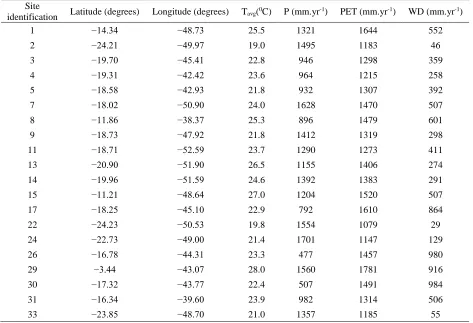
13 Weather stations were installed at every TECHS site during the experiment installation. Weather information recorded on a daily basis has provided information such as: precipitation (P in mm), average temperature (Tavg, 0C), potential evapotranspiration (PET, mm) and water deficit
(WD, mm) (Table 2).
Table 2. Climate description of the TECHS sites.
Site
identification Latitude (degrees) Longitude (degrees) Tavg(
0C) P (mm.yr-1) PET (mm.yr-1) WD (mm.yr-1)
1 −14.34 −48.73 25.5 1321 1644 552
2 −24.21 −49.97 19.0 1495 1183 46
3 −19.70 −45.41 22.8 946 1298 359
4 −19.31 −42.42 23.6 964 1215 258
5 −18.58 −42.93 21.8 932 1307 392
7 −18.02 −50.90 24.0 1628 1470 507
8 −11.86 −38.37 25.3 896 1479 601
9 −18.73 −47.92 21.8 1412 1319 298
11 −18.71 −52.59 23.7 1290 1273 411
13 −20.90 −51.90 26.5 1155 1406 274
14 −19.96 −51.59 24.6 1392 1383 291
15 −11.21 −48.64 27.0 1204 1520 507
17 −18.25 −45.10 22.9 792 1610 864
22 −24.23 −50.53 19.8 1554 1079 29
24 −22.73 −49.00 21.4 1701 1147 129
26 −16.78 −44.31 23.3 477 1457 980
29 −3.44 −43.07 28.0 1560 1781 916
30 −17.32 −43.77 22.4 507 1491 984
31 −16.34 −39.60 23.9 982 1314 506
33 −23.85 −48.70 21.0 1357 1185 55
2.2. Tree volume and stem taper equations
14 In particular, Chi and Reinsel (1989) suggested the additional use of the first-order continuous autocorrelation function (CAR1) and power variance function in cases where mixed effect modeling technique does not eliminate the total within-stem correlation and variance heteroskesdaticity effects. Their suggestions were employed in the fitting of PMS, dib and volume ratio equations.
2.2.1. Tested climatic variables
The variables Tavg, PET, P and WD were the variables used to test the environmental impact
on the accuracy of the estimates. The presumed null hypothesis is that none of these variables impact stem taper and volume predictions for any clone across Brazil.
The variables P and PET were combined in a single variable as (P - PET), which provides a measure of the vertical atmospheric pressure. The variable WD integrates physiographic and climatic variables, which makes this variable an extremely powerful co-variate. Tavg can be used
as a good predictor, since this variable is indicative of climatic difference and seasonality in Brazil. For simplicity, the tested climatic variables were generally labeled as CV through the following methods sections.
2.2.2. Penalized Mixed Spline (PMS)
15 is obtained through the estimated best linear unbiased predictor (EBLUP), since
p uk
= , which
consists in the maximizing likelihood of the PMS.
Scolforo et al. (2018) applied such an approach to model stem taper of a variety of eucalypt clones in the southernmost part of Brazil; the authors reported on the flexible nature of the approach. The development of the PMS approach is related to the Max and Burkhart (1976) splined taper concept; however, this approach easily allowed additional knots to account for flare in the bottom portion of the stem.
Differing from the original formulation presented by Scolforo et al. (2018), previous tests of this research indicated that using 3 empirical knots are sufficient (l1 = 0.10, l2 = 0. 75, l3 = 0.97), which ensures a parsimonious equation. Equation (1) is a linear mixed model, where the variable
2
ln 2 10000
ijk ijk hijk
ijk
DBH H h H −
is fixed, the quadratic expression is declared random based on clones, and the
knots are declared random based on tree (TECHS site) 1 and TECHS site.
2 2 2
1 1 2 2 3 l_
1
( ) 1 ( ) 1 ln 2 1
L
hijk hijk hijk hijk hijk
j j ijk ijk ik l hijk
l
ijk ijk ijk ijk ijk
d h h h h
b b DBH H u l
DBH H H H = H
+ = + − + + − + − + − − + (1)
where, subscripts h, i, j and k refer to stem height h of tree i of clone j of TECHS site k;
𝛽1, 𝛽2 𝑎𝑛𝑑 𝛽3 = fixed coefficients to be estimated; 𝑏1𝑗 𝑎𝑛𝑑𝑏2𝑗 = random coefficients based on clone; L = 3 knots; dhijk = upper-stem diameter outside bark; ul_ik are the random coefficients
associated with knots based on tree (TECHS site) and TECHS site; the + subscript operator implies that the function is computed if 1 - (hhijk/Hijk) is larger than the knot value inside the parenthesis,
16 otherwise the value is zero; other variables were previously defined; 𝜀ℎ𝑖𝑗𝑘~𝑁(0, 𝜎2𝐼), 𝑏𝑖𝑗~𝑁(0, 𝜎2𝐷) and 𝑢
𝑙_𝑖𝑘~𝑁(0, 𝜎2𝐷).
To include the impact of climatic variables in the stem taper equation, the coefficient associated with tree size was decomposed to include the CV. CV was included this way, to ensure that at the tree tip the stem diameter is zero.
2 2
2
1 1 2 2 3 4 l_
1
( ) 1 ( ) 1 ( ) ln 2 1
L
hijk hijk hijk hijk hijk
j j k ijk ijk ik l hijk
l
ijk ijk ijk ijk ijk
d h h h h
b b CV DBH H u l
DBH H H H = H
+ = + − + + − + + − + − − + (2)
where, 𝐶𝑉 stands for every tested climate variable associated with every k TECHS site; other variables were previously defined.
The formulation above permits the estimation of diameter outside bark (dob) at any stem height. The formulation below is proposed to estimate diameter inside bark (dib) at any stem height, where tree size was included to increase the equation flexibility regarding dib/dob ratio. Equation (3) is a linear mixed model, where dob is declared random based on tree (clones) 2 and clones.
2
1 1 3
( ) ln 2
10000
ijk ijk hijk
hijk ij hijk hijk
ijk
DBH H h
dib b d
H
= + + − +
(3)
where, all the variables were previously defined. Eq (3) logically predicts that dib = 0 at the tip of tree.
17 The PMS approach possesses a tedious lengthy closed-form integral, hence volume, outside and inside bark in m3, was calculated through Smalian´s formula, where numerical integration followed the same intervals applied in the destructive samples.
2.2.3. Total and merchantable volume models
The allometric equation proposed by Schumacher and Hall (1933) was used for total tree volume estimation. The non-linear equation, however, was linearized by log transformation. The linearized form of the equation is usually applied for eucalyptus in Brazil for reasons of simplicity (Vismara et al., 2015).
The linear version of the individual tree volume equation [Equation (4)] was fitted as a normal linear mixed model, where the expression for the intercept is declared random based on tree (clones) 3, clones.
𝑙𝑛(𝑣𝑖𝑗𝑘) = (𝛽0+ 𝑏0𝑖𝑗) + (𝛽01+ 𝑏01𝑖𝑗)𝐼1+ 𝛽1𝑙𝑛(𝐷𝐵𝐻𝑖𝑗𝑘) + 𝛽2𝑙𝑛(𝐻𝑖𝑗𝑘) + 𝜀𝑖𝑗𝑘 (4) where, 𝑣 is total individual tree volume outside and inside bark in m3; DBH = diameter at 1.30 m
aboveground in cm; H = total height in m; subscripts i, j and k refer to tree i of clone j of TECHS site k; 𝛽0, 𝛽01, 𝛽1 𝑎𝑛𝑑𝛽2= fixed coefficients to be estimated; 𝑏0𝑖𝑗 𝑎𝑛𝑑𝑏01𝑖𝑗 = random coefficients based on tree (clone) and clone; 𝐼1 is a dummy variable associated with the intercept for the
estimation of volume inside bark; 𝜀𝑖𝑗𝑘~𝑁(0, 𝜎2𝐼) and 𝑏
𝑖𝑗~𝑁(0, 𝜎2𝐷).
18 This results in a general total tree volume equation, which is a new approach in Brazil, since volume equations are traditionally fit and localized for each forest compartment (Kohler et al., 2016).
To account for the impact of the climatic variables in the volume estimation, the linearized form of the Schumacher and Hall (1933) equation included an extra term regarding these variables. This resulted in one fitted equation per CV, which means that three equations were fit with the purposes to include a climatic covariate.
𝑙𝑛(𝑣𝑖𝑗𝑘) = (𝛽0+ 𝑏0𝑖𝑗) + (𝛽01+ 𝑏01𝑖𝑗)𝐼1+ 𝛽1𝑙𝑛(𝐷𝐵𝐻𝑖𝑗𝑘) + 𝛽2𝑙𝑛(𝐻𝑖𝑗𝑘) + 𝛽3𝐶𝑉𝑘+ 𝜀𝑖𝑗𝑘 (5)
where, 𝐶𝑉 stands for every tested climatic variable associated with every k TECHS site; other variables were previously defined.
There is a lack of reliable volume equations for predicting merchantable volume up to any top diameter or upper-stem height for eucalyptus in Brazil. Thus, the suggested use of ratio equations for tree species in Brazil represents another feature of this study. The non-linear version of the ratio volume equations [Equations (6) and (7)] were fitted as non-linear mixed models, where the expressions for the intercepts were declared random based on tree (clones) 4 and clones.
19 𝑚𝑣ℎ𝑒𝑖𝑔ℎ𝑡_ℎ𝑖𝑗𝑘 = 𝑣𝑖𝑗𝑘𝑒𝑥𝑝 (1−(𝛼1+𝑎1𝑖𝑗)(𝐻𝑖𝑗𝑘−ℎℎ𝑖𝑗𝑘)
𝛼2
𝐻𝑖𝑗𝑘𝛼3 ) +𝜀ℎ𝑖𝑗𝑘 (6) 𝑚𝑣𝑑𝑖𝑎𝑚𝑒𝑡𝑒𝑟_ℎ𝑖𝑗𝑘 = 𝑣𝑖𝑗𝑘𝑒𝑥𝑝 ((𝛽4+𝑏4𝑖𝑗) 𝑑ℎ𝑖𝑗𝑘
𝛽5
𝐷𝐵𝐻𝑖𝑗𝑘𝛽6) + 𝜀ℎ𝑖𝑗𝑘 (7) where, 𝑚𝑣ℎ𝑒𝑖𝑔ℎ𝑡 merchantable volume, outside and inside bark in m3, to any upper height; 𝑚𝑣𝑑𝑖𝑎𝑚𝑒𝑡𝑒𝑟 merchantable volume, outside and inside bark in m3, to any top diameter; dhijk upper-stem diameter outside and inside bark in cm; hhijk is the upper-stem height in m;
𝛼1, 𝛼2, 𝛼3, 𝛽4, 𝛽5 𝑎𝑛𝑑𝛽6 = fixed coefficients to be estimated; 𝑎1𝑖𝑗 𝑎𝑛𝑑𝑏4𝑖𝑗 = random coefficients based on tree (clone), and clone; subscripts h refers to stem height and diameter, respectively, of tree i of clone j of TECHS site k; 𝜀ℎ𝑖𝑗𝑘~𝑁(0, 𝜎2), 𝑎
𝑖𝑗~𝑁(0, 𝜎2𝐷) and 𝑏𝑖𝑗~𝑁(0, 𝜎2𝐷).
2.3. Goodness of fit
20 𝑇 = 1
𝑛∑ (𝑂 − 𝑃𝑟)
𝑛
𝑖=1 (8)
𝑀𝐴𝐸 = 1
𝑛∑ |𝑂 − 𝑃𝑟|
𝑛
𝑖=1 (9)
𝑅𝑀𝑆𝐸 = √∑𝑛𝑖=1(𝑃𝑟−𝑂)2
𝑛 (10)
𝐸𝐹 = 1 −∑𝑛𝑖=1(𝑂−𝑃𝑟)2
∑𝑛 (𝑂−𝑂̅)2 𝑖=1
(11) where, 𝑃𝑟 is the predicted values; 𝑂 is the observed values; 𝑂̅is the average of observed values; 𝑛
is the number of observations.
T, MAE and RMSE closer to zero and EF closer to 1 indicate a better fit. Graphical analysis, through the use of the R package ggplot2 (Wickham, 2009), were also conducted to evaluate the overall predictions.
3. Results
3.1. Stem taper predictions over different clones
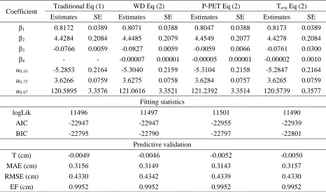
Table 3 displays the overall results for all fitted equations. Except for β4 of the stem taper
equation that included Tavg, all the other coefficients for all stem taper equations are significant
21 Table 3. Fitted coefficients with their standard errors (SE) of Equations 1-2, and goodness of fit indicators (logLik, AIC, BIC, T, MAE, RMSE and EF).
Coefficient Traditional Eq (1) WD Eq (2) P-PET Eq (2) Tavg Eq (2)
Estimates SE Estimates SE Estimates SE Estimates SE
β1 0.8172 0.0389 0.8071 0.0388 0.8047 0.0388 0.8173 0.0389
β2 4.4284 0.2084 4.4485 0.2079 4.4549 0.2077 4.4278 0.2084
β3 -0.0766 0.0059 -0.0827 0.0059 -0.0059 0.0066 -0.0761 0.0300
β4 - - -0.00007 0.00001 -0.00005 0.00001 -0.00002 0.0010
u0.10 -5.2853 0.2164 -5.3040 0.2159 -5.3104 0.2158 -5.2847 0.2164
u0.75 3.6266 0.0759 3.6275 0.0758 3.6284 0.0757 3.6265 0.0759
u0.97 120.5895 3.3576 121.0616 3.3521 121.2392 3.3514 120.5739 0.3577
Fitting statistics
logLik 11496 11497 11501 11490
AIC -22947 -22947 -22955 -22939
BIC -22795 -22790 -22797 -22801
Predictive validation
T (cm) -0.0049 -0.0046 -0.0052 -0.0050
MAE (cm) 0.3156 0.3149 0.3143 0.3157
RMSE (cm) 0.4330 0.4342 0.4339 0.4330
EF (cm) 0.9952 0.9952 0.9952 0.9952
The stem taper equation with the (P-PET) climatic variable displayed the overall best results in the fitting process, although the gain in precision over the Eq. (1) was minor. Meanwhile, in the predictive validation, high accuracy was still obtained when modeling stem taper without the inclusion of the climatic variable. The overall estimates of every stem taper equation across all the TECHS sites and clones showed minimum bias, high model efficiency, and lower MAE and RMSE. Irrespective of the approach used to describe the shape of the tree bole; T was never greater than -0.0052cm, EF was never lower than 0.9952, while RMSE and MAE were always lower than 0.43 cm.
22 clones. The average estimates generated by every stem taper equation basically overlapped, which is in agreement with the findings observed in Table 3. It might be preferred to keep using the generalized stem taper equation without any climatic variable included. Including climatic variables resulted in a minimal gain in accuracy, and by eliminating such variables it is possible to have a parsimonious fitted equation with the same predictive ability.
Differences in tree shape, height and diameter for the TECHS sites are accounted for in the coefficients of the fitted PMS model without any climatic variable. The PMS approach provides great flexibility by including knots that describe the profile change of the tree bole and by including a tree size variable ( 2
ln 2 10000
DBH H h
H
−
).
23 In order to estimate dib at any stem height, a specific equation relating this variable to dob and 2
ln 2 10000
DBH H h
H
−
was fitted. The coefficients of the fitted equation were significant and showed
low standard errors (Table 4). To the predictive validation, however, we decided to use the estimated dob values generated by the generalized PMS equation (Eq. (1)), instead of the observed dob values, as the inputs for the dib equation. Using such criteria allowed inspection of the impact of the compounding error from the generalized PMS estimates into the dib estimation.
Table 4. Fitted coefficients with their standard errors (SE) of Eq. (3), and goodness of fit indicators (logLik, AIC, BIC, T, MAE, RMSE and EF) to predict dib at any stem height.
Coefficient Estimates SE
β1 0.8386 0.0019
β2 4.1429 0.0781
Fittings statistics
logLik 6369
AIC -12727
BIC -12687
Predictive validation
T (cm) -0.0207
MAE (cm) 0.3394
RMSE (cm) 0.4871
EF 0.9928
24 Figure 3. Performance of the fitted equation for predicting dib for trees of different eucalypt clones.
3.2. Total tree volume prediction based on the generalized PMS taper functions and diameter inside bark equations
The generalized PMS equation without a climatic variable allowed accurate stem taper estimation (dob) overall for the different clones and TECHS sites. However, it is critical to check if the desired accuracy is maintained in the total tree volume prediction. As previously mentioned, the inclusion of climatic variables did not increase the accuracy of the estimates.
25 Table 5. Goodness of fit indicators (T, MAE, RMSE and EF) to predict total tree volume outside bark (Traditional, WD, P-PET, Tavg) and inside bark volume (vib), in m3.
Statistics Traditional WD P-PET Tavg vib*
T (m3) 0.0002 0.0003 0.0003 0.0002 0.0208
MAE (m3) 0.0056 0.0056 0.0056 0.0056 0.0209
RMSE (m3) 0.0081 0.0081 0.0081 0.0081 0.0229
EF 0.9889 0.9889 0.9887 0.9989 0.9099
*the input variable dob was computed using the traditional generalized PMS equation (Eq. 1)
26 Figure 4.Comparison of the fitted equations for predicting total tree volume outside bark (m3) with
27 Figure 5. Performance of the fitted equation for predicting total tree volume inside bark (m3) with
observed volume for trees of different eucalypt clones.
3.3. Total tree volume prediction over different clones by the Schumacher and Hall (1933) equation
Table 6 displays the overall fit results of fitted Equations 4-5. Again, the coefficient β3 for
the climatic variable (Tavg) is the only one not significant. All the other coefficients for every total
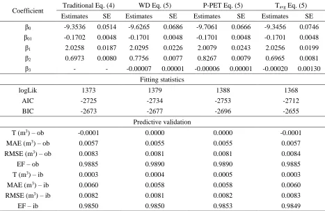
28 Table 6. Fitted coefficients with their standard errors (SE), and goodness of fit indicators for Equations 4-5 (logLik, AIC, BIC, T, MAE, RMSE and EF).
Coefficient Traditional Eq. (4) WD Eq. (5) P-PET Eq. (5) Tavg Eq. (5) Estimates SE Estimates SE Estimates SE Estimates SE β0 -9.3536 0.0514 -9.6265 0.0686 -9.7061 0.0666 -9.3456 0.0746
β01 -0.1702 0.0048 -0.1701 0.0048 -0.1701 0.0048 -0.1701 0.0048
β1 2.0258 0.0187 2.0295 0.0226 2.0079 0.0243 2.0256 0.0199
β2 0.6973 0.0080 0.7756 0.0077 0.8267 0.0079 0.6965 0.0081
β3 - - -0.00007 0.00001 -0.00006 0.00001 -0.00020 0.00130
Fitting statistics
logLik 1373 1379 1388 1368
AIC -2725 -2734 -2753 -2712
BIC -2673 -2677 -2696 -2655
Predictive validation
T (m3) – ob -0.0001 0.0000 0.0000 -0.0001
MAE (m3) – ob 0.0057 0.0055 0.0055 0.0057
RMSE (m3) – ob 0.0083 0.0081 0.0081 0.0084
EF – ob 0.9885 0.9890 0.9890 0.9885
T (m3) – ib 0.0003 0.0004 0.0005 0.0003
MAE (m3) – ib 0.0060 0.0058 0.0058 0.0060
RMSE (m3) – ib 0.0082 0.0081 0.0082 0.0083
EF – ib 0.9850 0.9850 0.9853 0.9849
29 Figure 6 reflects the performance behavior and virtually ensures the same prediction performance of all tested equations. There is no need to add an extra variable for climatic variation for total tree volume estimation, since the predictions from the different tested equations overlapped and performed well for every clone. As a result, the generalized total tree volume equation without any climatic variable is proposed for the estimation of total volume inside and outside bark.
Figure 6.Performance of the fitted equations for predicting total tree volume outside bark and total tree volume inside bark (m3) with observed volume outside and inside bark for trees of different eucalypt clones.
30 noticed. It is worth noting, however, the vib estimation, where the generalized Schumacher and Hall (1933) equation displayed higher accuracy. This suggests the use of the Schumacher and Hall (1933) equation if it is aimed solely to predict total tree volume. Additionally, this single equation is simpler to use, which makes possible error propagation less frequent.
3.4. Volume ratio predictions and comparison of these equations with the generalized PMS taper model and diameter inside bark equations
31 Table 7. Fitted coefficients with their standard errors (SE), and goodness of fit indicators for Equations 6-7 (logLik, AIC, BIC, T, MAE, RMSE and EF).
Upper stem height Top diameter
Coefficient Estimates SE Coefficient Estimates SE
α1 1.0915 0.0064 β4 -0.6349 0.0288
α2 2.5947 0.0018 β5 5.2876 0.0242
α3 2.6265 0.0025 β6 4.8945 0.0301
Fitting statistics
logLik 52451 35337
AIC -104892 -70664
BIC -104856 -70628
Predictive validation
T (m3) – ob 0.0001 0.0037
MAE (m3) – ob 0.0031 0.0074
RMSE (m3) – ob 0.0053 0.0108
EF – ob 0.9959 0.9832
T (m3) – ib 0.0003 -0.0047
MAE (m3) – ib 0.0034 0.0076
RMSE (m3) – ib 0.0056 0.0109
EF - ib 0.9939 0.9767