Determination of fracture toughness curve using R-6 method

(1)

DETERMINATION OF FRACTURE TOUGHNESS CURVE USING R-6

FAILURE ASSESSMENT METHOD

M. K. Sahu, J. Chattopadhyay and B. K. Dutta

Reactor Safety Division, Bhabha Atomic Research Centre, Mumbai, India

ABSTRACT

Determination of fracture property, J-R curve from experimental test results requires certain geometry factors. These expressions of geometry factors are available for standard geometries and loading configurations. However, for complex geometries and loading configurations these expressions are not available in open literature. R-6 Failure Assessment Diagram (FAD) methodology is used for assessment of failure in terms of mainly ductile crack initiation point. The use of this method is extended to estimate the entire J-R curve from the fracture test results. Under comprehensive test program initiated at RSD (Reactor Safety Division), BARC (Bhabha Atomic Research Centre), large numbers of straight pipes with circumferential cracks have been tested. These experimental results have been used to calculate material J-R curves using J-R-6 FAD, which are subsequently compared with conventional J-J-R curves calculated by !

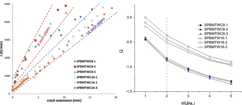
factor approach. It can be observed that the J-R curves calculated using both approaches are mostly in good agreements. Further, the segregation of J-R curves based on the size of pipes has been studied in the light of prevalent crack tip constraints. Here, crack tip constraints are calculated in terms of stress triaxiality parameters, Q for all pipes. It can be noted that the J-R curves for 8 inch pipes are higher because they have lower constraints than 16 inch pipes, which establishes the theory that high/low crack tip constraint causes low/high material fracture toughness.

INTRODUCTION

(2)

approach requires experimental load vs. crack extension data and, stress intensity factor, !, fracture toughness, Kmat, and limit load, "_#. The closed form expressions of stress intensity factor, !, and limit load,

"# are available for wide range of geometries in the literature. Thus, proposed methodology can be used easily for determination of fracture toughness property of the material from experimental load vs. crack extension data. Similar analysis procedure to find $ % &'curve using R-6 method is being reported by Ainsworth et.al. (under review). However, authors used different limit load closed form expression. In this paper, this approach is used for determination of J-R curve for six pipes of 8 inch and 16 inch nominal diameters. These curves are compared with the conventionally calculated J-R curves. Further, it can be observed that the slope of J-R curves for 8 inch pipes are higher than 16 inch pipes. This difference is investigated in the light of prevalent crack tip constraints which are computed in terms of stress triaxiality parameters, Q.

R-6 METHODOLOGY FOR DETERMINATION OF J-R CURVE

It is widely recognized that the brittle fracture and plastic collapse caused by overloading are competing failure modes in cracked structural components made of sufficient toughness material. Early work of Dowling and Townley (1975) and Harrison et al. (1976) to address the potential interaction between fracture and plastic collapse introduced the concept of a two-criterion failure assessment diagram (most often referred as FAD) to describe the mechanical integrity of flawed structures. In the FAD methodology, a roughly geometry and material independent failure line is constructed based upon a relationship between the normalized crack-tip loading, Kr, and the normalized applied loading, Lr, by Ainsworth (2003) in the

following form:

!( ) *+,(-

(1)

where,

!( )!._!+"/ 0-123

(2)

and

,( ) "

"#40/ 5678

(3)

Here P is the applied (remote) load, a is the crack size, KI is the elastic stress intensity factor, Kmat is the

material fracture toughness, #ys is the yield stress and PL is the value of P corresponding to the plastic

collapse of the cracked component. Alternatively, the parameter, ,₍, can be defined in terms of a reference stress, #ref ,defining the plastic collapse load solution of the remaining crack ligament as

,( )

5(9:

567

(4)

Structural integrity assessment of a cracked component is based on the relative location of the assessment point with respect to FAD curve. The component is simply considered safe if the assessment point (!₍,

,() lies inside the FAD line whereas it is considered potentially unsafe if the assessment point (!(, ,() lies on or outside FAD curve. An increased load or larger crack will move the assessment point towards the failure line. Fig. 1 provides a schematic illustration of the FAD methodology on a !₍ vs. ,₍ plot. Using Eqns. (1) and (2)

!.+"/

0-!123 ) *+,(

-(5)

(3)

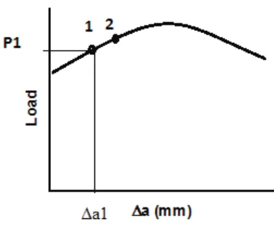
Fig. 1. Schematic Illustration of the FAD methodology

Fig. 2. Typical load vs. crack extension curve

*+,(- ) 4; < =>?,(@8A=>B < =>CDEF4%=>G,(H8I

(6)

Above equation for failure line is called option-1 curve which gives most conservative assessment. *+,₍-'is plotted up to maximum ,',₍ called ,_(12J', which is defined as,

,_(12J )4567< 5K78 L

(7)

Where 5_K7 is ultimate tensile strength of the material.

This can be rewritten as following,

$123) $9M*+,(-NO@

(8)

where, $₉ ) !_.@RPQ, where PQ ) P for plain stress while P +; % SR @- for plain strain case. Similarly,

$123 ) !123@RPQ is assumed.

Using Eqn. (8), fracture toughness, $₁₂₃ can be calculated for applied normalised loading ,₍ using FAD assessment line. This methodology is explained graphically in Fig. 1. Suppose we choose one assessment point corresponding to load point,1 beyond failure line (ductile crack initiation). Now, for getting''$₁₂₃, for loading 1, the assessment point is moved vertically on FAD assessment line, *+,₍- which is shown as point 1’. A typical experimentally obtained load vs. crack extension curve is shown in Fig. 2. At loading point 1, the total crack size 0_T, used for calculation will be 0_T) 0_U<$0_T, where 0_U'is initial crack size and $0_T is the instantaneous crack extension as shown in Fig. 2. For this loading point, values of !_.+"_T/ 0_T- and

(4)

EXPERIMENTAL RESULTS

Geometric and loading details

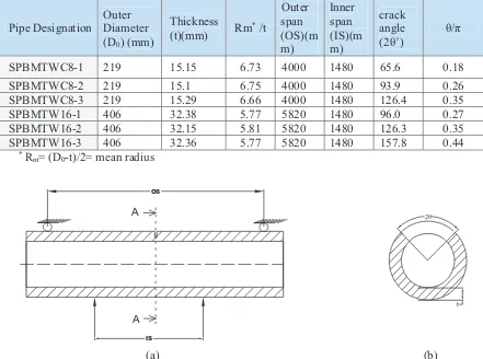
A comprehensive Component Integrity Test Program was initiated by Bhabha Atomic Research Centre (BARC), India in 1998. Under this program, large numbers of straight pipes were tested by Chattopadhyay et.al. (2000) and Chattopadhyay et.al. (2006). Important aspects of those fracture tests on pipes are revisited here. In this program, four point bending moment were applied quasi-statically during test. All straight pipes have been fabricated with throughwall circumferential cracks of different sizes. In this study we have chosen total 6 straight pipes; 3 numbers of both 8 inch and 16inch nominal diameter sizes. Relevant dimensions of pipes are shown in Table 1.The loading configuration is shown in schematic diagram in Fig. 3(a) and corresponding crack configuration is shown in Fig. 3(b). All pipes have been fatigue precracked to produce very sharp crack from machined crack. A static and monotonic load is applied on the pipe specimens under displacement control. Different instrumentations are mounted on test configurations for monitoring and recording different experimental results like total applied load, crack growth, displacements, etc.

Table 1: Dimensions of pipes with circumferential cracks.

Pipe Designation

Outer Diameter (D0) (mm)

Thickness (t)(mm) Rm

*_/t

Outer span (OS)(m m)

Inner span (IS)(m m)

crack angle (2!_û₎

!_/"

SPBMTWC8-1 219 15.15 6.73 4000 1480 65.6 0.18

SPBMTWC8-2 219 15.1 6.75 4000 1480 93.9 0.26

SPBMTWC8-3 219 15.29 6.66 4000 1480 126.4 0.35

SPBMTW16-1 406 32.38 5.77 5820 1480 96.0 0.27

SPBMTW16-2 406 32.15 5.81 5820 1480 126.3 0.35

SPBMTW16-3 406 32.36 5.77 5820 1480 157.8 0.44

* _R

m= (D0-t)/2= mean radius

A

A OS

IS

t %&

(a) (b)

(5)

Material Properties

Materials properties have been obtained from standard tensile tests and three-point bend (TPB) specimens for the SA 333 Grade 6 carbon steel used in the pipe tests as discussed by Chattopadhyay et.al. (2000). Results are presented in Table 2; the yield stress,'5_67', ultimate stress, 5_K, and fracture toughness data depend on the outer diameter of the pipe, Do. Ductile initiation fracture toughness values J0.2 were obtained

using stretch zone width (SZW) measurements at a crack growth of $0 =0.2mm.

Table 2: Properties of SA 333 Grade 6 steel as a function of pipe diameter

D0 [mm]! E [GPa]! '' #ys [MPa]! #u [MPa]! J0.2 [N/mm]!

219 203 0.3 288 420 220

406! 203! 0.3 312 459 236

For the 219mm pipe diameter, initiation toughness was determined from TPB 8 specimens with a relative crack depth a/W=0.513 and for the 406mm pipe from TPB 16 specimens with a/W=0.453.

CLOSED FORM EXPRESSIONS

Stress intensity factor, KI,

In order to apply FAD methods, it is necessary to evaluate the stress intensity factor, K . The following I

solution for circumferentially through-wall cracked pipes under in-plane bending moment [R6 (2013) and Zahoor, A. (1985)] was used:

a F

K_I) _b#_b (

(9)

where the bending stress, #_b, is defined in terms of the bending moment M as _b

) t R /(

M_b 2_m

b ) (

#

(10)

The correction function, F , in Eqn.(9) is _b

*

+

*

+

,

1.5 4.24

-b 1 A4.5967 / 2.6422 /

F ) . & ( . & ( 'VWX'

55 . 0 / 00& (/

(11)

where

*

+

,

-

0.25 m/t 0.25

R 125 . 0

A) 1 'VWX'5/Rm/t/10

(12)

For each pipe the values of the ratios Rm/t and &/( are included in Table 1. All the pipes tested are within the validity limits on R_m/t and &/( in Eqns. (11) and (12).

Limit Load, PL

(6)

Y#) Z&1@[\]567

(13)

Where,

\] ) *]+!- ^_` a % =>?*b+!- ^_` c

(14)

Where,

*]+!- ) ; <!@R;L , *b+!- ) ; <!@RG, a ) +d % c- LR and ''!) [ &R 1

R-6 CALCULATION

Procedure

The experimental load vs. crack extension data is converted to J-R curve using R-6 failure assessment method. In this paper option-1 failure assessment line of R-6 method is used in all calculations because it

is the most conservative and represented by a unique equation (Eqn.(6) ). Using the Eqn. (9), stress intensity factor is calculated for the pipe for the prevalent crack size and other geometry parameters for

any arbitrary loading, P and instantaneous total crack size, 0. Subsequently, $₉ is calculated using the relation''$₉ ) !_.@RPQ, where PQ ) P assuming plain stress case because of lower thickness of pipes. Limit

moment,'Y_#, is calculated using the Eqn. (13), where, 5₆₇'is yield stress of the relevant size of pipe, which is taken from Table 2. Limit moment is converted to limit load based on the loading configuration

of pipe as shown in Fig. 3(a) and can be written mathematically as,

"#)_{+ef % gf-}ZY#

(15)

The values of Outer Span (OS) and Inner Span (IS) can be obtained from Table 1. Normalized applied loading, ,₍ is calculated using Eqn. (3). Then, using Eqns.(6) and (8), $₁₂₃' is calculated for this arbitrary loading, P and crack size,''0. For other loading points, this procedure is repeated and consequently, entire J-R curve is obtained.

Results

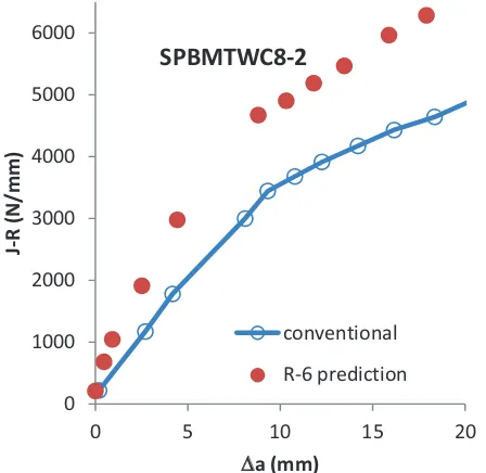
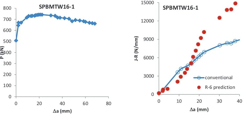
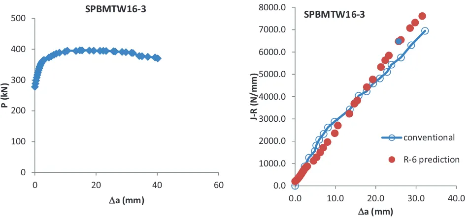
Using experimental load vs. crack extension data, J-R curves for all pipes are calculated using R-6 method and shown for all pipes from Fig. 4 to Fig. 9. It can be observed that for SPBMTWC8-1, R-6 J-R curve is showing good agreement with conventionally computed that one as shown in Fig. 4. However, For SPBMTWC8-2 and SPBMTWC8-3 pipes, R-6 methodology are over predicting the J-R curves than conventional approach especially for higher loadings as depicted in Fig. 5 and Fig. 6. For 16 inch pipes, the J-R curves calculated by both approaches are reasonably in good agreements as shown in Fig. 7, Fig. 8 and Fig. 9. Basically, the validity limit for R-6 approach is that the normalized applied loading, ,₍ h ; i.e.

5(9: h 56. In other words, the loading should be in the regime of small scale yielding. Assumption of global elastic deformation is also essential because we are using the relation, '$ ) !_.@RPQ for the derivation of Eqn. (8). Variation of ,₍' is shown in Fig. 10 for all pipes with respect to extended cracks. It can be observed that normalized loadings,'',₍s ,are closer to validity limits for 16 inch pipes than 8 inch pipes. Thus, the results are in good agreements for 16 inch pipes compare to 8 inch pipes.

(7)

(a)Experimental load vs. crack extension plot (b) R-6 prediction is compared with conventional

Fig. 4. Results of pipe SPBMTW8C-1.

(a) Experimental load vs. crack extension plot (b) R-6 prediction is compared with conventional

Fig. 5. Results of pipe SPBMTW8C-2.

0 50 100 150 200 250 300

0 20 40 60 80

P

!

(k

N

)

$a!(mm)

SPBMTWC8

_"

1

0 2000 4000 6000 8000

0 10 20 30 40

J

"

R

!

(N

/m

m

)

$a_!(mm)

SPBMTWC8

_"

1

conventional R!6"prediction

0 50 100 150 200 250

0 20 40 60 80

P

!

(k

N

)

$a!(mm)

SPBMTWC8

_"

2

0 1000 2000 3000 4000 5000 6000

0 5 10 15 20

J

"

R

!

(N

/m

m

)

$a_!(mm)

SPBMTWC8

_"

2

conventional

(8)

Fig. 6. Results of pipe SPBMTWC8-3.

Fig. 7. Results of pipe SPBMTWC16-1

0 20 40 60 80 100 120 140 160

0 20 40 60

P

!

(k

N

)

$a_!(mm)

SPBMTWC8

_"

3

0 1000 2000 3000 4000 5000 6000

0 5 10 15 20

J " R ! (N /m m )

$a!(mm)

SPBMTWC8

_"

3

conventional

R!6"prediction

0 100 200 300 400 500 600 700 800

0 20 40 60 80

P

!

(k

N

)

$a_!(mm)

SPBMTW16

_"

1

0 3000 6000 9000 12000 15000

0 10 20 30 40

J " R ! (N /m m )

$a_!(mm)

SPBMTW16

_"

1

conventional

(9)

0 100 200 300 400 500 600 700

0 20 40 60 80

P

!

(k

N

)

$a!(mm)

SPBMTW16

_"

2

0 2000 4000 6000 8000

0.0 10.0 20.0 30.0

J

"

R

!

(N

/m

m

)

$a!(mm)

SPBMTW16

_"

2

conventional

R_!6_"prediction

0 100 200 300 400 500

0 20 40 60

P

!

(k

N

)

$a!(mm)

SPBMTW16"3

0.0 1000.0 2000.0 3000.0 4000.0 5000.0 6000.0 7000.0 8000.0

0.0 10.0 20.0 30.0 40.0

J

"

R

!

(N

/m

m

)

$a!(mm)

SPBMTW16"3

conventional

(10)

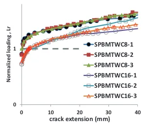
Fig. 10. Variations of normalized loadings, Lr

STRESS TRIAXIALITY RESUTLS

O’dowd and Shih (1991) introduced the non-dimensional parameter, ’Q’, to quantify the crack tip constraint. By this theory, the laboratory specimen must match the constraint of the component for transferability of fracture toughness property. Q is defined as,

i )A5jj% +5jj-(9:I

567 0[ c ) = % k=

l_/ _{m )} L$

567

(16)

where, r and & are polar co-ordinates with origin situated at the crack tip. #_&& is existing stress field ahead of the crack tip of the actual specimen or component, (#_&&₎_ref_{is reference solution obtained from standard}

plain strain small scale yielding solution (#_&&₎_SSY_{as explained by O’Dowd and Shih (1993).}

Three dimensional finite element analyses are carried out for all pipes, as explained by Chattopadhyay et.al (2000). The stress triaxiality parameter, Q, is dependent on applied loading and consequent crack driving force, J. Hence one specific loading point has to be chosen for comparing crack tip constraint. It is established that at crack initiation point the applied crack driving force is equal to J0.2 for TPB specimen for

respective pipes, which is established as a material property. For these materials, the reported value of J0.2

are 220N/mm and 236N/mm for 8 inch and 16 inch piping material [Tarafder et.al. (2000)] as shown in Table 2. Hence for all cases, the loading point chosen for computation of Q is corresponding to J-integral = J0.2 of related piping material. Crack opening stress and thus, stress triaxiality is the highest at the center

of the crack front for all pipes Hence, for getting conservative estimate, the stress triaxiality has been computed at the center of crack front. The crack opening stress is obtained at distance of cJ/#₀_{(where c =}

1, 2, 3, 4, 5) ahead of crack tip at &=0. The variation of stress triaxiality in the remaining ligament is depicted in Fig. 12. Based on these findings it can be stated that the crack tip constraints are higher for 16 inch pipes

0

1

0

10

20

30

40 N

o

rm

a

li

ze

d

!

lo

a

d

in

g

!

,

!

Lr

crack

_!

extension

_!

(mm)

SPBMTWC8

_"

1 SPBMTWC8

_"

2 SPBMTWC8

_"

3 SPBMTWC16

_"

1 SPBMTWC16

_"

2

(11)

than 8 inch pipes and crack tip constraints are significantly dependent on the size of pipes instead of present crack sizes.

Fig. 11. J-R curves are segregated based on the size of the pipes.

Fig. 12. Variation of Stress triaxiality parameter, Q on remaining ligament

CONCLUSION

A simple R6 based approach is proposed for evaluation of J-R curve from experimental load-crack growth data. It is utilized to calculate J-R curves of 8 and 16 inch diameter pipes with throughwall circumferential cracks under four point bending load. The J-R curves thus calculated are showing good agreement with conventionally calculated values especially for 16 inch pipes. It is found that 16 inch pipe J-R curves are lower than those of 8 inch pipes, which has been attributed to higher crack tip constraints for 16 inch pipes. An attempt has been made to explain the better matching of J-R curves for 16 inch pipes with conventional calculations. The drawback of this methodology is that it is based on single point experimental data unlike conventional approach, where entire history of load vs. displacement results is integrated. Thus, in the presently proposed method, error at arbitrary experimental data point will lead to significantly erroneous fracture toughness data.

REFERENCES

Rice J. R., Paris P. C., Merkle J. G. (1973). Some further results of J-integral analysis and estimates.” In: Progress in Flaw Growth and Fracture Toughness Testing, ASTM STP 536. Philadelphia: American Society for Testing and Materials; 231–45.

Ernst H. A, Paris P. C., Rossow M., Hutchinson J.W. (1979). Analysis of load displacement relation to determine J–R curve and tearing instability material properties. In: Smith CW, editor. Fracture Mechanics, ASTM STP 67. Philadelphia: American Society for Testing and Materials;. 581–99. Zahoor A., Kanninen M.F. (1981). A plastic fracture mechanics prediction of fracture instability in a

(12)

Chattopadhyay J., Dutta B. K., Kushwaha H. S. (2004). New ‘!p’ and ‘"’ functions to evaluate J-Rcurve from cracked pipes and elbows. Part I: theoretical derivation. Engineering Fracture Mechanics. 71, 2635-2660.

Gurson A. (1977). Continuum theory of ductile rupture by void nucleation and growth: Part-I: yield criteria and flow rules for porous ductile media. J. Engg. Mater. Technol. 99(1), 2-15.

Tvergaard V., Needleman A. (1984). Analysis of the cup-cone fracture in a round tensile bar. Acta. Metall. 32, 157-169.

Ainsworth, R. A. (2003), 7.03-Failure Assessment Diagram Methods, Comprehensive Structural Integrity, 7, 89-132.

Ainsworth R. A., Gintalas M., Sahu M. K., Chattopadhyay J., Dutta B. K. (under review). Application of Failure Assessment Diagram Methods to Cracked Straight Pipes and Elbows. Int. J. Pressure Vessels and Piping

Dowling A. R., Townley C. H. A. (1975). The effects of defects on structural failure: a two-criterion approach, In. J. Pressure Vessels Piping, 3, 77-107.

Harrison R. P., Loosemore K., Milne I. (1976). Assessment of the integrity of the structures containing defects. CEGB Report R-H-R6. UK: Central Electricity Generation Board.

Chattopadhyay J., Dutta B. K., Kushwaha H. S. (2000). Experimental and analytical study of three point bend specimen and throughwall circumferentially cracked straight pipe, Int. J. Pressure Vessels and Piping, 77, 455-471.

Chattopadhyay J., Kushwaha H. S., Roos E. (2006). Some recent developments on integrity assessment of pipes and elbows. Part II: Experimental investigations, Int. J. Solids and Structures. 43, 2932-2958. R6 (2013): Assessment of the integrity of structures containing defects, Revision 4, including subsequent

updates. EDF Energy Generation, Gloucester, UK.

Zahoor, A. (1985). Closed form expressions for fracture mechanics analysis of cracked pipes, ASME J Pres Ves Technology 107, 203-205.

Jones, M. R. and Eshelby J M (1990). Limit load solutions for circumferentially cracked cylinders under internal pressure and combined tension and bending. Nuclear Electric Report, TD/SID/REP/0032. O’Dowd N. P., Shih C. F. (1991). Family of crack tip fields characterized by a triaxiality parameter1I:

structure of fields, J Mech Phys Solids, 39, 898-1015.

O’Dowd N. P., Shih C. F. (1993). Two parameter fracture mechanics: theory and application, NUREG /CR-5958.