A Novel Approach for Software Defect Prediction Using Learning Algorithms

(1)

ISSN(Online): 2320-9801

ISSN (Print) : 2320-9798

I

nternational

J

ournal of

I

nnovative

R

esearch in

C

omputer

and

C

ommunication

E

ngineering

(A High Impact Factor, Monthly, Peer Reviewed Journal) Website: www.ijircce.com

Vol. 5, Issue 11, November 2017

A Novel Approach for Software Defect

Prediction Using Learning Algorithms

Maheswari S1, Chitra K2

Research Scholar, Bharathiyar University, Coimbatore, India1

Assistant Professor, Department of Computer Science, Government Arts College, Melur, India2

ABSTRACT: Software development is increasing rapidly. For a few reasons, the software brings many defects. In the development of software testing each module in the software is the main stage to reduce software defects. If the developer or testers can correctly predict software defects, you can reduce costs, time and effort. This paper shows a comparative study of existing methods in a prediction of software defects based on classification rules mining. We propose a method for this process and we select different classification algorithms. In this analysis we take historical datasets like NASA MDP dataset for prediction of performance in the software defects. The results of this method show that we comparing to proposed new algorithm with different algorithms according to the classification rule mining of different data sets.

KEYWORDS:Classifier, Confusion Matrix, Defect Prediction, Rule Mining, Software metrics.

I. INTRODUCTION

A.

Introduction to Software Defect Prediction:

In recent years, the demand for software quality has increased dramatically. As a outcome, issues are related to testing, becoming progressively more critical. The ability to measure software defects is more significant to minimize costs and improve the overall efficiency of the testing process. Few of software components are the reason of major amount of defects in the software system.

Knowing the causes of possible defects and determining the general software process areas that may need to be taken into description from the initialization scheme could save time and effort. The chance of premature estimating the possible defects of software could help on preparation, scheming and executing software development activities. The low-cost method of defect analysis is to learn from past mistakes to prevent future mistakes. Today, we can extract several datasets of data to find useful knowledge about defects.

Using this information should possibly be able to:

1. Identify potential software failures.

2. Estimate the unique number of defects and

3. Find out the possible causes of software defects.

B. Objective

Taking the signs of the investigation, there has been sufficient scope to improve the prediction of software defects.

The objectives of this research are summarized to the following:

 To efficiently remove the noise in the novel dataset using latest filtering mechanism.

 To create novel algorithm to predict software defects.

 Using efficient classification algorithm for better prediction of software defects.

 Using efficient metrics and methods to evaluate the result.

 To create low-cost software development.

(2)

ISSN(Online): 2320-9801

ISSN (Print) : 2320-9798

I

nternational

J

ournal of

I

nnovative

R

esearch in

C

omputer

and

C

ommunication

E

ngineering

II. BACKGROUND & LITERATURE SURVEY

A. Data Mining for Software Engineering:

In order to improve productivity and software quality, software engineers are applying data mining algorithms to a variety of software engineering tasks. Many algorithms can help engineers understand how to call API methods provided by libraries or complex frameworks, and the documentation is inadequate. In terms of maintenance, these types of data mining algorithms can helps to determine which code locations should be changed when changing other code locations. The software engineer can also use the data mining algorithms to find possible defects that may cause future failures on the site and identify lines of code (LOC) errors that are responsible for known faults.

B. Software defect predictor

Defect predictors are tools or methods that guide test activities and software development lifecycles. According to Brooks, half of the software development costs are in unit and system testing. Harold and Tahat also believe that the testing phase requires about 50% or more of the entire project progress. Thus, the main challenge is the testing phase where professionals are looking for predictors that indicate possible defects before the test begins. This can effectively allocate them for limited resources. The defect prediction factors are used to order modules that are verified by verification and validation teams:

 If do not have enough resources to check the entire code, defect predictors can be used to increase the chances

of being checked for defects.

 If check the entire code, but the inspection process will take several weeks or months to complete, you can use

the defect predictors to improve the possibility that the error module will be checked in advance. This is useful because it allows the development team to inform which modules need rework early, so it gives more time to complete the review before delivery.

C. Related Works

Regression via classification

In 2006, Bibi, Tsoumakas, Stamelos, Vlahavas, applied the machine learning method to estimate the number of defects that were referred to as the classification of the route classification (RFC) [4]. The whole process by classification (RFC) regression involves two important steps:

 Discrete numerical variables to learn the classification model,

 In the inverse process of a numerical prediction model transformation class output.

Static Code Attribute

Menzies, Greenwald and Frank (FGM) [5] published a study in the journal 2007 comparing two machine learning techniques (the rules incorporate naive Bayesian) performance prediction of defective software components. To do this, they use the library MDP NASA, which, during the survey, contains 10 separate data sets.

ANN

In 2007, Casi Gondra [6] used to predict defective machine learning methods. He uses artificial neural networks as apprenticeships.

Embedded software defect prediction

In 2007, oral. And Bender [7] used Multi-Layer Perceptron (MLP), NB, VFI (Voting Function Interval) for embedded software defect prediction. It has been used to evaluate only 7 datasets.

Association rule classification

In 2011, Pojun Karel [3] used a CBA2-based rule-based association for predicting software defect classification. Classification of association rules used in these surveys. And they compared to the other classification rules C4.5 and the Ripper.

Defect-proneness Prediction framework

In 2011, Song Jia, Liu Yinghe proposed a software framework for predicting the tendency to defects. In this study, the learning process of M * N cross-validated data sets (NASA, Softlab dataset) was used. They used three classification algorithms (Naive Bayes and OneR, J48), and compared with the FGM framework [5].

(3)

ISSN(Online): 2320-9801

ISSN (Print) : 2320-9798

I

nternational

J

ournal of

I

nnovative

R

esearch in

C

omputer

and

C

ommunication

E

ngineering

III. PROPOSED SCHEME

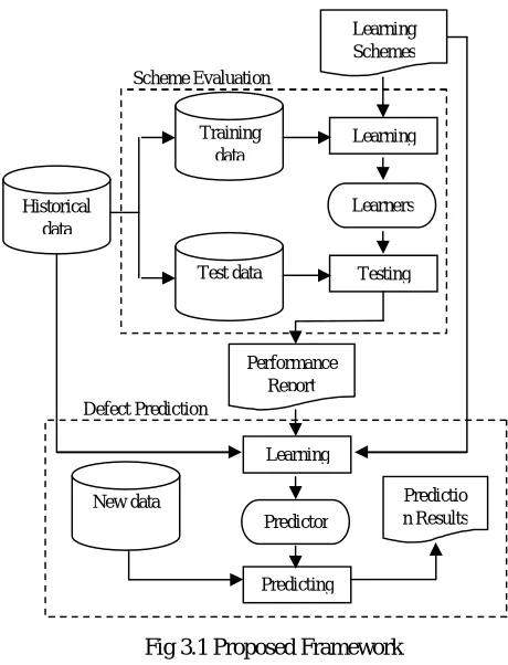
A. Overview of the Framework

Before creating a prediction model for defects and using it for the purpose of forecasting, we must first determine what apprenticeship or learning algorithm should be used to build the model. Thus, the predictive performance of the apprenticeship program should be determined, especially for future data. However, this step is often overlooked, so the resulting prediction model can be unreliable. As a result, we use outline for prediction of software defects to provide guidance to address these potential defects

The framework consists of two parts:

1) Scheme evaluation and

2) Defect prediction.

The details contained in Figure 3.1. During the evaluation phase of the program, the results of the historical data of the different learning programs are evaluated to determine whether the learning program is not good enough to predict the purpose or to select the best group of competing programs.

In Figure 3.1, we can see that the historical data is divided into two parts:

Fig 3.1 Proposed Framework

Based on the report of the first-level performance, the learning scheme is selected and used to establish the prediction model and predict the software defects. Figure 3.1, we note that all the historical data come here to build the forecast. This is very different from the first level; it is very useful to improve the generalization ability of the forecast. Once a new software component is forecasted that can be used to predict the tendency to be flawed.

MGF presented [5] a controlled experiment and reported the excavation of naive Bayesian data with log filter performance and attribute selection, which was carried out with the appropriate data to be evaluated. This is because they use two training data (which can be regarded as historical data) and tests (which can be considered as new data) to classify the attributes, while the tag new data is not provided to the selection of the attributes in practice.

Scheme Evaluation

Defect Prediction

New data

Learning

Predicting Predictor

Predictio n Results Historical

data

Training data

Test data

Learning

Testing Learners

Performance Report

(4)

ISSN(Online): 2320-9801

ISSN (Print) : 2320-9798

I

nternational

J

ournal of

I

nnovative

R

esearch in

C

omputer

and

C

ommunication

E

ngineering

B. Scheme Evaluation

The evaluation program is an important part of the framework for software defect prediction. At this stage, different learning programs are evaluated and built with them to test the learners. The first question of the evaluation of the program is how to divide historical data into training and testing. As described above, the test data must be independent of the pupil's configuration. It is necessary to assess the performance of new data for learners' prerequisites. Cross validation is generally used to estimate the accuracy of the work with the actual prediction model. The circular cross validation involves the compilation of data into complementary subsets that perform analysis in other subsets of analysis and validation of a subset. In order to reduce variability, multiple rounds of cross validation were performed using different partitions, and the results were validated in two rounds.

In our framework, we used to estimate the proportion of the performance of each prediction model, that is, each data set is first divided into two parts, after which the lessons are predicted in 60% of the cases, and then the remaining 40% of the test.

In order to overcome any impact of management and obtain reliable statistical data, each experimental residual molecule also repeats M times and is repeated at each iteration of the data set. Thus, in general, the model M * N (N = data set) is constructed during the total evaluation period; and M * N results are obtained for each learning pattern of performance data in each group.

After the split training test each round is both training data and learning mode (S) for building a student. The learning scheme is data preprocessing, a method of selecting method properties and learning algorithms.

1. A data preprocessor

 Training data for preprocessing, such as eliminating outliers, missing numerical discrepancies or

attribute values processing and processing.

 The preprocessor is used here - the NASA preprocessing tool

2. An attribute selector

 We considered the MDP data from all the attributes provided by NASA.

C. Scheme Evaluation Algorithm

Data: Historical Data Set

Result: The mean performance values Step 1: M=12 :No of Data Set Step 2: i=1;

Step 3: while i<=M do

Step 4: Read Historical Data Set D[i]; Step 5: Split Data set Intances using % split; Step 6: Train[i]=60% of D; % Training Data; Step 7: Learning(Train[i],scheme);

Step 8: Test Data=D[i]-Train[i];% Test Data; Step 9: Result=TestClassi_er(Test[i],Learner); Step 10: end

Algorithm 1: Scheme Evaluation D. Defect prediction

Predicting the defects of our framework is simple; it includes forecasting and predicting construction deficiencies. During the construction period:

1. The learning program is selected as a work report.

2. A prediction is structured as having a selected learning plan and complete historical data. When evaluating a

planned study, the student is established with test data from the test and test data. His final performance is averaged in every round. The assessment shows that the effective coverage of all the data. So, using all the historical data to build the forecast, it is expected to have a larger capacity for the built-in forecast for larger capacity.

3. Once the forecast is established and the new data is in the same way as historical data, the built-in predictions

(5)

ISSN(Online): 2320-9801

ISSN (Print) : 2320-9798

I

nternational

J

ournal of

I

nnovative

R

esearch in

C

omputer

and

C

ommunication

E

ngineering

E. Difference between Our Framework and Others

So, to summarize the main differences between our framework and others in the following:

1) We choose all the learning plans, not just out of the learning algorithm, attribute selector or data preprocessing

unit;

2) We use the appropriate mechanism to assess the performance of the data architecture. | -NASA set MDP [9]

data.

3) We selected the training data set (60%) and the test data set (40%) percentage split.

F. Data Set

4) We use data from the public repository NASA MDP, which also uses MGF and many other countries, for

example, [10], [11], [12], [13]. Therefore, a total of NASA MDP 12 data sets.

5) Table 3.1 and 3.2 Basic profile information are provided. Each data set consists of a series of software

modules (examples), each of which contains defects and several attributes of static software code corresponding to the number. After preprocessing, the module contains one or more defects marked as faulty.

6) A more detailed description of the attributes of the source code or MDP dataset is available from [5].

Table 3.1 NASA MDP Data Sets

Dataset System Language Total Loc

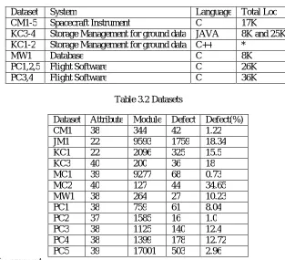
CM1-5 Spacecraft Instrument C 17K

KC3-4 Storage Management for ground data JAVA 8K and 25K

KC1-2 Storage Management for ground data C++ *

MW1 Database C 8K

PC1,2,5 Flight Software C 26K

PC3,4 Flight Software C 36K

Table 3.2 Datasets

Dataset Attribute Module Defect Defect(%)

CM1 38 344 42 1.22

JM1 22 9593 1759 18.34

KC1 22 2096 325 15.5

KC3 40 200 36 18

MC1 39 9277 68 0.73

MC2 40 127 44 34.65

MW1 38 264 27 10.23

PC1 38 759 61 8.04

PC2 37 1585 16 1.0

PC3 38 1125 140 12.4

PC4 38 1399 178 12.72

PC5 39 17001 503 2.96

G. Performance Measurement

(6)

ISSN(Online): 2320-9801

ISSN (Print) : 2320-9798

I

nternational

J

ournal of

I

nnovative

R

esearch in

C

omputer

and

C

ommunication

E

ngineering

Table 3.3 Confusion Matrix

Predicted Class

Actual Class

Positive Negative

Positive True Positive False Negative

Negative False Positive True Negative The proposed program software defects are based on the accuracy of the prediction,

Sensitivity, Specificity, Balance Area defined as:

Accuracy=

Sensitivity=

Specificity =

IV. RESULTS AND DISCUSSION

This section provides some simulation results from the so-called MATLAB (version 2009a) simulation software tool to compile the classification algorithm. The proposed work is further compared with the appropriate scheme.

According to the best precision values, we have chosen one of the ranking algorithms 8 for many classification algorithms. All the evaluation values, and compares them with different parameter performance measurements.

A. Accuracy

From the precision table 4.1, we can see different algorithms that allow different precision in different datasets. But the average yield is almost the same. Storage management software (KC1-3) LOG, J48G provides a better precision value. For the C programming language (MW1) database software only part of the application of higher precision values

Table 4.1 Accuracy

Methods NB LOG DT JRip OneR PART J48 J48G Proposed

CM1 83.94 87.68 89.13 86.23 89.13 73.91 86.23 86.96 89.13

JM1 81.28 82.02 81.57 81.42 79.67 81.13 79.8 79.83 83.04

KC1 83.05 86.87 84.84 84.84 83.29 83.89 85.56 85.56 87.91

KC3 77.5 71.25 75 76.25 71.25 81.25 80 82.5 84.8

MC1 99.34 99.27 99.25 99.22 99.3 99.19 99.3 99.3 99.34

MC2 66 66.67 56.86 56.86 56.86 70.59 52.94 54.9 69.23

MW1 79.25 77.36 85.85 86.79 85.85 88.68 85.85 85.85 89.14

PC1 88.82 92.11 92.43 89.14 91.45 89.48 87.83 88.49 89.62

PC2 94.29 99.05 99.37 99.21 99.37 99.37 98.9 98.9 99.37

PC3 84.38 84.67 80.22 82.89 82.89 82.67 82.22 83.56 84.02

PC4 87.14 91.79 90.18 90.36 90.18 88.21 88.21 88.93 92.27

(7)

ISSN(Online): 2320-9801

ISSN (Print) : 2320-9798

I

nternational

J

ournal of

I

nnovative

R

esearch in

C

omputer

and

C

ommunication

E

ngineering

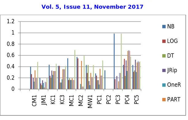
B. Sensitivity

Precision Table 4.2, we see, NB provides the largest set of data to perform better algorithms. For Decision Table gives zero sensitivity (sometimes), which means that the whole class is considered true. LOG and OneR part, J48, J48G gives the average rate of return.

Table 4.2 Sensitivity

CM1 0.4 0.267 0 0.2 0.133 0.333 0.2 0.2 0.483

JM1 0.198 0.102 0.07 0.157 0.109 0.03 0.131 0.123 0.198

KC1 0.434 0.238 0.197 0.328 0.254 0.32 0.32 0.32 0.450

KC3 0.412 0.412 0.118 0.118 0.176 0.353 0.353 0.353 0.412

MC1 0.548 0.161 0.194 0.161 0.161 0.194 0.161 0.161 0.693

MC2 0.572 0.545 0 0 0.091 0.5 0.045 0.045 0.591

MW1 0.429 0.286 0.429 0.143 0.071 0.286 0.214 0.214 0.429

PC1 0.28 0.24 0.16 0.16 0.08 0.36 0.24 0.24 0.51

PC2 0.333 0 0 0 0 0 0 0 0

PC3 0.986 0.178 0 0.233 0.014 0.137 0.288 0.288 0.986

PC4 0.431 0.538 0.231 0.508 0.323 0.677 0.692 0.677 0.577

PC5 0.427 0.308 0.332 0.521 0.303 0.474 0.498 0.479 0.491

0 20 40 60 80 100 120

C

M

1

JM

1

K

C

1

K

C

3

M

C

1

M

C

2

M

W

1

P

C

1

P

C

2

P

C

3

P

C

4

P

C

5

NB

LOG

DT

JRip

OneR

(8)

ISSN(Online): 2320-9801

ISSN (Print) : 2320-9798

I

nternational

J

ournal of

I

nnovative

R

esearch in

C

omputer

and

C

ommunication

E

ngineering

C. Specificity

From the specific form, we can see some algorithms that allow 100% of the specificity and cannot be regarded as their respective zero sensitivity. These algorithms can give incorrect predictions. According to the sensitivity and specificity, because they give 100%, but 0% of the sensitivity of the high specificity of the algorithm should not consider Decision Table prediction software defects.

Table 4.3 Specificity

CM1 0.893 0.951 1 0.943 0.984 0.789 0.943 0.951 0.986

JM1 0.956 0.988 0.99 0.968 0.957 0.994 0.954 0.956 0.956

KC1 0.898 0.976 0.959 0.937 0.932 0.927 0.947 0.947 0.983

KC3 0.873 0.794 0.921 0.937 0.857 0.937 0.921 0.952 0.922

MC1 0.947 1 0.999 0.999 1 0.999 1 1 1

MC2 0.724 0.759 1 1 0.931 0.862 0.897 0.931 1

MW1 0.848 0.848 0.924 0.978 0.978 0.978 0.957 0.957 0.978

PC1 0.943 0.982 0.993 0.957 0.989 0.946 0.935 0.943 0.999

PC2 0.946 0.997 1 0.998 1 1 0.995 0.995 1

PC3 0.219 0.976 0.958 0.944 0.987 0.96 0.926 0.942 0.966

PC4 0.929 0.968 0.99 0.956 0.978 0.909 0.907 0.917 0.928

PC5 0.983 0.99 0.991 0.987 0.99 0.985 0.986 0.987 0.990

0 0.2 0.4 0.6 0.8 1 1.2

C

M

1

JM

1

K

C

1

K

C

3

M

C

1

M

C

2

M

W

1

P

C

1

P

C

2

P

C

3

P

C

4

P

C

5

NB

LOG

DT

JRip

OneR

(9)

ISSN(Online): 2320-9801

ISSN (Print) : 2320-9798

I

nternational

J

ournal of

I

nnovative

R

esearch in

C

omputer

and

C

ommunication

E

ngineering

D. Comparison with other's results

• In 2011, Song Jia, Liu Ying and put forward a general framework. In this respect, they use the OneR algorithm for predicting defects, but should not be considered as a drawback for prediction because it gives 0 times the sensitivity and balance values smaller than others.

• FGM used 10 datasets in 2007, and our study used 12 sets of data for more data in each module. And our result is that the balance sheet value is also higher than the effect.

• In different learning algorithms and other works used in the machine. In our study, the results of the comparative measurements were increased. Because we use the division ratio is mainly to improve the accuracy.

V. CONCLUSION

In our study, we tried to solve the problem of software defect prediction (classification) in different data mining algorithms. Proposed algorithm give predictive flaws the best overall performance and offers better performance than OneR and JRip. From these results, we saw that a preprocessing selection / attribute data can be used with different learning algorithms for different datasets, and no apprenticeships dominate, that play a different role, always outperforming all other data sets. This means that we have to choose different data sets for different learning programs, so the assessment and decision making process is very important.

REFERENCES

1. Tao xie, Suresh Thummalapenta, David Lo, and Chao Liu.Data mining for Software Engineering .computer ,42(8):55-62, 2009.

2. Oinbao Song, Zihan Jia , Martin Shepperd, Shi Ying, and Jin Liu. A genera l software defect - proneness prediction framework. Software Engineering, IEEE Transactions on, 37(3):356-370, 2011.

3. Ma Baojun, Karel Dejaege,r Jan Vanthienen, and Bart Baesens .Software defect prediction based on association rule classification. Available at SSRN 1785381, 2011.

4. S Bibi G Tsoumakas, I stamelos, and I Vlahayas .software defect prediction using regression via classification, In IEEE International Conference on,pages 330-336,2006.

5. Tim Meenzies, Jeremy Greenwald,and Art Frank, Data mining static code attributesto learndefect predictors. Software Engineering, IEEE Transactions On,33(1):2-13,2007.

6. IkerGondra, Applying Machine Learning to software fault-proneness prediction. Journal of Systems and Software, 81(2):186-195, 2008. 7. Atac Deniz Oral and Ayse Basar Bener. Defect prediction for embedded software.In Computer and Information Sciences, 2007. iscis 2007. 22nd

International Symposium on, pages 1-6. IEEE,2007.

8. Yuan Chen, Xiang-heng Shen, Peng Du, and Bing Ge.Research on software defect prediction based on data mining. In Computer and Automation Engineering (ICCAE), 2010 .The 2nd_{International Conference on, volume 1, pages 563-567.IEEE, 2010.}

9. Martin Shepperd, Qinbao Song, Zhongbin.Sun, and Carolyn Mair. Data quality: Some comments on the nasa software defect data sets. 2013.

10. Stefan Lessmann Bart Baesens, Christophe Mues, and Swantje Pietsch Bench marking classification models for software defect prediction: A

proposed framework and novels findings, Software Engineering, IEEE Transaction on,34(4):485496,2008.

11. Yue Jiang, Bojan Cukic,and Tim Menzies.Fault prediction using early lifecycle data. In Software Reliability,2007. ISSRE’07 The 18th International Symposium on,pages 237-246.IEEE,2007.

(10)

ISSN(Online): 2320-9801

ISSN (Print) : 2320-9798

I

nternational

J

ournal of

I

nnovative

R

esearch in

C

omputer

and

C

ommunication

E

ngineering

12. Yue Jiang, Bojan Cuki , Tim Menzies, and Nick Bartlow, Companing design and code metrics for software quality prediction.In proceedings of the 4th_{international workshop on predictor models in software engineering, pages 11-18.ACM, 2008.}

13. Hongyu Zhang, Xiuzhen Zhang, and Ming Gu.Predicting defective software components from code complexity measures.In Dependable Computing, 2007. PRDC2007.13th Pacific Rim International Symposium on,pages 93-96.IEEE, 2007.

14. Gustavo EAPA Batista, Ronaldo C Prati,n and Maria Carolina Monard. A study nof the behavior of several methods for balancing machine learning training data.ACM SIGKDD Explorations Newsletter, 6(1): 20- 29, 2009.

15. Charles E Metz,Bejamin A herman, and Jon-Her Shen. Maximum likehood estimation of receiver operating characteristic (roc) curves from continuously- distributed data. Statistics in medicine, 17(9):1033-1053, 1998.

16. Oinbao Song,Martin Sheppered, Michelle Cartwright, and Carolyn Mair, Software defect, association mining and defect correction effort prediction models. Software engineering, IEEE Transactions On, 32(2):69-82, 2006.

17. Norman,.F.Fenton and Martin Neil. A critique of software defect prediction models.Software Engineering,IEEE Transactions on, 25(5):675-689,1999.

18. Naeem Seliya and Taghi M Khoshgoftaar software quality estimation with limited fauit data:a semi-supervised learning perspective. Software quality journal, 15(3):327-344, 2007.

19. Frank Padberg Thomas Ragg and Ralf Schoknecht Using machine learning for estimating the defect content after an inspection Software Engineering, IEEE Transactions on, 30(1):17-28, 2004.

20. Venkata UB Challagulla,Farokh B Bastani I- Ling Yen and Raymond A Paul Empirical assessment of machine learning based software defect

prediction techniques. In object- oriented real-time Dependable systems, 2005, WORDS 2005, 10th_{IEEE International Workshop on, Pages}