EECA Routing Protocol for FANETs

(1)

Vol. 4, Issue 3, March 2016

EECA Routing Protocol for FANETs

Rishab Sinha1, Vikash Kumar2, Nishi Yadav3

B.Tech VIII Semester, Dept. of Computer Science & Engineering, Central University, ITGGV, Bilaspur, Chhattisgarh, India1,2

Assistant Professor, Dept. of Computer Science & Engineering, Central University, ITGGV, Bilaspur, Chhattisgarh, India3

ABSTRACT: The usage of Unmanned Aerial Vehicles (UAVs) is increasing day by day. In recent years, UAVs are being used in increasing number of civil applications, such as policing, fire- fighting etc in addition to military applications. Instead of using one large UAV, multiple UAVs are nowadays used for higher coverage area and accuracy. Therefore, networking models are required to allow two or more UAV nodes to communicate directly or via relay node(s). Flying Ad-Hoc Networks (FANETs) are formed which is basically an ad hoc network for UAVs. In this paper, we have done a detailed study on some of the routing protocols of Flying Ad hoc Network and then, we have proposed a dynamic, distributed and hierarchal routing protocol EECA with increased energy efficiency and reduced number of transmission. The simulation results are shown under realistic conditions.

KEYWORDS: UAV; FANET; EECA; MPR; PBO; MANET

I. INTRODUCTION

Wireless Ad-hoc networks [1] are a collection of two or more devices equipped with wireless communication and network capabilities. It is an infrastructure-less or multi-hop network without any base stations. The use of large number of tiny, low power, low cost sensor nodes that have the ability of sensing the environment, processing the data and communicating with other nodes to form sensor networks [2]. In this scientific world, with the advent of new technologies in the field of sensor networks, It is ountpossible to create long range Unmanned Air Vehicles (UAV) [3], [4] systems which can fly independently without carrying any human on it and controlled remotely. The flexibility, ease of installation and relatively small operating expenses, enhanced usage of UAVs have many real world military applications like destroy operations, border surveillance as well as civilian applications like traffic monitoring and disaster management. Flying Ad-hoc Networks (FANETs) [5] are a special case of mobile ad-hoc networks (MANETs) which are characterized by a high degree of mobility. FANETs are actually ad-hoc network of multi-UAVs. The capability of a single UAV is limited. The coordination and collaboration of multiple UAVs can create a system that is beyond the capability of only one UAV.Some of the advantages of multi-UAV system over Single-UAV system are:-

 Cost: The cost expense of maintenance and acquisition of a single Large UAV is more than the cost of small UAVs.

 Range: The range of a single UAV is much smaller than a multi UAV system.

 Faster: The mission can be completed faster in Multi-UAV system than in Single-UAV.

 Failure recovery: If the single UAV goes down during the mission, It will lead to failure of the mission while in multi UAV other UAVs can go on to complete the mission.

Though it has a lot of advantages, FANET faces a lot of challenges. Some of the issues faced by FANETs are:-

 Node Density: FANET nodes are generally scattered and hence having low density of nodes.

 Topology Change: Topology change is quite frequent in FANET due to high speed of UAVs.

 Geographical challenges: Due to difference in weather in sky, UAVs are to be design in such a way so that it can be utilized in tough conditions.

 Routing challenges: Due to high speed, frequent topology change and different obstacles in sky, the routing algorithms needed for the communication between UAVs should be extensively accurate.

Routing is the center stage of the whole research paper. Routing algorithm is actually a way to find the shortest path from source to destination. Many topological routing algorithm has been designed viz.: -

A. Dynamic Source Routing: -

(2)

route cache. If a route is found it sends the packet through the route. If no route is found it broadcasts a route request with a unique identifier with respect to the route requests recently sent before from this node to the nodes in its direct radio transmission range in the network. In case a receiving node has seen a route request from the source with the same identifier before; it discards the route request, otherwise if it is the target of the route request, it sends a route reply with the passed nodes, otherwise, it looks for a route to the target of the route request in its route cache and sends a route reply with the route if found, if not found, it appends its address to the passed nodes in the route request and re-broadcasts the route request to the surrounding nodes in its direct radio transmission range till the destination is reached and the route to destination is returned.

B. Optimized Link State Routing: -

It is a proactive routing algorithm i.e. it maintains a table for the topological information by continuous periodic exchange of messages. It is an optimization of Link State Routing Algorithm as it reduces the size of message as well as reduces the number of transmissions to flood these messages in the entire network by using multi-point relays. C. Clustering Algorithm: -

This algorithm organizes nodes into groups called clusters [7]. Among these set of nodes, a particular node is selected as Cluster Head which has more proximity to the sink and is more energy efficient. The nodes who desire to send data packets to the sink transfers the data packets to the Cluster Head which then transmits the data to sink. D. Data Centric Routing: -

All the algorithms explained above are address centric routing algorithms which finds shortest path between addressable end nodes while Data Centric Routing which finds routes from multiple source to a particular destination that allows in-network consolidation of redundant data. It is actually a geographic hash table for data transfer.

In this paper, we are going to propose a new protocol for routing in FANETs by using data centric routing which is more energy efficient than address centric routing in cluster networks thus decreasing the cumulative energy of the network and hence a better prospect for the selection of cluster head and decreasing the total number of transmissions in the network.

II. RELATED WORK

A. Dynamic Source Routing: -

Dynamic Source Routing [6] is a reactive approach of routing in ad-hoc networks in which sending nodes recover the routes whenever they need to send data to the receiver nodes. Dynamic Source routing Algorithm is divided into two parts:

-Step 1: Route Discovery: -

In DSR, if the sender wants to send a data it checks in its route caches if the route [9] exists to the destination from source, the sender sends the data to the receiver through the path. Now, if the route doesn’t exist it broadcasts an initiator packet to all its neighbour nodes and if the node has received the same request before, it discards the request. Else it put its node identifier in the header of the data packets and if it is not the destination node, it re-broadcasts the message to all its neighbour nodes which further does the same till the destination node is reached once the destination node is reached it backtracks through the same path the packet and returns the route to the source node which then sends the data packet through the same route.

Step 2: Route maintenance: -

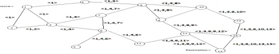
In FANETs, the mobility is very high between the nodes, hence the possibility of route breakage [8] between any two nodes is really high. Hence the packet is lost. Now, to minimize the packet loss, the route is maintained. In the process of data transfer, when the data is transferred from one node to the next an acknowledgement is sent back to the sender node. Now, if the acknowledgement is not received at any level, it means that the link between the nodes has been broken and hence the error message is sent backward from the same route to the source.Fig. 1 given below shows the route discovery procedure of Dynamic Source Routing

(3)

B. Optimized Link State Routing: -

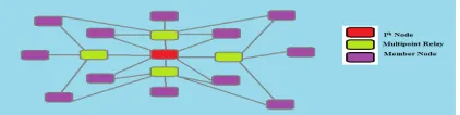
Optimized Link State Routing (OLSR) is table driven pro-active routing protocol in which each node maintains one or more tables containing all the information of all other nodes. All the nodes update their information to maintain the reliable and latest view of information which helps in connection and transfer of information. In OLSR, only the nodes chosen as Multi Point Relays (MPRs) [18], transfer the packets and hence reducing the traffic significantly. Each node selects MPRs which is one hop away from it each of which MPRs maintains the topology information of the network and sends the information from time to time to its neighbour MPRs only and thus reaches the destination node from the source node.

OLSR routing algorithm is divided into 4 parts: -

 Neighbour sensing

 MPR selection

 MPR information declaration

 Routing table Calculation Step 1: Neighbour sensing:

-The neighbour nodes of all the nodes need to be detected with which there exists a bi-directional and direct link. For this each node periodically broadcasts its “HELLO” message to its on hop neighbours. A HELLO message contains:

- A list of addresses of the nodes with which a bi-directional link exists

 A list of addresses of the nodes whose “HELLO” messages are received by this node but have not yet been validated as a bi-directional link If a node finds its own address, a bi-directional link is established.

These “HELLO” messages permits the node to learn the information about its neighbour to two hops. This helps it to select the MPRs. The selected MPRs are described with link status MPR in “HELLO” message. The neighbour table of a node contains the information about its one hop neighbours, the link status (unidirectional, bidirectional or MPRs) to these neighbours and the address till its two hop neighbours.

Step 2: Multipoint Relay Selection: -

Each node of the network selects a set of Multipoint Relays. MPRs are the subset of its one hop neighbours which covers all its two hop neighbours. In order to build the list of two hop nodes from a node, it traces the “HELLO” messages of all its one hop nodes and suffices the nodes with which a bi-directional link exists between the one hop and two hop neighbours. The MPR set need not to be optimal but it should give the benefits of selecting the MPR set. From the next message, the MPR set of that node is declare in the HELLO message. The MPR set is updated when the change in the neighbourhood is detected i.e. either a node is removed from the on hop set or a node is added to it. MPR set is also updated if any change in the link with two hop neighbours is detected.

On the basis of these information, each node builds an MPR selector table in which it includes all the nodes which has selected the node as its MPR along with the MPR sequence number of that neighbour node.

Step 3: MPR information Declaration: -

In order to determine the route to the destination, each node broadcasts specific control messages called as Topology Control (TC) messages which is transmitted as general broadcast messages. These TC messages are transmitted periodically by each node in the network. These messages contain the list of neighbours which has selected the node as Multipoint Relays. The sequence number to these MPR selector set is also attached to it. The information accumulated is used to generate a topology table. The nodes which are not chosen by any other nodes as MPRs so not send any TC messages. The interval between any two TC messages depends upon the change in MPR selector set i.e. if the MPR selector set is changed, the TC message can be sent before the defined interval.

Now, each node maintains a topology table in which it records the information about the topology of the network. Based on this information, a routing table is generated. A particular entry in topology table contains the address of the destination, address of the last hop to that destination, corresponding MPR selector set sequence number.

On receiving TC message the following things happens: -

1. If there exists some entry in the topology table whose last hop address corresponds to the originator address of the TC message and the MPR selector sequence number is greater than the sequence number of the received message then the TC message is discarded, while if the MPR selector sequence number is smaller than the sequence number of the received message then the entry is removed.

(4)

 If there exists some entry in the topology table whose destination address corresponds to the MPR selector address and Last hop node address corresponds to the originator address of that TC message, then the holding time of that entry is refreshed

 Otherwise, a new topological entry is recorded in the table. Step 4: Routing table Calculation: -

Routing table is calculated through following steps:

-1. The new entries are recorded in the table starting with one hop (h=1) neighbour as destination nodes. For each neighbour entry in the neighbour table, whose link status is not uni-directional, a new route entry is recorded in the routing table where next hop address and destination address are both set to neighbour and distance is set to 1. 2. Then the new entries for the destination nodes h+1 hop away are recorded in the routing table. For each topology

entry in topology table, if the destination address does not corresponds to the destinatioin address of any route in the routing table and its last hop address corresponds to destination of a route entry with distance equal to h, then a new node entry is recorded in the routing table where: -

 Destination is set to the destination address in th topology table.

 Next hop is set to next hop of the route entry whose destination is equal to above mentioned last hop address

 Distance is set to h+1. C. Clustering Routing Algorithm: -

We point out that in earlier algorithms it might be possible in Flying Ad-hoc networks that some nodes might be remain uncovered depending on the path and the altitude of the UAVs. Clustering in such environments is feasible and increases the coverage area [21]. In this algorithm, the whole network is divided into clusters of nodes and cluster heads are selected depending on the energy level of nodes in the clusters and the distance from the base station. It is observed that the energy of the nodes gets dissipated at the transmission on each message based on the distance of transmission and no. of bits to be transferred.

There are many studies regarding clustering algorithm is done till now. A basic algorithm is LEACH (Low-Energy Adaptive Clustering Hierarchy) algorithm.

In LEACH algorithm [10], at each clustering round, new CHs are selected by rotating cluster head role among all nodes on the basis of remaining energy levels.Each node sends information about its current location and energy level to the base station in order to obtain load balancing and select CHs with the high energy level.

Step 1: Cluster Formation Algorithm:

Cluster Heads broadcasts an advertisement message (ADV) ADV = node’s ID + distinguishable header.

 Based on the received signal strength of ADV message, each non-Cluster Head node determines its Cluster Head for this round (random selection with obstacle).

 Each non-Cluster Head transmits a join-request message (Join-REQ) back to its chosen Cluster Head using a CSMA MAC protocol [20]. Join-REQ = node’s ID + cluster-head ID + header.

 Cluster Head node sets up a TDMA [11] schedule for data transmission coordination within the cluster.

 TDMA Schedule prevents collision among data messages and energy conservation in non cluster-head nodes. Step 2: The cluster head(s) of m-th cluster formed aggregates the data received from other sensor nodes with its own data and transmits it to the next hop cluster head closer to the base station or to the base station depending on the cluster formation and the shortest distance between the cluster head and the BS. At every transmission or reception made, energy reduction occurs for every node, thereby cluster head rotation was utilized to help prolong the lifetime of the WSN.

D. Data Centric Routing Algorithm: -

Data Aggregation has been put forward as a particularly useful paradigm for wireless routing in sensor networks [12], [13]. The idea is to combine the data coming from different sources enroute eliminating redundancy, minimizing the number of transmissions and thus saving energy. This paradigm shifts the focus from the traditional address-centric

(5)

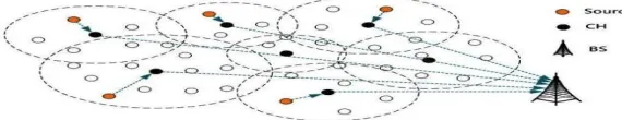
Fig.2 :- Data Centric Routing

The following are three generally suboptimal schemes for generating data aggregation trees: -

 Center at Nearest Source (CNS): In this data aggregation scheme [14], the source which is nearest to the sink acts as the aggregation point. All other sources send their data directly to this source which then sends the aggregated information on to the sink.

 Shortest Paths Tree (SPT): In this data aggregation scheme [14], each source sends its information to the sink along the shortest path between the two. Where these paths overlap for different sources, they are combined to form the aggregation tree.

 Greedy Incremental Tree (GIT): In this scheme [14] the aggregation tree is built sequentially. At the first step the tree consists of only the shortest path between the sink and the nearest source. At each step after that the next source closest to the current tree is connected to the tree.

III.PROPOSED WORK

In this Paper, we are going to suggest an algorithm in which the energy loss per cluster round is decreased and have less number of transmission and a better data hierarchy [19]. The cluster heads on each round is selected from all the multipoint relays of the network on the basis of residual energy of all the multipoint relay (MPRs) nodes and the distance between them and the base station. Now these cluster head chosen act as a base station and further in the cluster of this cluster head, sub-cluster heads are choose from the multipoint relays of the nodes in this cluster on the basis of their distance to this cluster head and energy levels, thus forming a sub cluster which further goes on to make another sub-sub cluster and thus continuing this process till the last node in a particular cluster is covered. Therefore, a hierarchy of clusters is formed.

The whole algorithm is divided into five parts: - Step 1: Neighbour sensing: -

The neighbour nodes of all the nodes need to be detected with which there exists a bi-directional and direct link. For this each node periodically broadcasts its “HEY THERE” message to its on hop neighbours. A “HEY THERE” message contains: -

 A list of addresses of the nodes with which a bi-directional link exists

 A list of addresses of the nodes whose “HEY THERE” messages are received by this node but have not yet been validated as a bi-directional link if a node finds its own address, a bi-directional link is established. These “HEY THERE” messages permits the node to learn the information about its neighbour to two hops. This helps it to select the MPRs. The selected MPRs are described with link status MPR in “HEY THERE” message. The neighbour table of a node contains the information about its one hop neighbours, the link status (unidirectional, bidirectional or MPRs) to these neighbours and the address till its two hop neighbours. Fig. 3 explains the “HEY THERE” message and its usage.

Step 2: Multipoint Relay Selection: -

(6)

set or a node is added to it. MPR set is also updated if any change in the link with two hop neighbours is detected. The nodes which are selected as MPRs by the nodes get an MPR tag attached to it. Fig. 4 shows the selection of MPRs from all the nodes.

Step 3: Cluster Head Selection

All the nodes which have an MPR tag associated to it fight their cause for being cluster heads. The cluster head is selected on the basis of their closeness to base station and their residual energy levels. The energy levels are considered for selecting the cluster heads because at each cluster round, if the same node is chosen the energy of that node decreases significantly. Hence, the node will die out after some cluster round. Hence, for Load Balancing at each round, different cluster heads are selected for transmission of packets to the base station. Fig. 5 shows the selection of cluster head on the basis of distance and the energy remained of a particular node.

Fig. 4:- Representing Multipoint Relays Selection

The dissipated energy of each MPR is calculated on the basis of number of transmissions and the distance between the sender and receiver nodes. This is given by the following equation eq. (1): -

E (K, D, T) =SUMMATION (T) {K * Eelec+ K * Eamp * D2 } eq. (1)

Where K is the number of the bits of packets, Eelecis the energy dissipated in electronic circuits, Eampis the energy

dissipated for transmission in power amplifier and Dis the transmission distance.

On the basis of above given equation the residual energy of each MPR is calculated. After that the Cluster Heads are selected among them by taking into account both the residual energy levels of MPR and the distance between them and the base station using the PBO algorithm [15],[16].

Pseudo code for selection of cluster head and cluster member nodes using proposed pollination based algorithm

Considering BS as the base station, AE is the average energy of the network, CH is the cluster head, and CM is the cluster member, disti and distj are the distance of nodes from the base station. Considering E as the set of energy of all

the nodes, N is the total number of Multipoint Relay nodes.

 All the nodes send their location and present energy to Base Station (BS) .

 BS marks only the higher energy nodes and calculates the AE of the network

 Cluster head Selection (AE, CM, N, CH, E) I <1

While I <= N

If (MPR (i) = True && Ei >AE) then CH (i) = True

Else

CM (i) = True End if

If (MPR (i) = True && MPR (j) = True) For (j = 1; j < N; j++)

If (Ei = Ej) i++ then

Apply the PBO algorithm If (disti<distj) from BS, then CH (i) = True

Else

CH (j) = True End if End if Else

(7)

End while

Step 4: Formation of Cluster Hierarchy: -

The selected clusters are treated as base station and the cluster members are considered to be the fellow nodes in a particular network. Then these nodes find their MPR set by the same method given in the MPR node selection of this section and after finding the MPR, the contest is between them to find the next sub- Cluster Head for that particular network. The next sub cluster head is selected using the same algorithm as discussed “Selection of cluster head” of this section. Now, the further sub clustering of nodes is done by considering the sub-cluster head selected in this round as a base station and further selecting MPRs and cluster heads. This process goes dynamically and recursively till the last node of each cluster is included in the cluster hierarchy.

Fig. 5:- Selection of cluster head.

Step 5: Data Aggregation and transmission: -

All the nodes which wants to transmit the data sends the data to its corresponding sub-cluster heads which aggregates the data received by it with the data that it needs to transmit and the aggregated data is sent further to its sub-cluster head and thus following the same procedure, it reaches the cluster head which aggregates all the data received by it and sends it to the base station which transfers the data to the recipient cluster.

IV.SIMULATION RESULTS

In this paper, simulation analysis is carried out using the net-work simulator NS-2.35[17]. It is a discrete event simulator used in research related to networks. It uses a visual tool called NAM which is Tcl/TK based animation tool for viewing real world packet trace data and network simulation traces. The existing protocols DSR (Dynamic Source Routing), OLSR (Optimized Link State Routing), CAIUAV (Clustering Algorithm in Unmanned Air Vehicles) and our proposed protocol EECA (Energy Efficient Clustering Algorithm) are taken for comparison. The performance parameters are End to End Delay, Packet Delivery Fraction, Number of transmission and energy dissipated. Table 1 shows the parameters used in the simulation and simulation results are shown in Fig 6, Fig 7, Fig 8 and Fig 9.

Table 1:- Simulation Parameters

A. End To End Delay: -

It is the average transmission time taken by data packets to reach from source to destination. If value is large, it means there is congestion in the network and data packets are taking longer to reach the destination than usual. It is observed from the graph (Fig. 6) that EECA has slightly lower end to end delay than other routing protocols though as the number of nodes increases; EECA also has almost similar end to end delay.

Simulation Parameter Value

Network Simulator NS 2.35

Routing Protocols DSR,OLSR,CAIUAV,EECA

No. of Nodes 25,50,75,100,120

Speed of Nodes/ Pause Time 30-40 m/s /15s

Connection Type/ Packet Size CBR/512 bytes

(8)

Fig. 6: - End to End Delay vs Number of Nodes

A. Packet Delivery Fraction: -

It is the fraction of data packets received at destination to packets sent by the source. PDF slightly decreases with increase in number of nodes.From the graph (Fig. 7), we get that the packet delivery ratio is better for EECA, as the packets are transferred in less number of transmissions; hence, the data loss is minimized.

Fig 7: - Packet Delivery Fraction Vs Number of Nodes

B. Energy Consumption:

-Energy consumption is the energy consumed by the network during the simulation. From the graph (Fig. 9), it is clear that the energy consumption by the network during the EECA algorithm has been minimized significantly due to reduced number of transmissions.

Fig. 9: - Energy Consumption Vs Number of Nodes

C. Number Of transmissions:

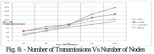
-Transmission is said to have taken place if a packet of data is transmitted from source to destination. Number of Transmissions is the total number of transmissions that has taken place while the duration of the whole simulation. It is clearly observed from the graph (Fig. 8) that the number of transmissions is reduced significantly for EECA algorithm.

Fig. 8: - Number of Transmissions Vs Number of Nodes

V. CONCLUSION AND FUTURE WORK

(9)

the sub cluster heads of the cluster enduring the data. This protocol extends the system’s lifetime as well as optimizes the packet delivery ratio. EECA routing protocol is adapted to a network which is dense and communication is assumed to occur more frequently between large numbers of nodes and EECA routing protocol is much better than the existing routing protocols DSR, OLSR, CAIUAV in terms of end to end delay, packet delivery fraction and number of transmission and energy consumption.

REFERENCES

1. Vanita Rani , Dr. Renu Dhir, “A Study of Ad-Hoc Network” International Journal of Advanced Research in Computer Science and Software Engineering Vol. 3, Issue 3, pp. 135-138, March 2013 .

2. Swati Sharma Dr. Pradeep Mittal, “Wireless Sensor Networks: Architecture, Protocols” International Journal of Advanced Research in Computer Science and Software Engineering, Vol. 3, Issue 1, pp.1-6, January 2013.

3. Surya Mani Sharma, Yugal Verma, Kartik Sekar, “Unmanned Aerial Vehicle (UAV)” International Journal of Science and Modern Engineering (IJISME) Vol. 1, Issue-6,pp. 56-58, May 2013.

4. IlkerBekmezci a, Ozgur Koray Sahingoz a, Samil Temel, “Flying Ad-Hoc Networks (FANETs): A survey” Ad hoc Networks, Vol. 11,Issue 3, pp.1254-1270, 2013.

5. Stefano Rosati, Karol Kru˙zelecki, Gr´egoire Heitz, Dario Floreano, and Bixio Rimoldi, "Dynamic Routing for Flying Ad Hoc Networks”, arXiv:1406.4399v3 [cs.NI], 18 Mar 2015.

6. D.B. Johnson, D.A. Maltz,” Dynamic source routing in ad hoc wireless networks” in: T. Imielinski, H.F. Korth (Eds.), Mobile Computing, The Kluwer International Series in Engineering and Computer Science, vol. 353, pp. 153–181, 1996.

7. Younis, O., Fahmy, S., “HEED: A Hybrid, Energy-Efficient, Distributed Clustering Approach for Ad Hoc Sensor Networks”, Proceedings of IEEE INFOCOM, Mar. 2004. IEEE Transactions on Mobile Computing, Vol. 3, Issue 4, pp. 366-379, October 2004.

8. Neetesh Rajpoot1, Varsha Sharma, Dr. R. C. Jain “Performance Enhancement of DSR Routing Protocol Using Mobile Agents” Certified International Journal of Engineering and Innovative Technology (IJEIT) Vol. 2, Issue 7,pp. 370-374, January 2013.

9. http://www.cs.jhu.edu/~cs647/dsr.pdf DSR.

10. LalitaYadav, Ch. Sunitha “Low Energy Adaptive Clustering Hierarchy in Wireless Sensor Network (LEACH)”, International Journal of Computer Science and Information Technologies (IJCSIT), Vol. 5 (3), pp. 4661-4664, 2014.

11. Kristina Kunert, “TDMA-based MAC Protocols for Wireless Sensor Networks: State of the Art and Important Research Issues”

12. J. Heidemann, F. Silva, C. Intanagonwiwat, R. Govindan, D. Estrin, and D. Ganesan, “Building Efficient Wireless Sensor Networks with Low-Level Naming,” 18th ACM Symposium on OperatingSystems Principles, October 21-24, 2001.

13. W.R. Heinzelman, J. Kulik, and H. Balakrishnan “Adaptive Protocols for Information Dissemination in Wireless Sensor Networks,”

Proceedings of the Fifth Annual ACM/IEEE International Conferenceon Mobile Computing and Networking (MobiCom ’99), Seattle, Washington, August 15-20, 1999.

14. Muhammad Umar Farooq, “Computational Intelligence Based Data Aggregation Technique in Clustered WSN: Prospects and Considerations”, WCECS, Vol. 2, pp.705-1456, 2012.

15. Marwa Sharawi, E. Emary, Imane Aly Saroit, Hesham El-Mahdy ” Flower Pollination Optimization Algorithm for Wireless Sensor Network Lifetime Global Optimization” International Journal of Soft Computing and Engineering (IJSCE), Vol. 4, Issue 3,pp. 54-59, July 2014. 16. K. Balasubramani, K.Marcus, “A Study on Flower Pollination Algorithm and Its Applications,” International Journal of Application or

Innovation in Engineering & Management (IJAIEM), vol.3, 2014. 17. The Network Simulator-2 (NS-2), http://www.isi.edu/nsnam/ns.

18. Dang Quan Nguyen, Pascale Minet, HAL “Analysis of Multipoint Relays Selection in the OLSR Routing Protocol with and without QoS Support”[Research Report], pp.15,2006.

19. Nishi Yadav, PM Khilar,“Hierarchical adaptive distributed fault diagnosis in Mobile ad hoc network using clustering” International Conference on Industrial and Information Systems (ICIIS), IEEE Conference, pp. 7-12, July2010.

20. A. Nasipuri, San Antonio, J. Zhuang, S. R. Das “A multichannel CSMA MAC protocol for multihop wireless networks” Wireless Communications and Networking Conference, vol.3, pp. 1402-1406, 1999.

21. Kavita Tandon, Neelima Mallela, Nishi Yadav“Novel Approach for Fault Detection in Wireless Sensor Network” International Journal of Computer Science and Information Technologies (IJCSIT), Vol. 5 (2) , 2014, 2191-2194

BIOGRAPHY

RISHAB SINHAis B.Tech Student of Computer Science & Engineering, Central University, ITGGV, Bilaspur, and Chhattisgarh, INDIA

VIKASH KUMAR is B.Tech Student of Computer Science & Engineering, Central University, ITGGV, Bilaspur, and Chhattisgarh, INDIA