Fast FSR Variable Selection with Applications to Clinical Trials
Dennis D. Boos, Leonard A. Stefanski
Department of Statistics
North Carolina State University
Raleigh, NC 27695-8203
[email protected], [email protected]
and
Yujun Wu
Sanofi-Aventis
February 11, 2009
Institute of Statistics Mimeo Series # 2609
Summary
A new version of the False Selection Rate variable selection method of Wu, Boos, and Stefanski
(2007) is developed that requires no simulation. This version allows the tuning parameter in
forward selection to be estimated simply by hand calculation from a summary table of output even
for situations where the number of explanatory variables is larger than the sample size. Because
of the computational simplicity, the method can be used in permutation tests and inside bagging
loops for improved prediction. Illustration is provided in clinical trials for linear regression, logistic
regression, and Cox proportional hazards regression.
1
Introduction
Variable selection methods are not used widely in the primary analyses of clinical trials. However,
data collected in these trials are often used for secondary studies where variable selection plays a
role. An example is the PURSUIT cardiovascular study that has generated many papers beyond
the primary paper, Harrington, et al. (1998).
Tsiatis, et al. (2007) proposed model selection in a “principled” approach to covariance
ad-justment that allows variable selection to be used separately and independently in each arm of a
clinical trial. That is primary motivation for our use of variable selection in two other examples,
one repeating their example in linear regression, and a second example using Cox regression.
The method we study is a variant of the False Selection Rate (FSR) method of Wu, Boos, and
Stefanski (2007), henceforth WBS. In that paper, phony explanatory variables are generated, and
the rate at which they enter a variable selection procedure is monitored as a function of a tuning
parameter like α-to-enter of forward selection. This rate function is then used to estimate the appropriate tuning parameter so that the average rate that uninformative variables enter selected
models is controlled to be γ0, usually .05. The variant we develop requires no phony variable
generation, but achieves the same net result. This allows us to estimate the tuning parameter from
a summary table of the Forward Selection variable sequence and associated p-values. We show that if these p-values are monotone increasing, p1 ≤ p2 ≤ . . . ≤ pkT, where kT is the number of predictors, then the implied stopping rule is a version of an adaptive False Discovery Rate (FDR)
method (Benjamini and Hochberg, 1995): choose the model of sizek, where k= max
i:pi≤
γ0(1 +i)
(kT −i)
andpi ≤αmax
,
and αmax is defined later.
The scope of application is large, but we focus on linear, logistic, and Cox regression. Johnson
(2007) illustrates that FSR can be used with other censored data regression techniques such as
Buckley-James (Buckley and James, 1979). Because of the savings in computations, the method
developed here also allows us to consider using the approach in permutation tests, and for improved
prediction via bagging (Breiman, 1996b).
We first review the FSR method in Section 2 and then present the new “Fast” version in Section
Section 5 presents simulation results, and Section 6 illustrates using Fast FSR with bagging to
improve predictions. Section 7 is a short conclusion.
2
The FSR Method in Regression Variable Selection
The variable selection method introduced by WBS is based on adding phony (noise) variables to the
design matrixX and monitoring when they enter a forward selection sequence. The data consists
of an n×1 vector responseY and ann×kT matrix of explanatory variablesX. The variables are
linked by a regression model where each column ofX is associated with a parameterβj. Ifβj 6= 0,
we say thatXj is “informative;” ifβj = 0, we say thatXj is “uninformative.” Our basic quantity
of interest is the FSR given by
γ = E
U(Y,X)
1 +I(Y,X) +U(Y,X)
, (1)
where U(Y,X) and I(Y,X) are the numbers of uninformative and informative variables in the selected model. The expectation is with respect to repeated sampling of the true model (X may
be fixed or random). We include the 1 in the denominator because most models include intercepts
and also because it avoids problems with dividing by 0. Our strategy is to specify a target FSR,
γ =γ0, and to adjust the selection method tuning parameters so thatγ0 is the achieved FSR rate.
Typically,γ0 =.05, although other values might be desired in specific problems.
Now consider a model selection method that depends on a tuning parameterαsuch that model size is monotone increasing in α. For Forward Selection, α is called the significance level for entry or α-to-enter, so that a new variable enters sequentially as long as its p-value to be included in the model (hereafter “p-to-enter”) is ≤ α (and is smaller than all other p-to-enter). For a given data set, let U(α) = U(Y,X) when using the tuning parameter α, that is, U(α) is the number of uninformative variables in the model. Let S(α) denote the total number of variables (excluding the intercept) included in the model.
If we knewU(α), a simple estimator of the FSR in (1) as a function ofαwould be the empirical estimatorU(α)/{1+S(α)}. Then, setting this latter quantity equal toγ0and solving approximately
for α would yield an estimated α as follows, αb = supα{α:U(α)/[1 +S(α)]≤γ0}. This αb is the
largestαsuch that the FSR for the data (Y,X) is not more thanγ0. Thusγ0(αb)≈U(αb)/{1+S(αb)}.
Next, we seek to mimic this approach to get a true estimator that satisfies this approximate equality
BecauseU(α) is unknown, we estimate it with {kT −S(α)}θb(α), where {kT −S(α)} estimates
the total number kU of uninformative variables in the data, and θb(α) is an estimate of the rate
that uninformative variables enter the model using tuning parameter α. We define the target rate function asθ(α) = E{U(α)/kU}.The key idea in WBS for estimatingθ(α) is to generatekP phony
variables, append them to the original set of explanatory variables, and find the number of these
that enter the model when using tuning parameterα, sayUP(α). This process is repeatedB times,
and θb(α) = UP(α)/kP, where UP(α) is the average of UP(α) over the B replications. This is a
bootstrap type step, but note that onlyB sets of phony variables are generated; the original data (Y,X) are used in each replication. Note also that kT −S(α) overestimates the true number of
uninformative variables kU when α is small and underestimates it when α is large. But in the
vicinity of an appropriateα, it is a reasonable estimate. Putting these pieces together yields
b
α= sup
α≤αmax
{α :bγ(α)≤γ0}, where bγ(α) =
{kT −S(α)}θb(α)
1 +S(α) . (2)
Note that bγ(α) = 0 at α = 1 because kT −S(1) = 0 when all the variables are in the model.
Typically, bγ(α) descends to 0 forα in the range [αmax,1] for someαmax because{kT −S(α)}θb(α)
decreases with α for large α. So we do not consider α values beyond αmax = .3, suggested by
extensive simulation results.
WBS studied a number of methods for generating phony variables but recommended permuting
the rows of the originalX leading tokP =kT, the number of phony variables equal to the number
of original variables. A problem with this approach whenkT is large is that one then has to deal
with selecting from 2kT variables each of B times. The computational burden can be heavy, and
some selection procedures may have trouble handling even one run with 2kT predictors.
3
The Fast FSR Method in Forward Selection
3.1 The Forward Selection Method
the sequence of predictors in the order they enter the model the Forward Addition Sequence.
When thep-to-enter are monotone increasing,p1 ≤p2≤. . .≤pkT, Forward Selection(α) chooses a model of sizek, where k= max{i:pi ≤α}. In this case, Forward Selection results in kT nested
models of sizes S(0) = 0, S(p1) = 1, S(p2) = 2, . . .,S(pkT) =kT. We need only consider α values equal to thepi because those are whereS(α) increases.
However, when thep-to-enter are not monotone increasing, we monotonize the original sequence by carrying the largest p forward and use the notationpe1 ≤pe2 ≤. . .≤pekT for these monotonized p-values. Now Forward Selection(α) chooses a model of size k, where k= max{i:pei ≤α}. Note
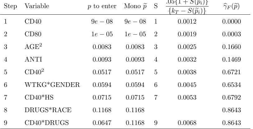
that in this case at least two of these monotonizedp-values must be equal and not all nested models of the Forward Addition Sequence are chosen by Forward Selection(α) as Table 1 illustrates. The “Monope” column has the monotonized p-values, and there are two equal values of 0.1168 at steps 8 and 9 where the originalp-to-enter are not monotone. Thus, model 8 is not possible for Forward Selection(α).
Table 1: Summary from Cox Regression in Group 0 of ACTG 175 Data, kT = 83 Predictors
Step Variable p to enter Mono pe S .05{1 +S(pei)}
{kT −S(pei)} b
γF(pe)
1 CD40 9e−08 9e−08 1 0.0012 0.0000
2 CD80 1e−05 1e−05 2 0.0019 0.0003
3 AGE2 0.0083 0.0083 3 0.0025 0.1660
4 ANTI 0.0093 0.0093 4 0.0032 0.1469
5 CD402 0.0517 0.0517 5 0.0038 0.6721
6 WTKG*GENDER 0.0594 0.0594 6 0.0045 0.6534
7 CD40*HS 0.0715 0.0715 7 0.0053 0.6792
8 DRUGS*RACE 0.1168 0.1168 0.8643
9 CD40*DRUGS 0.0647 0.1168 9 0.0068 0.8643
3.2 Fast FSR
The key quantity in the FSR tuning method is the estimate θb(α) =UP(α)/kP in the numerator of b
γ(α) of (2). The proposed new Fast FSR method simply usesθ(α) =α instead of estimating it by simulation. Then (2) becomes
b
αF = sup α≤αmax
{α:bγF(α)≤γ0} and bγF(α) =
{kT −S(α)}α
1 +S(α) , (3)
where here we define αmax to be the α value where bγF(α) attains its maximum value. These
definitions lead to the simple rule for model size selection,
k(γ0) = max
i:pei ≤
γ0[1 +S(pei)]
kT −S(epi)
andpei ≤αmax
, (4)
where note that the value of αbF is not required. Table 1 illustrates with the results of the Cox
regression discussed later in Example 3. Looking at the bounding column .05{1 +S(pei)}/{kT −
S(pei)}, we see that pe2 = 0.00001 is less than the bound 0.0019, but pevalues after that are not less
than their bounds. Soγ0=.05 leads to a model of size k(.05) = 2.
Oncek(γ0) is found from (4), then the linearity of bγF(α) between jumps gives b
αF =
γ0{1 +k(γ0)}
kT −k(γ0)
.
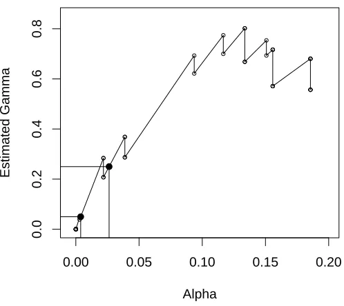
In other words, the estimated α is just the bound in (4) associated with the model size chosen. Figure 1 illustrates: γ0 = .05 chooses αbF = 0.002, and γ0 = .20 chooses αbF = 0.013. Note that
kT = 83 and αmax = 0.12. Although Table 1 does not have the bound for γ0 =.20, we could find
that the chosen model for γ0 =.20 is of size k(.20) = 4 because the last model withbγ(pe) less than
.20 is of size 4. So the last column of Table 1 can be used to choose a model for arbitraryγ0.
3.3 Relationship of Fast FSR to FDR
The False Discovery Rate (FDR) method was introduced into the multiple comparisons literature
by Benjamini and Hochberg (1995) for the case of kT hypothesis tests. FDR is an improvement
over familywise error-rate methods that tend to be fairly conservative. Let the orderedp-values be denoted p(1) ≤ p(2) ≤ · · · ≤ p(kT) and the associated null hypotheses H
0
(1),· · ·, H(k0T). The FDR rule is to rejectH(1)0 ,· · ·H(k)0 , where
k= max
i:p(i)≤ i
kT
γ0
0.00 0.05 0.10 0.15 0.20
0.0
0.2
0.4
0.6
0.8
Alpha
Estimated Gamma
Figure 1: bγF(α) for the Table 1 data. Solid dots are where bγF(α) intersects γ0 = .05 (yielding b
αF = 0.004) and γ0 =.25 (yielding αbF = 0.026). αmax = 0.13. Jumps in bγF(α) occur atpewhere b
γF(pe) are the lower values.
Using our notation, suppose that there are kU true null hypotheses and kI = kT −kU false
hypotheses, and let U be the number of true null hypotheses that are rejected out of a total of S hypotheses that are rejected using (5). If the test statistics are independent, then Benjamini and
Hochberg (1995) proved that FDR= E{U/S |S >0}P(S >0)≤γ0kU/kT. That is, (5) controls the
FDR to be less than or equal toγ0becausekU/kT ≤1.Benjamini and Yekutieli (2001) extended the
method to certain types of dependencies in the test statistics and noted that the bound applies to
any type of dependency ifγ0 in (5) is replaced byγ0/Pki=1T i−1
. Benjamini and Hochberg (2000)
and Benjamini, Krieger, and Yekutieli (2006) give adaptive versions of (5) whereby an estimatebkU
ofkU is used, replacingγ0 byγ0kT/bkU andγ0kT/{bkU(1 +γ0)}, respectively. Thus, the first of these
adaptive procedures uses the bound
p(i) ≤ i
kT
γ0
kT b
kU
= iγ0
b
kU
, (6)
whereas the Fast FSR procedure uses
e
pi ≤
{1 +S(epi)}γ0
kT −S(pei)
. (7)
Clearly, then, the Fast FSR procedure is a type of adaptive FDR applied to the monotonized
in the numerator of (7) arises from the definition of FSR with 1 +S in the denominator instead of S, ii) the use of kT −S(epi) in place of a fixed estimate bkU for the number of uninformatives. We
originally considered using a fixed estimate and then iterating but found that it typically led to the
same chosen model as (7).
The only use of FDR in regression that we are aware of is due to Bunea, Wegkamp, and
Au-guste (2006). They proposed using the conservative bound iγ0/kT Pki=1T i−1
with full model
p-values and show that under certain regularity conditions, the method results in consistent vari-able selection. However, we tried this approach using the less conservative boundiγ0/kT with our
simulations, and found it not competitive unless the predictors are uncorrelated.
3.4 Justification of θ(α) = α
First consider Fast FSR in the case of normal linear regression, known error varianceσ2, and
orthog-onal design matrixX. If thejth variable is uninformative, then itsp-value is uniformly distributed on (0,1). Also, all the p-values are independent. Thus the number of uninformative variables in-cluded in the model when using forward selection with tuning parameter α is binomial(kU, α). In
this case, all conditions for using FDR are met, and we could appeal to FDR theorems to justify the
Fast FSR procedure because of the similarity of Fast FSR to adaptive FDR. In general, though, the
forward selection p-values to enter do not have the properties required for formal FDR theorems. For the orthogonal case, estimatingσ2 in the usual way at each step of forward selection alters the uniform distribution and independence slightly, but the expected number of uninformative variables
in the model should still be close tokUα.
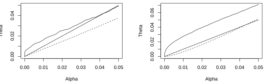
Simulations for the case ofX generated from independent normal variables show that θ(α) is very close to α, but that bγF from (3) is larger than the true γ(α) = E[U(α)/{1 +S(α)}] because
kT −S(α) is not a perfect estimator of kU. To illustrate a situation that is far away from the
orthogonal X case, the left panel of Figure 2 plots an “oracle” estimate of θ(α) (solid irregular line) given by the average of U(α)/kU from 1000 Monte Carlo replications of a model where the
matrices X were generated with autocorrelated N(0,1) variables (ρ=.7). The situation is similar to Model H3 in WBS:n= 150,kT = 21 total variables,kI= 10 variables with nonzero coefficients
at variables 5-9 and 12-16 with values (25,16,9,4,1), respectively, and then multiplied by a constant
0.00 0.01 0.02 0.03 0.04 0.05
0.00
0.02
0.04
Alpha
Theta
0.00 0.01 0.02 0.03 0.04 0.05
0.00
0.02
0.04
0.06
Alpha
Theta
Figure 2: θ(α) curves. Left panel: The Fast FSR proposal θ(α) = α (solid straight line) and averages of U(α)/kU (solid line, s.e.’s ≤ .002) that approximate θ(α) and averages of θb(dashed
line, s.e.’s ≤ .0002) from 1000 Monte Carlo replications of the H3 model: n = 150, R2 = .35,
kT = 21, kI = 10, kU = 11. X matrices were generated from a AR(1) standard normal process
with ρ = .7. The right panel is from 1000 replications of the M20 model: n = 200, R2 = .50,
kT = 80, kI = 20, kU = 60. X matrices were generated from a AR(1) standard normal process
withρ=.6.
Fast FSR. The dashed line is the average of θbfrom using the phony variable method of WBS. The reason the latter is less noisy than the solid oracle line is because each θbis based on 500 bootstrap averages. We have plotted for α∈(0, .05), but the estimated α chosen by the FSR method in this situation with γ0 = .05 is ≈ .01. Thus, most of the “action” occurs on the extreme left side of
both plots. On that portion of the left graph, the average of θb(α) from regular FSR with phony variables is quite close to θ(α) =α of Fast FSR.
As a second illustration, we consider a case with n = 200, kT = 80, kI = 20 nonzero βs all
equal, R2 =.5, and theX matrices generated from an AR(1) process with ρ=.6. In addition, we
randomly permute the columns of X for each Monte Carlo data set. The right panel of Figure 2
gives plots analogous to the left panel of Figure 2. Here we see that the regular phony-generated
FSR method and Fast FSR are very close to one another, justifying the replacement of regular FSR
and poor prediction. The poorer correspondence betweenθ(α) and θ(α) =α in the right panel is due to high correlation between the informative and noninformative variables.
4
Examples
Example 1. Logistic Regression in the PURSUIT Study. The Platelet Glycoprotein IIb/IIIa in
Unstable Angina: ReceptorSuppressionUsingIntegrilinTherapy (PURSUIT) study was a
multi-country, multi-center, double-blind, randomized, placebo-controlled study comparing a regimen of
integrilin or placebo added to aspirin and heparin in 10,948 patients (Harrington, et al., 1998).
We consider a subset of patients from North America and Western Europe. The primary endpoint
of death or heart attack in the first 30 days was significantly reduced in patients randomized
to integrilin therapy, but further analysis revealed that the effect was strongest in males and in
patients treated with percutaneous coronary intervention (PCI). We investigate whether other
baseline characteristics are associated with the primary endpoint.
We used forward selection in logistic regression after forcing in five variables: treatment, gender,
and PCI indicators, and interactions of the treatment indicator with the gender and PCI indicators.
In a first run of Forward Selection on 34 variables and their interactions with gender (kT = 68
variables not counting the included variables), we selected the top 14 main effects using a generous
α = .15 in the forward selection. To these 14 we added their interactions with gender and the squares after centering of the five continuous main effects in the top 14. Thus, in the second run we
selected on 14+14+5=33 variables. However, we use kT = 68 + 12 = 80 in the Fast FSR analysis
because that would be the number of variables used for selection if we had added all 12 continuous
quadratic terms. The main reason to do variable selection in two stages is that the sample size of
4888 complete cases increases to 5360 when we drop 20 of the original variables.
Fast FSR chose 12 additional terms of potential interest, including two quadratic terms and
one interaction with gender. For the interactions and quadratic terms, we enforced the hierarchy
principle that interactions can enter only after the associated main effects have entered, but only
minor differences are introduced by not enforcing it. Having chosen S = 12 terms, the estimated α-to-enter is just the associated bound,αbF =.0096.
mean responses in the different treatment groups using model selection methods. For two treatment
groups, labeled 0 and 1, the adjusted estimate of the mean difference is given by
n1
nY
(1)
+n0 nYb
(1)
0 −
nn0
n Y
(0)
+n1 nYb
(0) 1
o
, (8)
wheren0 andn1 are the sample sizes in groups 0 and 1,n=n0+n1,Y (1)
and Y(0) are the sample means. Furthermore, Yb0(1) is the predicted Treatment 1 mean based on the explanatory variables from Group 0 using a model developed from the Group 1 data, andYb1(0) is similarly the predicted Treatment 0 mean from the Group 1 data. Thus, the estimate is an intuitive difference of weighted
means. Each weighted mean is essentially an estimate of the appropriate estimate if each group
could receive both treatments. In their approach, Tsiatis, et al. (2007) suggest that the modeling
in each group be done separately, ideally by independent statisticians, each using a model selection
method of their choosing. An alternative approach is to have a very carefully specified protocol
for doing the model selection in each group, thus avoiding the possibility of biasing the estimated
treatment mean difference by choice of models.
We should mention that this separate-group covariance analysis is somewhat different from the
common approach of testing for significance of an indicator variable for treatment in the presence
of a number of covariates modeled within the full combined data. The idea is that with separate
modeling there is much less chance to “explore” the data to find the covariance model producing
the most significant treatment effect.
We use the example from Tsiatis, et al. (2007) to illustrate Fast FSR in this context. The data
are from AIDS Clinical Trials Group Protocol 175 (ACTG 175, Hammer, et al., 1996) withn0= 532
in the zidovudine monotherapy group (Group 0), and three other treatments groups combined to
yieldn1= 1607 subjects in Group 1. Following Tsiatis, et al. (2007), we look for a mean difference
in CD4 counts at approximately week 20 (±5 weeks) using 12 possible baseline covariates: CD4
counts (CD40), CD8 counts (CD80), age in years (AGE), weight in kilograms (WTKG), Karnofsky
scores (KARN, 0-100), hemophilia indicator (HEMO, 1=yes), homosexual indicator (HS, 1=yes),
history of intravenous drug use indicator (DRUGS, 1=yes), race (RACE, 0=white, 1=non-white),
gender (GENDER, 1=male), history of antiretroviral use (ANTI, 0=naive, 1=experienced), and
symptomatic status (SYMP, 1=present). The first 5 are continuous and the rest are binary. Tsiatis,
et al. (2007) used forward selection with fixed entrance levelα =.05 along with the 12 explanatory variables (Forward-1 in their notation) and then with the full quadratic model (Forward-2) having
4 and 7 variables selected, respectively, for groups 0 and 1, and Forward-2 had 4 and 10 variables
selected.
For the 12-variable linear case, Fast FSR chose 3 variables in Group 0 (αb=.022) and 7 in Group 1 (αb =.080). For the quadratic model we centered the 5 continuous variables in both groups by subtracting overall means before creating squared and interaction terms. For the 83 variables of the
full quadratic case, Fast FSR chose 4 variables in Group 0 (αb=.003) and 8 in Group 1 (αb=.006). The estimates from (8) and associated tests were all similar for these different modeling approaches
with highly significant approximately normal test statistics ≈10.
For a more inferentially challenging example, we randomly sampledn′
0= 100 from the 532 Group
0 cases andn′
1= 100 from the 1607 Group 1 cases. Then we repeated this sampling forn′′0 = 200 and
n′′
1 = 200. Because there might be concern that the standard errors given in Tsiatis, et al. (2007)
for (8) (see their equations 18 and 19) could be affected by model selection, we used approximate
permutationp-values based on 100,000 random permutations. Each permutation employed all data manipulations such as centering and model selection within each group used to calculate the test
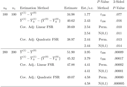
statistic. Table 2 gives the results. The normal approximations are quite good even for sample
sizes of 100: the two-sided permutationp-values are .010 and .013 for linear and quadratic covariate adjustments, respectively, compared to .011 and .014 for the normal approximations.
Fast FSR facilitated computation of the permutation p-values in reasonable time. Fast FSR, however, did not select many variables; 2 and 1 for the linear case (kT = 12), 1 and 1 for the
quadratic case (kT = 83) for n′0 = n′1 = 100; and 3 and 1 (linear), and 3 and 1 (quadratic) for
n′′
0 = n′′1 = 200. Therefore, because little selection actually occurred, it is not surprising that
the standard error and normal approximation work well here. There is also a hint of a practical
suggestion here: for small samples, it may be wise to just select from the linear terms, leaving
quadratic models for larger sample sizes.
Example 3. Variable Selection in Cox Regression. Lu and Tsiatis (2007) used the ACTG 175 data from the previous example to illustrate covariate adjustment with a composite survival
endpoint defined as the first time a subject’s CD4 count decreased to 50% of baseline or they
developed an AIDS-defining event or they died. In the original paper, Hammer et al. (1996), this
endpoint was used to show the value of combined therapies compared to the use of zidovudine
Table 2: Summary of Results for ACTG 175 Subsample Data
P-Value 2-Sided n0 n1 Estimation Method Estimate Est./s.e. Method P-Value
100 100 Y(1)−Y(0) 34.98 1.77 t198 .077
Y(1)−Y(1)0 − {Y(0)−Y(0)0 } 40.62 2.43 t198 .016
Cov. Adj: Linear FSR 39.69 2.54 Perm. .010
2.54 N(0,1) .011
Cov. Adj: Quadratic FSR 38.97 2.44 Perm. .013
2.44 N(0,1) .014
200 200 Y(1)−Y(0) 51.90 3.95 t398 .00009
Y(1)−Y(1)0 − {Y(0)−Y(0)0 } 45.32 3.79 t398 .00017
Cov. Adj.: Linear FSR 47.88 4.41 Perm. .00002
4.41 N(0,1) .00001
Cov. Adj.: Quadratic FSR 49.07 4.58 Perm. .00000
4.58 N(0,1) .000005
Perm. p-values based on 100,000 random permutations, standard error ≤.0003.
(kT = 83) of variables to select a proportional hazards model. PROC PHREG in SAS was used
to get the forward sequence of variables and p-values based on score statistics displayed in Table 1, used previously in Section 3.2 to illustrate Fast FSR. As mentioned previously, for γ0 = .05,
we choose a two variable model, with terms CD40 and CD80. The associated estimated α is
b
αF =.05(1 + 2)/(83−2) =.00185.
5
Simulation Results
Here we report on three sets of simulations, two for linear regression and one for logistic regression.
5.1 Linear Regression with Fixed X
Two 150×21 design matrices were generated from N(0,1) distributions, independent in the first
case (ρ = 0) and autocorrelated, AR(1) with ρ = 0.7, in the second case. In addition, we added squares of the 21 original variables to make akT = 42 case and then added all pairwise interactions
to make a full quadratic case withkT = 252. In all cases, the added variables have true coefficients
equal to 0. We ran simulations for kT = 21, kT = 42, kT = 100, andkT = 252, but report below
only on the kT = 42 andkT = 252 (not displayed) because results for the other two cases can be
anticipated from the ones reported.
The five mean models considered are the same as in WBS: H0=all β=0; H1=2 equal nonzero βs for variables 7 and 14; H2=6 nonzero βs at variables 6-8 and 13-15 with values (9,4,1); H3=10 nonzero βs at variables 5-9 and 12-16 with values (25,16,9,4,1), respectively; and H4=14 nonzero βs at variables 4-10 and 11-17 with values (49,36,25,16,9,4,1), respectively. These nonzero βs were multiplied by a constant to make the theoretical R2 =.35, where theoretical R2 =µTµ/{µTµ+
nσ2},µ=Xβ, and σ2 is the error variance.
For simplicity we do not enforce the hierarchy (requiring linear terms to come in the model before
related quadratic terms). In fact, here the addition of the quadratic and interaction variables is
just a simple way to increase the number of explanatory variables.
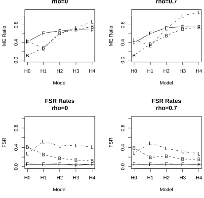
Figure 3 gives average Model Errors and FSR rates for the Fast FSR and minimum BIC methods
based on the Forward Addition Sequence, and for the LASSO (Tibshirani, 1996) using 5-fold
cross-validation averaged 10 times. The Model Error for one data set is n−1Pn i=1
n b
f(xi)−µi o2
,where
b
f(xi) is the prediction for the ith case and µi is the true mean for that case. The FSR for one
data set isU(Y,X)/{1 +I(Y,X) +U(Y,X)},whereI(Y,X) and U(Y,X) are the numbers of informative and uninformative variables in the selected model. These measures are averaged over
the 100 generated data sets. The Fast FSR and minimum BIC methods use the leapspackage in
R, and the LASSO was computed with thelarspackage in R. Figure 3 displays Model Error ratios
obtained by dividing the minimum Model Error of all models in the Forward Addition Sequence
by the method Model Error. Thus large values indicate good performance. The minimum BIC
method is based on choosing the model from the Forward Addition Sequence that has the lowest
BIC value.
F
F F F F
0.0
0.4
0.8
Model
ME Ratio
H0 H1 H2 H3 H4
B B B B B L L L L L
ME(min)/ME
rho=0
F FF F F
0.0
0.4
0.8
Model
ME Ratio
H0 H1 H2 H3 H4
B B B B B L L L L L
ME(min)/ME
rho=0.7
F F F F F
0.0
0.4
0.8
Model
FSR
H0 H1 H2 H3 H4
B B
B B B
L L
L L L
FSR Rates
rho=0
F F F F F
0.0
0.4
0.8
Model
FSR
H0 H1 H2 H3 H4
B
B B B B
L L L L L
FSR Rates
rho=0.7
Figure 3: Model Errors divided into the minimum Model Error possible for forward selection and
FSR rates for Fast FSR (F), BIC (B), and LASSO (L). Based on 100 Monte Carlo replications for
a situation with n= 150, R2 =.35, and kT = 42. Standard errors for the Model Error ratios are
bounded by .06 except for Model H0 and range from .01 to .04 for the FSR rates.
models with kT = 252 (not displayed). In fact we had to limit the models searched to the first 60
of the Forward Addition Sequence to even get these BIC results. The BIC curve keeps decreasing
when kT is too large. The LASSO does well in terms of Model Error and even beats the best
possible Model Error of the Forward Addition Sequence in H4 for kT = 42.
Basically, the LASSO is better than Fast FSR for all the H4 cases and one of the H3 cases.
However, the LASSO has much higher FSR rates because it admits many variables. In thekT = 252
true model for H4 has 14 nonzero coefficients. The minimum Model Error “oracle” method had
average model sizes of 5.1 and 2.9 for H4 at kT = 252. So Fast FSR has low model size apparently
to achieve the FSR rate near .05, but in that H4 case it is not too far from the correct average
optimal size.
In general, these simulations suggest that Fast FSR has reasonable Model Error and close to
the advertised .05 FSR rate. BIC fails miserably forkT = 252. The LASSO has good Model Error
for larger models, but at the cost of a high FSR.
5.2 Logistic Regression with Fixed X
For logistic regression, we ran simulations similar to the previous section, but the data generation
process is a little more complicated. First, data were generated from a linear model with logistic
errors using the βs of the previous section adjusted so that theoretical R2 =.35. Then, binary Y
were created by letting Y = 1 if the original linear model Y was greater than than β∗
0, and Y = 0
otherwise. The values of β∗
0 were set so that the unconditional probability P(Y = 1) was 0.1 or
0.5. Details may be found in Wu (2004).
F
F
F F F
0.0
0.4
0.8
Model
ME Ratio
H0 H1 H2 H3 H4
B
B
B B B
P
P
P P P
F
F F
F
F
0.0
0.4
0.8
Model
ME Ratio
H0 H1 H2 H3 H4
B
B
B B
B
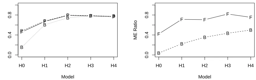
Figure 4: Logistic regression average Model Errors divided into the minimum Model Error possible
for forward selection using Fast FSR (F), BIC (B), and FSR with phony variable generation (P).
Based on 100 Monte Carlo replications for a situation with n = 150, R2 = .35, ρ = 0.7, P(Y = 1) = 0.5, andkT = 21 (left panel) andkT = 100 (right panel). Standard errors for the Model Error
In Figure 4 are Model Errors for thekT = 21 andkT = 100 situations withP(Y = 1) =.5 and
ρ = 0.7. In the left panel of Figure 4, we have plotted both Fast FSR (F) and the original phony generated FSR (P), but they are nearly identical. In the left panel, the minimum BIC method is
almost the same as the FSR methods except in the null model with no informative variables. For the
right panel withkT = 100 (21 linear terms, 21 squared terms, and 58 interaction terms), minimum
BIC degrades dramatically. For this case, we even limited the search to the first 20 members of the
Forward Addition Sequence. As in the previous section, the FSR methods have FSR rates close
to .05 although some are closer to .10 (not displayed), and the BIC FSR rates are much higher.
The original phony variable FSR method was not run for the kT = 100 case because of computer
time. Our simulations suggest that Fast FSR can be used effectively in logistic regression, at least
in these relative sparse models. SAS Proc Logistic was used for obtaining the Forward Addition
Sequences.
5.3 Linear Regression with Random X
The previous sections used models that were relatively sparse, especially when adding uninformative
interaction terms. Thus, we wanted to provide a more challenging situation for forward selection
and our Fast FSR method.
The data were generated from a mean zero normal AR(1) process, this time with ρ =.6 and kT = 80 variables. However, we transformed 20 of the variables by taking their absolute value and
dichotomized another 20 variables asI(Xij >0). Finally, the 80 variables were randomly permuted
and rescaled to have sample mean equal to 0 and sample variance equal to 1 before creating the
responses. This process was repeated for each of the 100 design matricesX in the simulation. Thus,
this is a case with random design matrices, in contrast to the two previous simulation settings. The
models used were M0=no informative variables, M5=5 equal nonzero βs, M10=10 equal nonzero βs, M20=20 equal nonzeroβs, and M40=40 equal nonzeroβs. Theβs were multiplied by a constant in each case to have theoretical R2= 0.5.
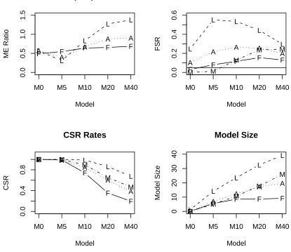
The top left panel of Figure 5 gives Model Error ratios defined in Section 5.1. We see that similar
to previous results, Fast FSR performs well for sparse models with few informative predictors, but
not as well for the larger models. Here, that tendency is accentuated because there are even larger
F F F F F 0.0 0.5 1.0 1.5 Model ME Ratio
M0 M5 M10 M20 M40
L L L L L A A A A A
ME(min)/ME
F FF F F
0.0 0.2 0.4 0.6 Model FSR
M0 M5 M10 M20 M40
L
L L
L
L
A
A A A A
M M M M M
FSR Rates
F F F F F 0.0 0.4 0.8 Model CSRM0 M5 M10 M20 M40
L L L
L L A A A A A M M M M M
CSR Rates
FF F F F
0 10 20 30 40 Model Model Size
M0 M5 M10 M20 M40
L L L L L A A A A A M M M M M
Model Size
Figure 5: Model Errors divided into the minimum Model Error possible for forward selection, FSR
rates, CSR rates, and Model Sizes for Fast FSR (F), LASSO (L), LSA (A), and minimum Model
error (M). Based on 100 Monte Carlo replications for a situation with n= 200, R2 =.5, ρ = .6, andkT = 80. Standard errors for Model Error ratios are≤.03 except for Model M0; for FSR rates
are≤.04; for CSR rates are≤.02; for Model Size are ≤.89.
Selection in this type situation—note that the LASSO is much better at M20 and M40 than the
oracle minimum Model Error for the Forward Addition Sequence. We also added another method,
the Least Squares Approximation (LSA) for LASSO estimation of Wang and Leng (2007) using a
BIC stopping rule (see their equation 3.5). Marked with an “A” in Figure 5, the LSA performs
intermediate to the LASSO and Fast FSR, perhaps not a surprising result since its BIC stopping
rule tends to choose smaller models than regular LASSO. We also give average FSR rates, CSR rates
(proportion of informative predictors selected), and model size. CSR is complementary to FSR—
together along with average model size they give a fuller picture of a model selection procedure’s
characteristics. Here the LASSO chooses large models sizes and therefore has high FSR rates and
CSR rates. The LSA is in between those two.
The FSR rate of Fast FSR exceeds the target .05 rate in Models M10-M40 (c.f., Figure 3). The
problem lies in the higher correlation between informative predictors and noninformative predictors
and the larger models. Although we have not displayed the phony variable version of FSR, it
performs similarly to Fast FSR. We repeated some simulations for the situation of Figure 3 using
randomly permuted X matrices, and we see elevated FSR rates. Also, we repeated simulations
like those in Figure 5 but without the random permuting of columns, and the FSR rates were as
advertised (near .05). In all cases, the informative variables are in the first columns so that without
permuting columns, the informative variables are not very correlated with the uninformative ones.
Thus we believe the problem is with the increased correlation between informative predictors and
noninformative predictors induced by permuting the columns. Both Fast FSR and regular
phony-generated FSR are based on independence between these two sets of predictors.
We could develop an improved FSR method to handle this correlation problem, but it is not
clear that we want to. In Figure 5 we have also given results for the oracle minimum Model Error
method, marked “M” on the graph. Note that its FSR rates and Model Sizes are considerably
higher than Fast FSR. Thus, to achieve FSR rates around .05 as advertised, the Model Error and
CSR performance of such an improved FSR method would be much worse. So, the quandary is
that for large models with high correlation among the explanatory variables, any model selection
procedure based on Forward Selection cannot have both low FSR rates and good Model Error. In
the next section, we show that bagging Fast FSR can recover good Model Error performance in
these situations.
6
Bagging
Breiman (1996a, 1996b) showed that some model selection procedures are unstable in the sense
that perturbing the data can result in selection of very different models. One of his proposals for
improving model selection stability is bagging, essentially averaging selected models over bootstrap
data sets. The simplicity of Fast FSR enables its use in bagging as follows: Randomly draw with
replacement from the pairs (Yi,xi),i= 1, . . . , n; run Fast FSR on the bootstrap sample and obtain b
Note that with this model averagingβ∗ typically has no zeroes even though each βb∗ has many
zeroes—so there is no variable selection in the averaged model. In our simulations, bagging Fast
FSR had a large improvement over Fast FSR in terms of Model Error for the less-sparse sampling
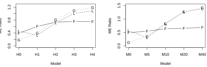
situations. The left panel of Figure 6 repeats simulations from the right panel of Figure 3, and the
right panel repeats the upper left panel of Figure 5 . In the left panel of Figure 6, bagging Fast FSR
is better in terms of Model Error than Fast FSR for models H2-H4 and better than the LASSO in
Models H1-H4. Similar results are found in the right panel of Figure 6 except that bagging Fast
FSR and the LASSO are nearly identical for models M5-M40. Bagging Fast FSR is better than the
oracle minimum Model Error for the Forward Addition Sequence in 4 of the 10 models displayed
in Figure 6 (where the Model Error ratios are>1).
F
F
F F F
0.0
0.4
0.8
1.2
Model
ME Ratio
H0 H1 H2 H3 H4
G
G
G
G G
L
L
L
L L
F F
F F F
0.0
0.5
1.0
1.5
Model
ME Ratio
M0 M5 M10 M20 M40
L
L
L
L L
G
G
G
G
G
Figure 6: Model Errors divided into the minimum Model Error possible for forward selection, Fast
FSR (F), LASSO (L), and Bagged Fast FSR (G). Based on 100 Monte Carlo replications for the
situation in the right side of Figure 3 withn= 150, R2 =.35,ρ=.7, andkT = 42 (left panel) and
for the situation of Figure 5 with n= 200, R2 =.5, ρ =.6, and kT = 80 (right panel). Standard
errors for the Model Error ratios are bounded by .03 except for Model M0.
A feature of the bagged Fast FSR method is that the αb chosen by Fast FSR on the bootstrap datasets is larger on average than those chosen by Fast FSR on the parent data sets. Our
expla-nation for this phenomenon is that in the bootstrap world created by randomly resampling pairs,
the “true” model is effectively the full least squares solution, and thus there are no non-zeroβs in that world. Thus, it makes sense for Fast FSR to try and pick larger models on the bootstrap data
compared to small underfitting.
Clearly, bagging seems to be useful for prediction (as measured by Model Error) in the larger
models used in Figure 6. Can we anticipate when it will be useful to use bagging of Fast FSR
instead of merely Fast FSR? Yuan and Yang (JASA, 2005) suggested a measure of instability given
by the derivative of I(c) atc= 0 where
I(c) = 1 Mσb
M X
j=1 "
1 n
n X
i=1 n
b
fj(xi)−fb(xi) o2#1/2
,
b
f(xi) is the prediction from a selected model, bσ is an estimate of the error standard deviation
from the selected model, and fbj(xi) is the prediction from the selected model from the jth ofM
bootstrap data sets of the form (Ye1,x1), . . . ,(Yen,xn), whereYei =Yi+Wi and W1, . . . , Wn are iid
from aN(0, c2σb2) distribution. The derivative atc= 0 ofI(c) is called the “Perturbation Instability
in Estimation” (PIE) and is estimated by regression through the origin using a grid ofcvalues and the correspondingI(c) values. In our implementation, we used M = 100 andc= (.1, .3, .5.,7, .9). Yuan and Yang (2005) recommend that some type of model averaging approach be used when the
PIE values are higher than .4 to .5.
For the simulation data sets used to make the right panel of Figure 6, the average values of
PIE with standard deviations in parentheses were PIE(M0) = .09 (.06), PIE(M5) = .35 (.10),
PIE(M10) = .66 (.09), PIE(M20) = .78 (.11), PIE(M40) = .84 (.10). Thus, from these averages
and standard deviations, the Yuan and Yang (2005) rule of thumb suggests bagging most of the
time when sampling from models M10, M20, and M40, precisely the models in Figure 6 where
bagging improves over Fast FSR in terms of Model Error. So the good news is that situations
where bagging is needed to obtain good predictions can be identified.
7
Conclusion
Fast FSR in Forward Selection provides an intuitive choice of model size (and associated αbF) that
is a type of adaptive FDR applied to the monotonized forward selection p-values. It can be used with essentially any regression method; we have used it with linear, logistic, and Cox regression.
Forward selection’s prediction performance can degrade when there are a large number of highly
correlated predictors with a large number of informative predictors relative to sample size. Although
suggest bagging Fast FSR for predictions. Computing the PIE measure aids in making the choice
between regular Fast FSR and bagged Fast FSR.
ACKNOWLEDGMENTS
We thank Duke Clinical Research Institute for the PURSUIT data and Marie Davidian and Butch
Tsiatis for providing the ACTG 175 data and preprints of papers. FSR programs in SAS and R are
available at http://www4.stat.ncsu.edu/~boos/var.select. This work was supported by NSF
grant DMS-0504283.
REFERENCES
Benjamini, Y., and Hochberg, Y. (1995). Controlling the false discovery rate: a practical and
powerful approach to multiple testing. Journal of the Royal Statistical Society B,57, 289-300.
Benjamini, Y., and Hochberg, Y. (2000). On the adaptive control of the the false discovery rate in
multiple testing with independent statistics. Journal of Educational and Behavioral Statistics
25, 60-83.
Benjamini, Y., and Yekutieli, D. (2001). The control of the the false discovery rate in multiple
testing under dependency. Annals of Statistics 291165-1188.
Benjamini, Y., Krieger, A. M., and Yekutieli, D. (2006). Adaptive linear step-up procedures that
control the false discovery rate. Biometrika 93491-507.
Breiman, L. (1996a). Heuristics of instability and stabilization in model selection. The Annals of Statistics24, 2350-2383.
Breiman, L. (1996b). Bagging predictors. Machine Learning 24, 123-140.
Buckley, J., and James, I. (1979). Linear regression with censored data. Biometrika 66, 429-436.
Bunea, F., Wegkamp, M. H., and Auguste, A. (2006).Consistent variable selection in high
Hammer, S. M., Katzenstein, D. A., Hughes, M. D., Gundaker, H., Schooley, R. T., Haubrich, R.
H., Henry, W. K., Lederman, M. M., Phair, J. P., Niu, M., Hirsch, M. S., and Merigan, T. C.,
for the Aids Clinical Trials Group Study 175 Study Team (1996). A trial comparing nucleoside
monotherapy with combination therapy in HIV-infected adults with CD4 counts from 200 to
500 per cubic millimeter. The New England Journal of Medicine333, 1081-1089.
Harrington, R. A. for the PURSUIT Trial Investigators (1998). Inhibition of platelet glycoprotein
with eptifibatide in patients with acute coronary syndromes. The New England Journal of Medicine339, 436-443.
Hastie, T., Tibshirani, R. J., Friedman, J. (1996). The elements of statistical learning. New York: Springer.
Johnson, B. A. (2007). Variable selection in semiparametric linear regression with censored data.
To appear inJournal of the Royal Statistic Society, Series B.
Lu, X., and Tsiatis, A. A. (2007). Improving the efficiency of the log-rank test using auxiliary
covariates. To appear inBiometrika.
Miller, A. (2002). Subset selection in regression. CRC Press (Chapman & Hall).
Tibshirani, R. J. (1996). Regression shrinkage and selection via the LASSO. Journal of the Royal Statistic Society, Series B 58, 267-288.
Tsiatis, A. A., Davidian, M., Zhang, M., and Lu, X. (2007). Covariate adjustment for two-sample
treatment comparisons in randomized clinical trials: A principled yet flexible approach. To
appear inStatistics in Medicine.
Wang, H., and Leng, C. (2007). Unified LASSO estimation via least squares approximation. To
appear inJournal of the American Statistical Association.
Wu, Y. (2004). Controlling variable selection by the addition of pseudovariables. Unpublished
doctoral thesis, North Carolina State University, Statistics Dept.
Wu, Y., Boos, D. D., Stefanski, L. A. (2007). Controlling variable selection by the addition of
pseudovariables. Journal of the American Statistical Association102, 235-243.