Fault Detection in Differential Algebraic Equations.

(1)

ABSTRACT

SCOTT, JASON RODERICK. Fault Detection in Differential Algebraic Equations. (Under the direction of Stephen L. Campbell.)

Fault detection and identification (FDI) is important in almost all real systems. Fault detec-tion is the supervision of technical processes aimed at detecting undesired or unpermitted states

(faults) and taking appropriate actions to avoid dangerous situations, or to ensure efficiency in

a system. This dissertation develops and extends fault detection techniques for systems modeled by differential algebraic equations (DAEs).

First, a passive, observer-based approach is developed and linear filters are constructed to

identify faults by filtering residual information. The method presented here uses the least squares completion to compute an ordinary differential equation (ODE) that contains the solution of

the DAE and applies the observer directly to this ODE. While observers have been applied to

ODE models for the purpose of fault detection in the past, the use of observers on completions of DAEs is a new idea. Moreover, the resulting residuals are modified requiring additional

analysis. Robustness with respect to disturbances is also addressed by a novel frequency filtering

technique.

Active detection, as opposed to passive detection where outputs are passively monitored,

allows the injection of an auxiliary control signal to test the system. These algorithms compute

an auxiliary input signal guaranteeing fault detection, assuming bounded noise. In the second part of this dissertation, a novel active detection approach for DAE models is developed by

tak-ing linear transformations of the DAEs and solvtak-ing a bi-layer optimization problem. An efficient

real-time detection algorithm is also provided, as is the extension to model uncertainty. The existence of a class of problems where the algorithm breaks down is revealed and an alternative

algorithm that finds a nearly minimal auxiliary signal is presented. Finally, asynchronous signal

(2)

(3)

Fault Detection in Differential Algebraic Equations

by

Jason Roderick Scott

A dissertation submitted to the Graduate Faculty of North Carolina State University

in partial fulfillment of the requirements for the Degree of

Doctor of Philosophy

Applied Mathematics

Raleigh, North Carolina

2015

APPROVED BY:

Hien T. Tran Ralph C. Smith

Negash G. Medhin Stephen L. Campbell

(4)

DEDICATION

(5)

BIOGRAPHY

Jason R. Scott was born in Erie, PA; grew up in Jamestown, NY; and graduated from Geneseo University in Geneseo, NY, in 2009 with a BA in Mathematics. He moved to Raleigh, NC that

same year to pursue a doctorate in mathematics. He received an MS in Applied Mathematics from North Carolina State University in 2011. He spent summers interning at Sandia National

(6)

ACKNOWLEDGEMENTS

I would like to acknowledge

Dr. Stephen L. Campbell, with whom it was a pleasure working with;

Dr. Robert Martin, for great guidance and very enjoyable chats;

my committee members and my graduate school representative for their valuable input and flexible scheduling;

Nichole, for her encouragement and support;

(7)

TABLE OF CONTENTS

LIST OF TABLES . . . vii

LIST OF FIGURES . . . .viii

Chapter 1 Introduction . . . 1

1.1 Differential Algebraic Equations . . . 2

1.2 Observer-Based Approach . . . 4

1.3 Fault Detection in DAEs . . . 5

1.4 Thesis Outline . . . 7

Chapter 2 Background. . . 9

2.1 DAE Preliminaries . . . 9

2.2 Completion Theory . . . 12

2.3 LTI Systems . . . 14

2.4 Useful Facts about Completions . . . 15

Chapter 3 Observer-Based Passive FDI . . . 19

3.1 Observer Construction . . . 19

3.2 Detection . . . 20

3.2.1 False Alarms . . . 23

3.2.2 Fault Location . . . 24

3.3 Fault Identification . . . 24

3.4 Disturbance Attenuation . . . 29

3.5 Algorithms . . . 31

3.6 Circuit Example . . . 32

3.6.1 Forming the Completion . . . 33

3.6.2 Fault Detection . . . 34

3.6.3 Fault Identification . . . 40

3.6.4 Linear Combination of Faults . . . 43

3.6.5 Disturbance Filter . . . 44

3.7 Conclusions for Chapter 3 . . . 45

Chapter 4 Auxiliary Signal Design . . . 46

4.1 Minimal Auxiliary Signal . . . 47

4.1.1 Problem Formulation . . . 47

4.1.2 Necessary Conditions and Problem Reformulation . . . 50

4.1.3 Assumptions . . . 55

4.1.4 Existence . . . 56

4.1.5 Checking Minimality . . . 59

4.2 Model Identification . . . 61

4.3 Algorithms . . . 67

(8)

4.4.2 Model Identification . . . 75

4.5 Computational Study . . . 78

4.5.1 Linearization . . . 80

4.5.2 Evaluation of the Test Signal . . . 84

4.5.3 Model Identification with Nonlinear Models . . . 86

4.6 Model Uncertainty . . . 88

4.7 Problems in High Index DAE . . . 93

4.7.1 Example Where Previous Algorithm Fails to Converge . . . 93

4.7.2 When isu0 in the Output? . . . 95

4.7.3 Modification of Original Algorithm . . . 98

4.8 Asynchronous Signal Design . . . 104

4.8.1 Asynchronous Multi-model Formulation . . . 104

4.8.2 Computational Tests . . . 110

4.8.3 Test 1: (r= 0, s=T = 3) . . . 110

4.8.4 Test 2: (r= 0, s=T = 1) . . . 110

4.8.5 Test 3: (r= 0, s= 1, T = 3) . . . 111

4.8.6 Test 4: (s−r= 1, T = 3) . . . 112

4.8.7 Comments on Computations . . . 114

4.9 Conclusions for Chapter 4 . . . 115

Chapter 5 Contributions and Future Work. . . .118

5.1 Publications . . . 118

5.2 Presentations Outside of NCSU . . . 118

5.3 Contributions . . . 119

5.4 Future Research . . . 120

BIBLIOGRAPHY . . . .123

APPENDIX . . . .129

Appendix A MATLAB Code . . . 130

A.1 Section 4.4 Code . . . 130

(9)

LIST OF TABLES

Table 4.1 Minimal Proper u check for Example 1. . . 72

Table 4.2 Minimal Proper u check for Example 2 using Γ_L2. . . 75

Table 4.3 Minimal Proper u check for Example 2 using Γ∞. . . 75

Table 4.4 Numerically computed set points for all models. . . 82

Table 4.5 Nominal parameter values for the robot arm. . . 82

(10)

LIST OF FIGURES

Figure 3.1 Circuit Example from [63]. . . 33

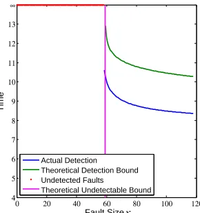
Figure 3.2 Comparison between actual and theoretical detection times, undetectable faults, and the theoretical undetectable fault bound. . . 35

Figure 3.3 Absolute detection time error. . . 36

Figure 3.4 First component of the residualr1 forκ= 117. . . 36

Figure 3.5 First component ofr1 for fault f2. . . 37

Figure 3.6 First component ofr1 for fault f3. . . 38

Figure 3.7 No response in second component ofr1 for both f3 and f4. . . 38

Figure 3.8 All components of r2 for piecewise constant fault f2. . . 38

Figure 3.9 All components of r2 for ramp fault f2 with ramp time 1/8. . . 39

Figure 3.10 All components of r2 for ramp fault f2 with ramp time 4. . . 39

Figure 3.11 Comparison between actual and theoretical detection time, undetectable faults, and the theoretical undetectable fault bound forf3. . . 40

Figure 3.12 Comparison between actual and theoretical detection time, undetectable faults, and the theoretical undetectable fault bound forf2. . . 40

Figure 3.13 First component ofr1 withκ= 105 andγ2. . . 41

Figure 3.14 Behavior of filters constructed using Prop. 3.3.2 forf1. . . 41

Figure 3.18 Behavior of filters applied to a linear combination f(t) =κ1f1(t) +κ2f2(t). . 43

Figure 3.19 Upper and lower bounds for κi. . . 44

Figure 3.20 Residual before (blue) after (green) disturbance filtering. . . 44

Figure 3.21 Fault identification filters applied to filtered residual. . . 45

Figure 4.1 Minimal properu for theL2 _{bound–Example 1.} _{. . . 73}

Figure 4.2 Minimal properu for theL2 _{bound–Example 2.} _{. . . 75}

Figure 4.3 (Run 1) (a) Random noises,µ1,η1 (b)Wi(t) and γ2. . . 77

Figure 4.4 (Run 2) (a) Random noises,µ1,η1 (b)Wi(t) and γ2. . . 77

Figure 4.5 A two-link robot arm with the second joint elastic, from [27]. . . 79

Figure 4.6 Comparison of numerically computed minimal proper signalsump, the signal for models 0 and 1, and uK, the signal for models 0 and 2, on [0 1]. . . 84

Figure 4.7 Comparison of numerically computed, minimal proper signals ump and uK on [0 10]. . . 84

Figure 4.8 (a) Proper auxiliary signal separating models 0 and 1 withγ = ₇₀1. (b)Wi(t) and γ2_{. . . 87}

Figure 4.9 Computed test signal for Example 4.7.1 on iteration 20 usingkuk2 2. . . 94

Figure 4.10 Minimal test signal for Example 4.7.1 using (4.73) with α= 0.1. . . 99

(11)

Figure 4.15 α vs.ku0

αk22 for Example 4.7.1. . . 102

Figure 4.16 Minimum proper test signal for modified Example 4.7.3 withu0 _{appearing in} the output. . . 103

Figure 4.17 kuk2 α,kuαk22,ku0αk22 for modified Example 4.7.3 plotted againstα. . . 103

Figure 4.18 Minimal proper test signals for Test 1. . . 111

Figure 4.21 Norm of minimal proper test signals for different r in Test 4. . . 113

(12)

Chapter 1

Introduction

Fault detection and identification (FDI) are important in almost all real systems. Fault detection is the supervision of technical processes aimed at detecting undesired or unpermitted states and

taking appropriate actions to avoid dangerous situations, or to ensure efficiency in a system.

Deviations from nominal behavior that are large enough to cause undesired states, even in robustly controlled systems, are known as faults. The task of fault identification is to determine

various characteristics of the fault, such as its type, size, or location.

The simplest and most common form of fault detection is known as limit checking [43]. Measured variables are checked with regard to tolerances, and alarms are generated for the

operator. Tolerances are determined from compromises between detection size and unnecessary

alarms. The simplicity of limit checking makes it an attractive option in many systems. Limit checking is effective in systems that operate approximately in a steady state, but may be

inaccurate if the system is rapidly changing. Limit checking may also be inadequate in the case

of a gradually increasing (incipient) fault or in systems under closed loop feedback because reaction occurs only after a relatively large change. In either case, faults may be masked until

the situation is catastrophic.

Another option is the use of hardware redundancy, where measurements from multiple sensors are compared with each other and a voting mechanism is employed to detect faults.

However, some applications may not permit the use of redundant sensors due to the extra cost,

weight, volume, etc., they require. In other situations, such as with actuators, direct measure-ments are often not possible or are prohibitively expensive, either practically or financially.

Therefore, advanced methods of fault detection have been developed with the goal of early,

reliable detection.

This thesis focuses on model-based approaches, i.e., approaches where mathematical models

(13)

work investigates observer-based approaches [33, 42, 70] and multiple-model detection [20].

Model-free approaches also exist, but are not the subject of this work [48]. Model-free ap-proaches are generally data driven and depend on statistical techniques to determine if a fault

has occurred. For example, anomaly detection uses data to find patterns that do not conform to

expected behavior [23]. Descriptive statistics are estimated from data generated by a system op-erating nominally. Then, given new data from a similar system whose operation is being tested,

it is possible to calculate the probability of the new data coming from a nominal system. One

advantage to statistically driven approaches is the ease with which they can deal with stochastic noise as opposed to the deterministic noise in this work. However, statistical approaches often

require further investigation once an anomaly is flagged. Model-based approaches, especially

those in this work, often yield much more information upon detection of a fault. Some sophisti-cated fault detection approaches use a combination of model-based and model-free approaches.

For a comprehensive overview of these approaches, both model-based and model-free, see [44].

Every FDI method can be classified as either passive or active. In the passive approach, measurements from the system are continuously monitored and compared to the normal

be-havior of the system in some way. Most work in FDI is based in this class of methods. The

observer-based approach in Chapter 3 is passive. Passive approaches are particularly useful for systems where auxiliary signals may pose a safety risk. The main disadvantage is that robust

control schemes may hide failures during normal operation.

Active methods, on the other hand, interact with the system to improve detection. Usually,

a test signal, constructed to highlight faults, is fed into the system, either on a test interval,

or on a periodic basis. We call this test signal the auxiliary signal and its construction is the subject of the early sections in Chapter 4. An elementary example of an auxiliary signal is

checking the brakes of a car while driving down a road, before they are needed. The auxiliary

signal is usually determined in advance, based on the given system, and is constructed with the specific intent of exposing faults. In some scenarios, a sequence of test signals is applied, each

one aimed at exposing a certain fault, or group of faults.

1.1 Differential Algebraic Equations

This dissertation develops new, or in some cases extends, fault detection techniques for

sys-tems modeled by differential algebraic equations (DAEs). A system F(x0(t), x(t), u(t), t) = 0 is, in general, a system of DAEs. If Fx0_(t) is nonsingular, then it is a system of ordinary

dif-ferential equations (ODEs), a class of equations subsumed by the class of DAEs. The methods

(14)

from this point forward we will use the term “DAE” in place of “higher index DAE” to indicate

a set of differential equations which are not an ODE.

DAEs arise naturally in many applications, especially in applications with a need for fault

detection and identification. Some examples include electrical circuits, trajectory prescribed

path control, systems of rigid bodies, problems in constrained mechanics, electrical networks and chemical reactions [10]. A classical example of a DAE arising from a constrained mechanical

system with positionx, velocityv, kinetic energyT(x, v), external forcef(x, v, t) and constraint

φ(x) = 0 is

∂2_T

∂v2v

0 ₌_g₍_{x, v, t}_{) +}_GT_λ _(1.1a)

x0 =v (1.1b)

0 =φ(x), (1.1c)

where G = ∂φ_∂x, and λ is the Lagrange multiplier. The constraints (1.1c) make this system a

DAE, not an ODE, even if ∂_∂v2T2 is invertible. If it is invertible, multiplication of (1.1a) by ∂ 2_T

∂v2 −1 converts (1.1) into a semi-explicit DAE.

DAEs differ from ODEs in several key aspects. The singularity conditions onFx0 mean DAEs

always contain pure algebraic equations called constraints like equation (1.1c). In terms of fault detection, this will be advantageous because it will allow additional residual information to be

considered when looking for faults. However, not all constraints are given explicitly and some

are even hidden constraints. Hidden constraints are only visible after differentiating the given equations. For example, consider the following semi-explicit DAE,

x0₁+x3 =f1 (1.2a)

x0₂+x1 =f2 (1.2b)

x2 =f3 (1.2c)

where xi are the unknowns and fi are external forcing terms. The fi may even be faults or disturbances in the problem. Equation (1.2c) is the only explicit algebraic constraint. However,

a few differentiations and substitutions result in finding the only solution to this DAE,

x1=f2−f30 (1.3a)

x2=f3 (1.3b)

x3=f1−f20 +f

00

(15)

because there are two additional implicit algebraic constraints in the original DAE. Note the

derivatives of the faults or forcing terms appear in the solution of the DAE. This is unlike the situation for ODEs and will have consequences for fault detection as we will see later (Section

3.6.2). Depending on the specific situation, the presence of fault derivatives can make the fault

harder or easier to detect than in the analogous ODE case. If the fi represent unavoidable disturbances as a result of normal operation of the system, (1.3) exposes the full impact that

disturbances will have on the system. To be specific, even small disturbances will have large

impacts on the system if their derivatives are large.

There are also numerous numerical difficulties associated with working with DAEs that are

not present with ODEs [10]. The presence of algebraic constraints cause the solutions of a DAE

to form a manifold called the solution manifold. Only the initial conditions that lie on the solution manifold accept a solution to the DAE. These are called consistent initial conditions.

This characteristic of DAEs suggests that a they can be thought of as an ODE defined on

a solution manifold. Therefore, numerically solving a DAE amounts to solving an ODE with constraints whether they be implicitly or explicitly defined.

1.2 Observer-Based Approach

In Chapter 3, we develop a passive FDI approach for systems modeled by DAEs based on the

use of observers to estimate the true state of the system. The observer is used to generate an

output error, also known as the residual, and faults are detected if the output error is far enough from zero. To illustrate, let us begin with the linear time invariant (LTI) ordinary differential

equation (ODE) model with output

x0(t) =Ax(t) +Bu(t) +fp(t)

y =Cx(t) +fs(t)

whereu(t) is the control,fp(t) is a process fault, andfs(t) is a sensor fault. Iffp =fs= 0, then

the system is operating normally. Suppose we design an observer, e.g., the standard Luenberger

observer

ˆ

x0(t) =Axˆ(t) +L(y(t)−yˆ(t)) +Bu(t) ˆ

(16)

such that the dynamics of the state estimation error, e(t) = x(t)−xˆ(t), are asymptotically

stable. The dynamics of the state estimation error are

e0(t) = (A−LC)e+fp(t) +Lfs(t),

so in the LTI case, this simply means A−LC is asymptotically stable. Then, in the absence of

faults, the state error vanishes asymptotically

lim

t→∞e(t) = 0.

Define the output error, or residual, to be r(t) = y(t)−yˆ(t). y(t) are the measured outputs from the system and ˆy(t) are the outputs generated by the observer. Hence, both are available

for our purposes. If there are no faults, r(t) approaches zero as the state estimation error goes

to zero. One way to make a decision on faults, is to create a problem dependent threshold,τ, and compare τ to r(t).τ could be a vector of the same length as r(t) or a positive number. If

τ is a number one might say a fault is detected ifkr(t)k> τ. An example of a decision-making comparison when τ is a vector is the following: if ri(t) > τi, in any component i, then a fault is detected. The approach in Chapter 3 is a modified version of this approach, so that it is

applicable to DAE systems.

Other previous work in observer-based fault detection in ODEs has also included the design of unknown input observers [24], dynamically extended observers [70], descriptor observers [33],

and sliding mode observers [22, 47]. These works are applicable to linear ODE models. On the

other hand, the authors of [34] and [73] construct observers for nonlinear systems, but a formal method of applying these observers to fault detection is absent.

1.3 Fault Detection in DAEs

Previous work on FDI in DAEs has included the idea of model-based fault diagnosis for

discrete-time descriptor linear parameter varying (LPV) systems. LPV systems are a special case of LTV systems. The authors of [3] provide sufficient conditions to ensure the existence and the

stability of the proposed observer by using a combined Lyapunov analysis based on a linear

matrix inequalities formulation. While the LPV assumption may simplify the process of FDI in the DAE systems that meet this assumption, it does not lend itself to developing general

methods. Our work on observer construction for FDI, while initially developed for LTI systems,

is potentially applicable to general DAE systems including the general LTV and nonlinear cases. Previous work, first in [71] and later refined in [26] (also developed independently and in

a slightly different manner in [72]) constructs unknown input observers using a sliding mode

(17)

directly applied to the DAE without any reduction or reformulation. This requires certain

assumptions on the matrices of the LTI DAE that are different than our assumptions for the construction of an observer. In general, unknown input observers require the regularity of a

certain matrix pencil [10], computation of more matrices than the one gain matrix commonly

found in the design of observers for LTI ODE, and rely on eigenvalue placement techniques. These dependencies make it difficult to generalize these observers for LTV and nonlinear DAE

systems. In addition, the authors of [30] introduce a descriptor unknown input observer with

sliding modes. This introduces the added complexity of simulating a descriptor system in order to obtain state estimates.

However, an advantage of the sliding mode approach, in addition to the simplicity of not

requiring any reformulation, is the ability to follow the behavior of the faulty system. The mechanism of detection is based on monitoring abnormal deviations of the controlled outputs

from their the set point trajectories and deviations of the estimated parameters from their

nominal values. Moreover, disturbances are easily decoupled with unknown input observers by assuming the fault and disturbance enter the system with different distribution matrices. In

Section 3.4 we give an alternative approach based on the discrete Fourier transform that does

not require this assumption.

Articles [39], [40], and [45] develop techniques for parameter estimation in DAE. Paired

with a decision making threshold for the difference between parameter estimations and nomi-nal values, parameter estimation can be made into a passive fault detection approach. While

the estimates provide a powerful FDI technique, the approach in [40] and [45] also requires

the solution of a nonlinear programming problem, certainly a nontrivial task, and potentially computationally expensive. While appropriate for some applications, the time-sensitive nature

of fault detection may prohibit these methods. In general, parameter estimation for DAE has

yet to be formalized for the specific purpose of FDI.

A large percentage of this thesis concerns itself with active detection in DAEs. Since previous

work in active detection has only been developed for systems modeled by ODEs, the related

methods in this thesis are pioneering ideas in this field. Due to the absence of competing methods, in the following we summarize previous active detection work for ODE systems.

In some ways, the auxiliary design methods developed in this thesis can be seen as the

DAE analogs to the methods developed by the authors of [20] and [54] for ODEs. These works employ a multi-model approach, meaning there are at least two models, one for the nominally

operating system, and the others for the faulty systems. In these works, dynamic optimization

is used to find the smallest auxiliary signal that guarantees fault detection by constructing a small signal that forces the output sets to be disjoint, even in the presence of bounded noise. It

(18)

an optimal control problem, is computed offline, and then applied to the system. The measured

outputs which, by construction, can only come from one of the models, are monitored during the test interval and a decision is made, possibly before the end of the test period. The approach

has since been extended for detection of incipient faults [53], to include a priori information

about the initial condition [52], the presence of model uncertainty [1], and for nonlinear systems [2], [68].

The authors of [61] develop an alternative method of constructing an auxiliary signal that

is based on a moving horizon for discrete time systems. That is, instead of pre-computing the test signal, online measurements during the test interval are used to refine an open-loop input,

initially computed offline. In general, moving horizon approaches have the potential to produce

much more conservative inputs (e.g. reduced duration, norm, etc.). In [61], the initial optimal input is computed by solving an expensive mixed-integer quadratic program. Then, at each

time step, the optimal input is recalculated by solving this problem using updated information

from system measurements. The authors note the computation time required for this method makes it impractical for many applications of interest. To address this, they develop a much

more efficient method by computing all possible reachable sets offline and storing them. An

optimal input strategy is computed for each possible trajectory, stored in a table, and at each time step, the optimal signal for that time step is selected. The main drawback to this approach

is that it requires very strict assumptions. The authors assume the matrix coefficient on the state in the output for each model is invertible and they restrict the set of possible noises. Even

the basic method, which is too computationally expensive for online usage, requires restrictive

assumptions including the following: the control lies in a convex polytope, the noises are zero-centered zonotopes, the initial states lie in zonotopes, and the faults are time invariant.

In [50], the author extends fault detection results from closed loop systems to open loop

systems, as well as closed loop systems with feedback controllers. The open loop system is derived from the closed loop system by removing the feedback controller. A transfer function

matrix is derived between the input and the residual vector that is equivalent to the fault

signature matrix in the closed loop case. This shows that it is possible to use the same active fault detection method on the closed and open loop systems. The only restriction being the

maximal number of faults occurring simultaneously is bounded by the number of control signals

minus one.

1.4 Thesis Outline

Although work on FDI in systems modeled by DAE is not new–the approaches in previous paragraphs are such examples–there are relatively few works in the area, compared to ODE

(19)

In Chapter 2 we reformulate the DAE problem using the completion technique–described later

in Section 2.2–and derive some properties related to it in Section 2.4. In Chapter 3 we use the completion to construct an observer, compute outputs based on the observer, and construct

residuals to make decisions on fault detection. We also develop linear filters to identify faults

and address disturbance attenuation using the discrete Fourier transform. We apply this method to a DAE circuit model and illustrate its benefit in Section 3.6.

In Chapter 4, we turn to the task of active detection. Analogous work on ODE models is done

in [20]. Since DAE are singular, the standard techniques for FDI in the ODE case are not directly applicable to the DAE case. A reformulation of a bi-level optimization problem with DAE

constraints is necessary to construct a problem that can be implemented using modern software.

A novel theorem is presented to identify the active model in real-time. We also investigate some shortcomings of the method in Chapter 4 and present a suboptimal modification. Finally, we

investigate a related topic in auxiliary signal design known as asynchronous active detection, a

strategy where the output is watched on a different time interval than the interval the auxiliary signal is applied on. We show the result is a cheaper test signal and sometimes a shorter test

interval.

(20)

Chapter 2

Background

In this chapter, we summarize the theory of completions, originally introduced in [14], and later matured in [13], [56], [57], [17], [18], and [55]. A completion of a DAE is an ODE whose solutions

include those of the DAE. The specific type of completion studied here, and in the references

herein, is known as the least squares completion, so named because after constructing a large set of equations, known as the derivative array, the state is solved in the least squares sense.

The least squares completion has been developed for general DAEs with no necessary structural

assumptions, originally as part of a general numerical solution technique. The generality of the method makes our FDI approach potentially applicable to systems modeled by general DAEs.

The completion procedure generates an ODE containing the solutions of the DAE. The

extra solutions, known as the additional dynamics, have been shown to be stable, provided some care is taken [55]. In that case, the completion is known as the stabilized completion. As

shown in Section 3.1, this enables us to construct a Luenberger observer for the completion and

rely on its state estimates to generate residuals for fault diagnosis.

2.1 DAE Preliminaries

Recall, we are assuming the systems under consideration may be approximated by models of the form

F(x0(t), x(t), u(t), t) = 0, (2.1) wherexis the state,uis the control, bothF andxare vector valued, andFx0(x0(t), x(t), u(t), t) is singular. In what follows, we are concerned with the case where the solutions exist and are

uniquely defined on the interval of interest. Unlike ODEs, not all initial values for x admit a smooth solution; those that do, are called consistent initial conditions. Intuitively, a system of

DAEs is solvable if the system’s solution is determined by a consistent initial condition. A more

(21)

Definition 2.1.1. Let I be an open subset of R, Ω a connected open subset of R2m+1_{, and} _F a differentiable function for Ω to Rm_{. Then the DAE} _(2.1) _is_solvable _on_I _in _Ω_{if there is an}

r-dimensional family of solutions φ(t, c) defined on a connected open set I×Ω˜,Ω˜ ⊂ Rr_{, such} that

1. φ(t, c) is defined on all ofI for each c∈Ω˜

2. (φt(t, c), φ(t, c), t)∈Ω for (t, c)∈I×Ω˜

3. If ψ(t) is any solution with(ψ0₍_t₎_{, ψ}₍_t₎_{, t}₎_∈_{Ω, then} _ψ₍_t_{) =}_φ₍_{t, c}₎ _{for some} _c_∈_Ω_˜

4. The graph of φ as a function of (t,c) is an (r+ 1)-dimensional manifold.

The definition says that there is a local, r-dimensional family of continuous solutions with

no bifurcations, on the interval I. The definitions and theorems in this section, including the

previous definition, can be found in [10].

A useful property when discussing completions is the index of the DAE. The index plays

a key role in the classification and behavior of DAEs. In order to motivate the definition that

follows, consider the special case of a semi-explicit DAE

x0 =f(x, y, t) (2.2a)

0 =g(x, y, t). (2.2b)

If we differentiate the constraint equation (2.2b) with respect to twe get

x0 =f(x, y, t) (2.3a)

gx(x, y, t)x0+gy(x, y, t)y0 =−gt(x, y, t). (2.3b) If gy is nonsingular, the system (2.3) is an implicit ODE and we say that (2.2) has index one.

If this is not the case, suppose with coordinate changes we can rewrite (2.3) as (2.2), but with

different x, y. Then, we repeat the differentiation and coordinate changes until we can get to an ODE. The number of differentiations required in this procedure is known as the index. For

example, a DAE of index zero is an ODE.

Definition 2.1.2. The index, k, of a system of DAEs is the minimum number of times the system is differentiated with respect to t in order to uniquely determine the first derivative of the state vector as a continuous function of the state vector and t.

Suppose we differentiate (2.2) with respect tot,ktimes, wherekis the index. Then we have

(22)

d

dtF = 0 (2.4b)

.. .

dk

dtkF = 0, (2.4c)

which together are known as the derivative array and are denoted byG(z, x, t), where

z(t) = 

  

x0(t) .. .

x(k+1)₍_t₎ 

  

For a linear DAE, such as

E(t)x0(t) +F(t)x(t) =B(t)u, (2.5) the derivative array is

E(t)z(t) +F(t)x(t) =B(t)¯u(t), (2.6)

where E =         

E 0 0 . . . 0

E0+F E 0 . . . 0

E00_{+ 2}_F0 ₂_E0₊_F _{E . . .} ₀

.. . . .. ... . . . .         

, F =

         F F0 F00 .. . F(k)          .

B = diag(B, B, . . . , B) and ¯u defined in an analogous way to F, except for vectors. Upon

consideration of the derivative array, we have the following convenient definition:

Definition 2.1.3. Theindex, k, of a linear system of DAEsE(t)x0(t) +F(t)x(t) =B(t)u(t)is the minimum number of times the system is differentiated with respect totso that the coefficient

matricesE(t),F(t)from the derivative array equationsE(t)w(t) +F(t)x(t) =B(t)¯u(t)meet the following conditions:

1. h

E(t) F(t) i

is full row rank for all t;

2. E(t) has constant rank; and

3. if x(t) isn dimensional, thenE(t)b(t) = 0 for some vector b(t) implies the first n entries for b(t) are zero for allt.

(23)

2.2 Completion Theory

A completion of

E(t)x0(t) +F(t)x(t) =B(t)u(t) +fp(t), (2.7) a linear system of DAEs, with possible faults fp, is a linear system of ODEs

x0(t) = ˆA(t)x(t) + ˆB(t)¯u(t) + ˆG(t) ¯fp (2.8) designed so the solutions of (2.8) contain those of (2.7). For any vector functionq, we use ¯q to denote a vector containing q and the firstk−1 derivatives ofq with respect tot. As discussed

in the introduction, for an n-dimensional system of linear DAEs, solutions are defined on the

less thenn-dimensional solution manifold. Since (2.8) is ann-dimensional ODE, there exists an

n-dimensional family of solutions. Therefore, there are extra solutions whose behavior will be discussed in what follows.

Recall we denote the derivative array, given by (2.4), asG(z, x, t). We will need the following definition [12]:

Definition 2.2.1. A system of algebraic equations

A

"

x1

x2 #

=b (2.9)

is called 1-full with respect to x1, ifx1 is uniquely determined for any consistent b.

Suppose the following assumptions are satisfied for bothkandk+ 1 in some neighborhood:

I. Sufficient smoothness of G= 0.

II. G= 0 is consistent as an algebraic equation.

III. Gz is 1-full and has constant rank independent of (z, x, t).

IV. h

Gz Gx i

has full row rank independent of (z, x, t).

When these assumptions are met, then multiplication by the Moore-Penrose inverse [19], E†_,

solves uniquely forx0

x0(t) =−E†Fx+E†Bu¯+E†f¯p

and determines the least squares completion (2.8) where ˆA, ˆB, and ˆGare the first block row of

(24)

Assumptions I.-IV. also imply the geometric solvability of the linear DAE [16], a notion

related to the solvability definition found in this thesis. Having no need for geometric solvability here, for our purposes these assumptions are only required for the calculation of the completion.

Thus far, to form the derivative array, we differentiate the system of DAEs k times, where

k is the index of the DAE. However, it has been shown in [56] the additional dynamics may be unstable, leading to numerical inaccuracies. Therefore, we modify the approach by applying

the differential polynomial D = _dtd + Λ instead, where Re(s) > 0 for all eigenvalues s of the

matrix Λ. The authors of [17] have shown this modification stabilizes the additional dynamics and guarantees no repeated eigenvalues in the additional dynamics. Repeated eigenvalues make

construction of observers problematic unless there are sufficient outputs.

As a first step in fault detection, this thesis considers LTI DAEs

Ex0+F x=Bu+fp. (2.10)

Therefore, in the following, we demonstrate the construction of the derivative array and calcu-lation of the completion using D on LTI systems. Applying D to (2.10) k times results in the

modified derivative array

DjE "

x0 ω

#

=−DjFx+DjBu¯+Djf¯p (2.11)

where E =         

E 0 0 . . . 0

F E 0 . . . 0

0 F E . . . 0

.. .

0 0 . . . F E

        

, Dj =         

I 0 0 . . . 0

Λ I 0 . . . 0

Λ2 2Λ I . . . 0

..

. . ..

Λk _k_Λk−1 _{. . . I}          ,

F =hFT ₀ ₀ _{. . .} ₀iT _, _and_B_{= diag}_{_{B, B, . . . , B}_}_.

DjE is rank deficient. For many classes of DAEs, such as the Hessenberg DAEs of mechanics, ˆ

Bu¯ involves none or one derivative ofu.

Suppose assumptions I.-IV. are satisfied for both kand k+ 1 in some neighborhood. Then

solving (2.11) in the least squares sense we get

ˆ

(25)

other components of ˆzwill usually not be the higher derivatives ofx and will be ignored. Thus

taking the first block row of (2.12) we get the least squares completion

x0 = ˆAx+ ˆBu¯+ ˆGf¯p. (2.13) The constraints

0 =Gx+ ˜Bu¯+ ˜Gf¯p (2.14)

are found by multiplying (2.11) by a maximal rank left annihilatorU ofDjE. We partition ˆGand ˜

Gconformal with ¯fp so that ˆG= h

ˆ

G0, . . . ,Gˆk−1 i

. Iffp is constant, then ¯fp=

fT

p ,0, . . . , 0 T

so that only ˆG0 is needed. The ˜Gi notation is similar. The constant fault case happens often

enough to warrant this consideration.

2.3 LTI Systems

LTI systems have some properties that we will exploit in the following sections. First, we will

need the following definitions and theorems.

Definition 2.3.1. The matrix pencil for the linear time invariant system of DAEs in (2.10) is sE+F for a complex scalars.

Definition 2.3.2. The finite generalized eigvenvalues of the system in (2.10) are all s such thatdet(sE+F) = 0.

Finite generalized eigenvalues play the same role for (2.10) that regular eigenvalues do for

LTI ODEs. That is, if u(t) = 0 and λ is one finite generalized eigenvalue of (2.10), then one

mode of the solution iseλt_.

Definition 2.3.3. If the determinant of sE+F, denoted det(sE+F) is not identically zero as a function of s, then the pencil is said to be regular.

In general, the solvability of a general DAE can be difficult to determine; however, for (2.10) there is a nice characterization. The next theorem explores the relationship between the

solvability of the LTI DAE and its matrix pencil.

Theorem 2.3.1. The linear constant coefficient DAE is solvable if and only if sE+F is a regular pencil.

(26)

Theorem 2.3.2. Suppose thatsE+F is a regular pencil. Then there exist nonsingular matrices

P, Q such that

P EQ=

"

I 0

0 N

#

, P F Q= "

C 0

0 I

#

(2.15)

where N is a matrix of nilpotency k and I is an identity matrix. If N = 0, then define k= 1.

In the special case that E is nonsingular, we take P EQ=I, P F Q=C, and define k= 0. If

det(sE+F) is identically constant, then (2.15) simplifies toP EQ=N,P F Q=I.

The degree of nilpotency,k, is the same as the index of the DAE.

2.4 Useful Facts about Completions

Given a LTI DAE the least squares completion is a LTI ODE with LTI constraints. This

section gives some useful results about the matrices computed by the completion procedure. In the following discussion we apply a similarity transformation to arrive at a simpler DAE. We

will prove certain properties that completions of this simpler DAE possess and extend them to

the completion of (2.10) via their relationship by a similarity transformation.

Suppose the matrix pencil sE +F is regular. Then, by Theorem 2.3.2, there exists an

orthogonal P and a nonsingular Qsuch that

P EQ=

"

C1 C2

0 N

#

, P F Q= "

D1 D2 0 D3 #

(2.16)

where C1 and D3 are invertible and N is nilpotent of the same degree as the index of (2.10).

Therefore, left multiplication by the orthogonal matrixP and the coordinate change given by

x=Q

"

y1

z2 #

transforms the DAE into

C1y10 =−C2z20 +D1y1+D2z2+f1

N z₂0 =D3z2+f2.

where D₃−1N is nilpotent. Then, using the transformation y2 = D3−1z2 and relabeling coeffi-cients, we obtain the system

C1y01=−C2y20 +D1y1+D2y2+f1 (2.17a)

N y0₂=y2+f2. (2.17b)

(27)

additional restriction that P is orthogonal instead of just nonsingular to obtain a relationship

between the completions of (2.10) and (2.17).

Since C1 is nonsingular, (2.17a) is index zero. Then, the completion of (2.17) is (2.17a)

and the completion of (2.17b). The following proposition [57], will be helpful in finding the

completion of (2.17b).

Proposition 2.4.1. Suppose the LTI DAE in (2.10)is solvable with indexk and its derivative array is given in (2.11). Suppose that assumptions I.-IV. are satisfied for this system. Let G0

be an n×(k+ 1)n matrix satisfying G0DjE = h

I 0 . . . 0 i

and G0Z = 0, where Z is a

matrix of maximal rank satisfying ZT_D

jE = 0. Namely, the columns of Z form a basis for the null space N(ET_DT

j ). Then, the least squares completion of (2.10) defined by (2.11) is

x0 ₌_G

0Dj(−Fx+Bu¯+ ¯fp).

In particular, this means given DjE "

y0

2

ω

#

=Dj(−Fy2+ ¯f2), the derivative array of (2.17b),

we get the completion

y0₂=−G0DjFy2+G0Djf¯2 = ˆA2y2+ ˆG2f¯2. (2.18) If the fault is constant, we look at ˆG20 =G0D0 whereD0 is the first block column ofDj. Note

that in this caseF =−I, so−G0DjF =G0D0 and ˆA2 = ˆG20. Therefore ˆG20 is invertible since

ˆ

A2 is invertible from [57]. We will need this fact later. Proposition 2.4.1 leads us to the following

Lemma 2.4.1. The stabilized least squares completion for (2.17b) is given by (2.18) and the matrices in (2.18) satisfy G2Aˆ−21Gˆ20 −G˜20 = 0.

Proof. We know that (2.18) is the least squares completion of (2.17b) and ˆA2 is invertible. The lemma now follows because

G2Aˆ−21Gˆ20−G˜20 =U

      I λI λ2_I

.. .      

I−U

      I λI λ2_I

.. .      

= 0.

Equation (2.17a) is index zero so it is invariant under the least squares completion process. Thus, there are no constraints associated with (2.17a). Using the truncated versions of ˆG and

˜

(28)

0 =G1y+ ˜G10f (2.19b)

whereG1 = h

0 G2 i

, ˜G10 =

h 0 G˜20

i and

ˆ

A1 = "

C₁−1D1 ∗ 0 Aˆ2

#

, Gˆ10 =

"

∗ ∗

0 Gˆ20

#

(2.20)

letting∗denote nonzero blocks. The next lemma extends Lemma 2.4.1 to the entire completion of (2.17). In the proof of the next lemma, we assume 0 is not a finite eigenvalue of (2.10) since

we will subsequently need to assume this for the purposes of fault detection.

Lemma 2.4.2. The matrices in (2.19)satisfy G1Aˆ1−1Gˆ10−G˜10 = 0.

Proof. C1is invertible by assumption. ˆA2 is invertible from [57]. Then ˆA1is invertible as defined

in (2.20) since 0 is not a finite eigenvalue of (2.10). ConsiderG1Aˆ−₁1Gˆ10−G˜10. This is equivalent

to

h 0 G2

i "

∗ ∗

0 Aˆ−₂1

# "

∗ ∗

0 Gˆ20

#

−h0 G˜20

i =

h

0 G2Aˆ2Gˆ20 −G˜20

i

.

An application of Lemma 2.4.1 completes the proof.

Finally, we connect the transformed system in (2.17) and the original system (2.10) with

the following

Lemma 2.4.3. Consider the original system (2.10) and its stabilized least squares completion (2.13)–(2.14). Then GAˆ−1_Gˆ₀₋_G˜₀ _{= 0.}

Proof. In [57], it was shown that given the original system and its completion, the corresponding completion of (2.17) is

y0 =Q−1AQyˆ +Q−1Gˆ0f¯ (2.21a)

0 =GQy+ ˜G0f¯ (2.21b)

if we redefineQ=Q

"

I 0

0 D−₃1

#

. Lemma 2.4.2 implies that (GQ)(Q−1_Aˆ−1_Q₎₍_Q−1_Gˆ₀₎₋_G˜₀ _{= 0.} The current lemma follows because (GQ)(Q−1_A_ˆ−1_Q₎₍_Q−1_G_ˆ

0)−G˜0 =GAˆ−1Gˆ0−G˜0. Recall ˆG20 is invertible. We can now prove the following

(29)

Proof. Since (2.17a) is invariant under the stabilized least squares process we have ˆG10 =

"

C₁−1 −C₁−1C2Gˆ20

0 Gˆ20

#

which is invertible. Equation (2.21) implies ˆG0 = QGˆ10, a product of

invertible matrices.

(30)

Chapter 3

Observer-Based Passive FDI

3.1 Observer Construction

As a first step in fault detection, this thesis considers LTI DAEs with outputs and possible process and sensor faults, fp and fs,

Ex0+F x=Bu+fp (3.1a)

y=Hx+Du+fs. (3.1b)

We assume E, F are square matrices, E may be singular, u is a known control input, fp is a process fault, fs is a sensor fault, there is a scalars for whichsE+F is invertible—that is,

{E, F} form a regular matrix pencil so that (3.1a) is solvable—xand uare functions of time t,

x is n×1,y ism×1, and 0 is not a finite eigenvalue of the pencil sE+F. If we also assume assumptions I.-IV. are met, then we can compute the stabilized least squares completion with

output,

x0= ˆAx+ ˆBu¯+ ˆGf¯p (3.2a) 0 =Gx+ ˜Bu¯+ ˜Gf¯p (3.2b)

y=Hx+Du+fs. (3.2c)

We construct a Luenberger observer that is unaware of the faults and ignores (3.2b) so that it

takes the form

ˆ

x0= ˆAxˆ+L(y−yˆ) + ˆBu¯ (3.3a) ˆ

(31)

where the eigenvalues of ˆA−LH are designed to give us the desired convergence rate of the

observer. If{A, Hˆ }is not completely observable, then we need the unobservable eigenvalues to have negative real part. If they are not finite eigenvalues of the matrix pencil sE+F, then

they are from the stabilization parameter matrix Λ and are user specifiable. Observability of

(3.1) does not imply the observability of (3.3) unless (3.2b) is viewed as an extra output. Such reduced order observers are considered in [7, 8] but are outside the scope of this work.

Let e=x−xˆbe the observer error. Then,

e0 = ( ˆA−LH)e−Lfs+ ˆGf¯p (3.4a)

y−yˆ=He+fs. (3.4b)

Using our outputs, observer estimate ˆx, and information on the solution manifold (3.2b), we

have two residual vectors available to us instead of the usual one,

r1 =y−yˆ (3.5a)

r2 =Gxˆ+ ˜Bu.¯ (3.5b)

Both of these residuals should be zero if the observer has converged (that is, the estimation

error is less than some tolerance) and there are no faults. We shall assume the observer error

bound takes the form,

kh(t)k ≤βeα(t−t0)₊₌_θ₍_t₎_, _(3.6)

for β > 0, > 0, and α < 0, where t0 is the start time of the fault. Here α comes from the theoretical convergence rate of the observer and models numerical, measurement, and other

small but nonzero errors. The constant β is a bound on the size of disturbances due to either

the onset of the fault or by other disturbances to the system. θis to simplify some expressions later.

3.2 Detection

As is often done in the literature, we assume that once fully developed the fault is constant

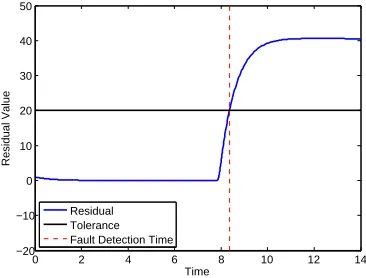
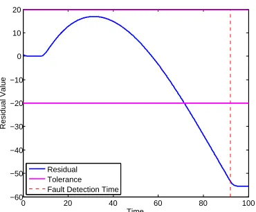
and in a particular direction. As we will see later, with DAEs, the start up of the fault can

play a larger role in detection than in the case of ODE systems. Certain faults can be more easily detected if they occur quickly as shown with the circuit example in Section 3.6. Thus, we

assume faults take the form

(32)

g(t) is a monotonically non-decreasing, smooth function that is zero for t ≤ t0 and one for

t≥t1. On the interval [t0 t1], it takes the form g(t) =c(t−t0)2+d(t−t0)3. Constants c and

d are determined with the conditions g(t1) = 1 and g0(t1) = 0. If t0 = t1 then the fault is a piecewise constant, abrupt fault and there is no transient period. Otherwise, the fault appears

in a smooth manner and is called a ramp fault.di is a constant vector andκis a scaling constant allowing us to discuss thresholds and detection times in terms of the size of the fault.

Note the smoothness of the fault is only assumed for purposes of analysis and in order to

simulate the fault. In practice, the fault does not appear in the observer equation and we use the real output y rather than a simulated output. Hence, we can detect most faults regardless

of their regularity.

We assume that ˆA−LH is invertible. The only time this might not be true in a case of interest is if we were designing dead beat observers for a discrete time system. This case will

be left for future work.

Using (3.2b), if we consider r2−0, we get

r1=He+fs (3.7a)

r2−0 =r2−(Gx+ ˜Bu¯+ ˜Gf¯p) (3.7b)

r2=−Ge−G˜f¯p. (3.7c)

After the initial ramp up interval of the fault and after the observer has converged, we have

e(t) =−( ˆA−LH)−1(−Lfs+ ˆGf¯p). The residuals can be expressed

r1=−H( ˆA−LH)−1(−Lfs+ ˆGf¯p) +fs+Hh

r2=G( ˆA−LH)−1(−Lfs+ ˆGf¯p)−G˜f¯p−Gh or the more condensed

W

" ¯

fp

fs #

+ "

H

−G

#

h(t) = "

r1

r2 #

. (3.9)

Letf =hf¯T p fsT

iT

and denote (3.9) by

W f+Qh(t) =r, (3.10)

whereW andW0 (to be used later) are

W =

"

−H( Â−LH)−1Gˆ H( Â−LH)−1L+I G( Â−LH)−1Gˆ−G˜ −G( Â−LH)−1L

#

(33)

W0 = "

−H( ˆA−LH)−1Gˆ0 H( ˆA−LH)−1L+I

G( ˆA−LH)−1Gˆ0−G˜0 −G( ˆA−LH)−1L #

(3.12)

and f0 = h

dT p dTs

iT

, where dp and ds are constant vectors determining the directions of the process and sensor faults, respectively.

Note thatW andW0are partly determined by the original system, partly by the stabilization

of the additional dynamics, and partly by the choice of L used in the design of the observer. If W0 6= 0, then generically most faults can be detected assuming the fault is large enough.

However, we want more detailed information on the size of the faultκand the time to detection.

There are different ways to evaluate residuals. One common way to do so is with element residual thresholds. These can be taken asymmetric but here we will say a fault is to be detected

if|ri|> τi for anyith component of the residual vector r and the user chosen threshold vector

τ which has positive entries. If a sufficiently large fault occurs andt > t1, then there is at least oneisuch that

|κ[W0f0]i+ [Qh(t)]i|> τi. (3.13)

Proposition 3.2.1. Suppose h(t) is bounded according to (3.6), t > t1 and

κ > τi+kQkβe

−α(t−t0)₊_k_Q_k |[W0f0]i|

(3.14)

for time t and some index i. Then (3.13) holds and thus, the fault f can be detected by timet.

Proof. Assumption (3.14) is equivalent to |κ[W0f0]i|> τi+kQkβe−α(t−t0)+kQk. Therefore, either

κ[W0f0]i > τi+kQkβe−α(t−t0)+kQk, or (3.15a)

κ[W0f0]i <−τi− kQkβe−α(t−t0)− kQk. (3.15b) The bound in (3.6) and (3.15) implies either

κ[W0f0]i> τi−[Qh(t)]i or

κ[W0f0]i<−τi−[Qh(t)]_i.

This is equivalent to

κ[W0f0]i+ [Qh(t)]i> τi or

(34)

The urgency of detecting the fault may vary from application to application; however, the

ability to detect the fault as quickly as possible is always a benefit. Suppose that (3.14) holds. Then it is clear that if

e−α(t−t0)_< |W0f0|iκ−τi− kQk kQkβ

the fault with scaling parameterκ can be detected by time t. Alternatively, we have

Proposition 3.2.2. If |[W0f0]i|κ−τi− kQk > 0, and t > t1, then detection can be done by time t if

t−t0 >− 1

α log

_|

W0f0|iκ−τi− kQk

kQkβ

. (3.16)

Now we turn our attention to the time varying aspect of the fault. Recallf in (3.10) is "

¯

fp

fs #

which includes the derivatives of fp. Then,

f =κ

     

g(t)dp

g0(t)dp

g00(t)dp

g(t)ds       . (3.17)

We have already analyzed the case when t > t1. Whent0 ≤t≤t1 a fault is detected if

κ       W      

g(t)dp

g0(t)dp

g00(t)dp

g(t)ds             i

+ [Qh(t)]i

> τi.

Then, analogously to (3.14), |ri(t)|> τi holds if

κ > τi+kQkβe

−α(t−t0)₊_k_Q_k

      W      

g(t)dp

g0(t)dp

g00₍_t₎_d

p

g(t)ds             i .

3.2.1 False Alarms

There is a trade-off when choosing the tolerance, τ, between permitting false alarms and de-tecting small faults. In some applications—especially in safety related processes like aircraft,

(35)

system. In other applications, it may be more cost effective to choose a higher tolerance so that

false alarms are a rare occurrence or never happen at all.

False alarms occur if the residuals cross the threshold set by the tolerance,τ, and f = 0 in

the equation

W f+

"

H

−G

#

h(t) = "

r1

r2 #

.

Then, ifτ is to be chosen to prevent this, it is necessary that

" H −G #

h(t) < τ

where<refers to component-wise comparison. Using (3.6), it is clear that ifτ is chosen so that

τ > " H −G #

βe−α(t−t0)_,

then no false alarms will occur.

3.2.2 Fault Location

Not all faults are treated equally because of the presence of the DAE. Let P = [(sE +

F)−1F]D[(sE+F)−1F] where D denotes the Drazin pseudoinverse [19]. ThenP fp enters the equations much like an ODE where (I −P)fp can contain derivatives. Thus if (I −P)fp = 0 we can treat it as an immediately occurring fault where as if (I−P)fp 6= 0 then there may be

transient reactions to the fault of increasing magnitude the quicker the fault occurs. Note that

N(G) =R(P). This is illustrated with the circuit example in Section 3.6.

3.3 Fault Identification

The task of fault identification consists of determining the type, size, and location of the detected fault. In this section, the idea of fault identification is narrowed to specifying which fault has

occurred given a library of possible faults. Consider process and sensor fault directions dpi

and dsi. Then, the fault can be written fi(t) = κ(g(t)v1i+g 0₍_t₎_v

2i+g 00₍_t₎_v

3i), where v1i =

[dT pi 0 0 d

T si]

T_, _v

2i = [0d

T pi 0 0]

T_{, and} _v

3i = [0 0 d

T pi 0]

T_{. Here, the subscript} _i _{denotes the} _ith

fault in a library of faults andfiis used to denote all of the process and sensor fault components.

Using this expansion, it is clear that fi(t) varies over a subspace given by span{v1i, v2i, v3i}.

Given a library of faults, {f1(t), . . . , fr(t)}, the next proposition constructs filtering matrices

(36)

Proposition 3.3.1. Suppose {f1(t), . . . , fr(t)} are faults and there is at least one l such that

W vlj ∈/ span{W v1i, W v2i, W v3i}, for each j6=i. Define

Mi= 

 

(W v1i)

T

(W v2i)

T

(W v3i)

T 



 andsvd(Mi) =UΣV T_.

Let RT

i be the last columns of VT corresponding to N(Mi). Then, the following are true:

1. RiW fi(t) = 0,∀t

2. RiW fj(t)6= 0,∀t, ∀j 6=isuch that fj(t)6= 0.

Proof. RiW fj(t) = κRi g(t)W v1j+g 0₍_t₎_{W v}

2j+g

00₍_t₎_{W v}

3j

. By construction MiRTi = 0,

im-plying RiMiT = [RiW v1i RiW v2i RiW v3i] = 0. Therefore, the first statement holds. The

hypothesis of the proposition implies that for every fj with j 6=i there exists an l such that

RiW vlj 6= 0. Hence, the second statement holds.

Note that the hypothesis of the theorem is exactly what is needed to create a filter to identify

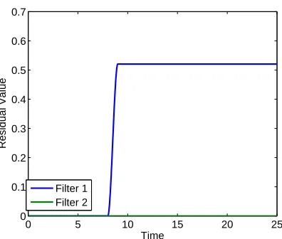
fi. If allr filters are to be created to identify allr faults, the proposition can be extended easily by requiring the hypothesis to hold for every i.

An analogous but alternative filter is given by

Proposition 3.3.2. Suppose{f1(t), . . . , fr(t)}are faults andW vli ∈/ span{W v11, W v21, W v31,

. . . ,W vd1i,W vd2i,W vd3i, . . . , W v3r}, for at least one l, where the use of d denotes missing elements. Define

MT i =

W v11, W v21, W v31, . . . W vd₁_i, W vd₂_i, W vd₃_i, . . . W v₁_r, W v₂_r, W v₃_r

,

svd(Mi) = UΣVT, and let RiT be the last columns of VT corresponding to N(Mi). Then, the following are true:

1. RiW fi(t)6= 0,∀t such thatfi(t)6= 0

2. RiW fj(t) = 0,∀t, j 6=i.

Proof. Consider RiW fj(t) = κRi g(t)W v1j+g 0₍_t₎_{W v}

2j+g

00₍_t₎_{W v}

3j

. By construction

MiRTi = 0, implying h

RiW v1j RiW v2j RiW v3j

i

= 0, for j 6= i. Therefore, the second

(37)

A more ambitious filter may sometimes be constructed. We rewrite (3.7a) and (3.7c) " r1 r2 # = " H −G # e+ " fs

−G˜f¯p # . (3.18) If " H −G #

does not have full row rank, then there exists a nontrivialR such that R

"

H

−G

#

= 0.

This leads us to

Proposition 3.3.3. Let Q= "

H

−G

#

. Suppose {f1(t), . . . , fr(t)} are faults and

W vli ∈/span{W v11, W v21, W v31, . . . ,W vd1i,W vd2i,W vd3i, . . . , W v3r, Q

T_}_,

for at least one l, where the use of _d denotes missing elements. Define

M_iT =W v11, W v21, W v31, . . . W vd1i, W vd2i, W vd3i, . . . W v1r, W v2r, W v3r, Q

,

svd(Mi) = UΣVT, and let RiT be the last columns of VT corresponding to N(Mi). Then, the

following are true:

1. RiW fi(t)6= 0,∀t such thatfi(t)6= 0

2. RiW fj(t) = 0,∀t, j 6=i

3. RiQ= 0.

Proof. Consider RiW fj(t) = κRi g(t)W v1j+g 0₍_t₎_{W v}

2j.+g

00₍_t₎_{W v}

3j

. By construction

MiRTi = 0. Hence, RiMiT = 0, implying h

RiW v1j RiW v2j RiW v3j RiQ

i

= 0, for j 6= i. The second and third statements now follow easily. The hypothesis of the proposition implies

there exists an lsuch that RiW vli 6= 0, so statement one holds.

Implementing Prop. 3.3.3 will result in

Rirj =         

0 ifi6=j

Ri 



fs

−G˜f¯p 

 ifi=j,

(3.19)

suggesting that faults can be identified immediately upon detection. As stated after Proposition

3.3.1, the hypotheses of Props. 3.3.1-3.3.3 are what are needed to create filters for faultfi. The

(38)

the hypotheses hold for all i. The filters Ri can be used in real time for identification. One

possibility of their use is given in the numerical examples in Section 3.6.

W0 and its Affect on FDI

The hypotheses on the identification theorems imply that the null spaceN(W) and rangeR(W)

of W or W0 are very important in determining which faults can be identified. N(W) denotes

a matrix whose columns are a basis for the null space. In terms of detection, (3.10) indicates that if a fault f ∈ N(W), then the fault cannot be detected. Therefore, an investigation into

the null space of W or W0 is relevant and helpful. This section studies W0 exclusively so the results in this section are applicable to fully developed (t > t1) faults only.

Proposition 3.3.4 fully characterizes the null space of W0. The proposition indicates that

the dimension of the null space is n. Recall, the fault in its constant regime is of dimension

n+m, wherenis the dimension of the state andm is the number of rows ofH. Hence, we may identify up to m distinct faults that meet the hypotheses of Props. 3.3.1-3.3.3. That is to say,

the maximum number of faults that can be identified cannot exceed the number of independent measurements.

Proposition 3.3.4. N(W0) =R "

In

HAˆ−1_G_ˆ 0

#!

.

Proof. We will need the following:

LH( Â−LH)−1+I = Â( Â−LH)−1. (3.20) The matrixLhas full column rank so multiplying the top block row ofW0 byLleaves the null

space unaffected. Then, we use (3.20) to get

˜

W0= 



−LHAˆ−LH−1Gˆ0 Aˆ

ˆ

A−LH−1L GAˆ−LH−1Gˆ0−G˜0 −G

ˆ

A−LH−1L



.

Since ˆA−1 _{exists, we can carry out the block row operation,} _G_A_ˆ−1_R

1+R2 →R2 yielding

¯

W0 = 



−LHAˆ−LH−1Gˆ0 Aˆ

ˆ

A−LH−1L GAˆ−1_G_ˆ

0−G˜0 0



.

Lemma 2.4.3 says that the (2,1) entry of ¯W0 is 0. Consider ¯W0φ= 0 and partition φ= "

φ1

φ2 #

(39)

LH)−1Lφ2 = 0. Solving forφ2 we see that

φ2 =L†( Â−LH) Â−1LH( Â−LH)−1Gˆ0φ1 (3.21a) =L†( Â−LH) Â−1(−I+ Â( Â−LH)−1) ˆG0φ1 (3.21b)

=L†LHAˆ−1Gˆ0φ1 (3.21c)

φ2 =HAˆ−1Gˆ0φ1 (3.21d)

with the restriction (I−LL†)LH( ˆA−LH) ˆG0φ1 = 0. However, this simplifies to 0φ1 = 0, so the only restriction on the null space is (3.21d).

Therefore, some of the rows of W0 are redundant. However, there are still advantages to

using both residuals, even in this constant fault case. For detection, it is clear from (3.14) that

a fault may be easier to see in certain components if we consider all rows of W0. The same is true for fault identification.

Suppose we are only concerned with process faults. This means that φ2 = 0 and we can

write a further truncated version ofW,

ˆ

W0 = "

−H( ˆA−LH)−1_Gˆ₀

G( ˆA−LH)−1Gˆ0−G˜0 #

.

Then (3.21d) implies that N( ˆW0) = N(HAˆ−1Gˆ0). The dimension of this space is important for the task of fault identification. A smaller null space will give us greater freedom to identify

faults. With this in mind, we have

Proposition 3.3.5. dim(N(HAˆ−1_Gˆ₀_{)) =}_n₋_rank(_H_). Proof. Aˆ−1 _{and ˆ}_G

0(see Lemma 2.4.4) have full column rank so rank(HAˆ−1Gˆ0) = rank(H).

Linear Combinations of Faults

As in previous sections, we are interested in a library of faults {f1(t), . . . , fr(t)}. However, in this section,fi(t) =g(t)v1i+g

0₍_t₎_v

2i+g 00₍_t₎_v

3i.fiis not scaled byκbecause here we form a fault

that is a linear combination of the fi. The scalars involved in the linear combination are our

κi values. Then we denote the faultF =Y κ, whereY = [f1. . . fj] andκ= [κ1. . . κj]T. Recall, a fault is detected if |[W Y κ]_i+ [Qh(t)]_i|> τi. Using the bound on h(t), a fault is detected if

|[W Y κ]_i|> τi+kQk(βe−α(t−t0)+).

For identification purposes we are interested in determining which faults make up the linear combination, Y, and their respective sizes κ. Creating the filters Ri according to propositions

(40)

We can also estimate κi for eachfi. Due to the construction ofRi,RiW F =κiRiW fi. This

implies |κi|kRiW fik=kRir−RiQh(t)kand noting that

kRir−RiQh(t)k ≤ kRirk+kRiQh(t)k

≤ kRirk+kRiQkθ(t)

kRir−RiQh(t)k ≥ kRirk − kRiQh(t)kr

≥ kRirk − kRiQkθ(t)

we see that

kRirk − kRiQkθ(t)

kRiW fik

≤ |κi| ≤

kRirk+kRiQkθ(t)

kRiW fik

(3.23)

assuming that the noise h(t) is small enough so thatkRirk − kRiQk(βe−α(t−t0)+)>0. The bounds on|κi|are converging at the same rate of the observer to the true value ofκi ±

kRiQk kRiW fik.

Note, this method of estimating κ is also applicable in the case where there is only one fault that is scaled by κ, not just linear combinations of two or more faults.

3.4 Disturbance Attenuation

Normal plant uncertainties are a major issue that must be addressed during FDI. Disturbances can cause false alarms, failed fault detection, and hinder fault identification. One popular

ap-proach for ODE and DAE FDI is sliding mode control [47]. Other apap-proaches include the

use of Laplace transformations to compute transfer function matrices [69] and unknown in-put observers [26]. Generally, these approaches require the disturbance to affect the differential

equation in a manner that is linearly independent to the fault in some sense. To clarify, consider the following LTI DAE with disturbance d(t) and faultsfp and fs

Ex0 =−F x+Bu+Dffp+Ddd (3.24a)

y =Hx+Du+fs. (3.24b)

One necessary assumption to decouple the disturbance using the above approaches is the rank criteria, rank [Df Dd] > max{rank(Df), rank(Dd)}. This condition may be too restrictive in

some cases. Therefore, in this section we aim to develop methods even if this condition is not

met.

Instead, we assume that the disturbances occur in a frequency bandwidth that can be

isolated from the frequencies of the faults. The faults under consideration in this paper have low