University of Windsor University of Windsor
Scholarship at UWindsor
Scholarship at UWindsor
Electronic Theses and Dissertations Theses, Dissertations, and Major Papers
8-2013
Three-Dimensional Knapsack Problem with Pre-Placed Boxes and
Three-Dimensional Knapsack Problem with Pre-Placed Boxes and
Vertical Stability
Vertical Stability
Hanan Mostaghimi Ghomi University of Windsor
Follow this and additional works at: https://scholar.uwindsor.ca/etd Part of the Engineering Commons
Recommended Citation Recommended Citation
Mostaghimi Ghomi, Hanan, "Three-Dimensional Knapsack Problem with Pre-Placed Boxes and Vertical Stability" (2013). Electronic Theses and Dissertations. 4987.
https://scholar.uwindsor.ca/etd/4987
This online database contains the full-text of PhD dissertations and Masters’ theses of University of Windsor students from 1954 forward. These documents are made available for personal study and research purposes only, in accordance with the Canadian Copyright Act and the Creative Commons license—CC BY-NC-ND (Attribution, Non-Commercial, No Derivative Works). Under this license, works must always be attributed to the copyright holder (original author), cannot be used for any commercial purposes, and may not be altered. Any other use would require the permission of the copyright holder. Students may inquire about withdrawing their dissertation and/or thesis from this database. For additional inquiries, please contact the repository administrator via email
Three-Dimensional Knapsack Problem with
Pre-Placed Boxes and Vertical Stability
By
Hanan Mostaghimi Ghomi
A Thesis
Submitted to the Faculty of Graduate Studies through Industrial and Manufacturing Systems Engineering
in Partial Fulfillment of the Requirements for the Degree of Master of Science
at the University of Windsor
Windsor, Ontario, Canada
2013
Three-Dimensional Knapsack Problem with Pre-Placed Boxes and Vertical Stability
by
Hanan Mostaghimi Ghomi
APPROVED BY:
______________________________________________ Dr. I. Ahmad
Computer Science School
______________________________________________ Dr. R. Lashkari
Industrial & Manufacturing Systems Engineering
______________________________________________ Dr. W. Abdul-Kader, Advisor
Industrial & Manufacturing Systems Engineering
DECLARATION OF ORIGINALITY
I hereby certify that I am the sole author of this thesis and that no part of this thesis has been published or submitted for publication.
I certify that, to the best of my knowledge, my thesis does not infringe upon anyone’s copyright nor violate any proprietary rights and that any ideas, techniques, quotations, or any other material from the work of other people included in my thesis, published or otherwise, are fully acknowledged in accordance with the standard referencing practices. Furthermore, to the extent that I have included copyrighted material that surpasses the bounds of fair dealing within the meaning of the Canada Copyright Act, I certify that I have obtained a written permission from the copyright owner(s) to include such material(s) in my thesis and have included copies of such copyright clearances to my appendix.
ABSTRACT
A three-dimensional knapsack problem packs a subset of rectangular boxes
inside a bin with fixed size such that the total value of packed boxes is
maximized. Each box has its own value and size and can be freely rotated into
any of the six positions while its edges are parallel to the bin’s edges. A Mixed
Integer Linear Programming is developed for the 3D knapsack problem, while
some practical constraints such as vertical stability are considered. However,
the given model can be applied to two dimensional problems as well. The
proposed solution methodology is based on the sequence triple. Simulated
annealing technique is used to model the heuristic approach. Moreover, the
situation where some boxes are placed in the bin is investigated. These
pre-placed boxes represent potential obstacles. Numerical experiments are
conducted for bins with and without obstacles. The results show that the
DEDICATION
I dedicated this thesis
To my beloved parents,
ACKNOWLEDGEMENTS
I would like to express my deepest appreciation to all those who provided me
the possibility to complete this thesis. I am thankful to my supervisor, Dr. W.
Abdul-Kader, whose advice and knowledge added to my graduate experience.
His insight has inspired me, and I would appreciate his support.
I would like to appreciate the outside reader, Dr. Imran Ahmad, for his great
advice. I am grateful to Dr. R. Lashkari for his helpful suggestions which
improved the quality of my thesis. I would also like to appreciate Dr. J. Urbanic
for chairing the thesis defence.
Furthermore, a special thanks goes to my dear friend, Omid Beiraghi, who
kindly corrected my writing. I am especially grateful to my beloved parents
TABLE OF CONTENTS
DECLARATION OF ORIGINALITY ... iii
ABSTRACT ... iv
DEDICATION ...v
ACKNOWLEDGEMENTS ... vi
LIST OF TABLES ...x
LIST OF FIGURES ... xii
LIST OF APPENDICES ... xii
LIST OF ABBREVIATIONS/SYMBOLS ... xiii
CHAPTER 1 INTRODUCTION ...1
1.1 Background ... 1
1.2 Knapsack problem ... 2
1.3 Simulated Annealing ... 5
CHAPTER 2 LITERATURE REVIEW ...8
2.1 Two-Dimensional Knapsack Problems ... 8
2.2 Three-Dimensional Knapsack Problems ... 10
2.3Research Gaps ... 16
CHAPTER 3 PROBLEM FORMULATION ...17
3.1 Problem Definition... 17
3.2 Mathematical Formulation ... 18
3.2.2 Assumptions ... 21
3.2.3 MILP ... 21
3.3 Two-Dimensional Model ... 25
CHAPTER 4 SOLUTION METHODOLOGY ...27
4.1 Three-Dimensional Algorithm ... 27
4.1.1 Sequence Triple ... 27
4.1.2 Placement Algorithm ... 28
4.1.3 Simulated Anealing ... 30
4.1.4 Orthogonal Rotation ... 32
4.1.5 Obstacles ... 32
4.1.6 Four Corners Packing ... 33
4.1.7 Order of Box Insertion ... 33
4.2. Two-Dimensional Algorithm ... 33
CHAPTER 5 NUMERICAL ANALYSIS ...35
5.1 Intoduction ... 35
5.2 Numerical Experiments ... 35
5.3 Parameter Setting ... 38
5.4 Results and Sensitivity Analysis ... 38
5.5 Algorithm Verification ... 47
5.6 Conclusion ... 48
CHAPTER 6 CONCLUSIONS AND FUTURE WORKS ...49
6.1 Conclusions ... 49
6.2 Future Works ... 50
REFERENCES/BIBLIOGRAPHY...51
APPENDICES ...54
Appendix A ... 54
Appendix C ... 67
LIST OF TABLES
Table 2.1: Summary of Some Relevant Papers ...14
Table 3.1: 2D Rectangles Dimensions and Maximum allowed Number...26
Table 5.1: Information on the First Set of Boxes ...36
Table 5.2: Information on the Second Set of Boxes ...36
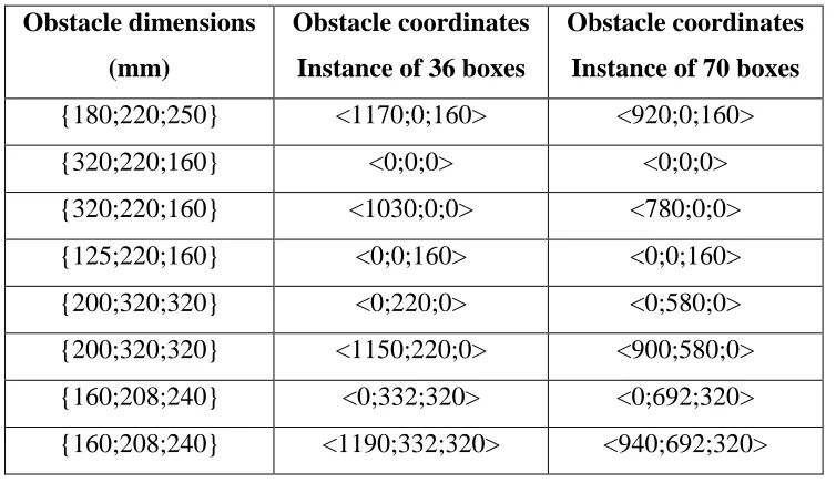
Table 5.3: Obstacles Dimensions and Coordinates for Instances with 36 and 70 Boxes ...37
Table 5.4: Ceiling and Middle Obstacles Information ...37
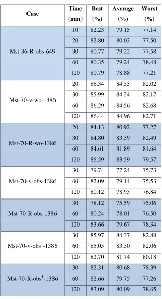
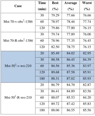
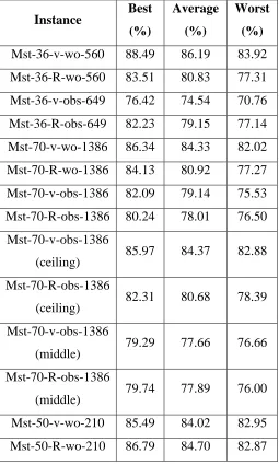
Table 5.5: Worst, Best, and Average Utilization ...38
LIST OF FIGURES
Figure 1.1: Knapsack Problem Types ...3
Figure 1.2: Simulated Annealing Block Didgram ...7
Figure 3.1: The X, Y, and Z axes of the bin ...21
Figure 3.2: 2D Instance Result...26
Figure 5.1: Best Result for Mst-36-v-wo-560 ...42
Figure 5.2: Best Result for Mst-36-R-wo-560...43
Figure 5.3: Best Result for Mst-36-R-obs-649 ...43
Figure 5.4: Best Result for Mst-36-v-obs-649 ...43
Figure 5.5: Best Result for Mst-70-v-wo-1386 ...44
Figure 5.6: Best Result for Mst-70-R-wo-1386...44
Figure 5.7: Best Result for Mst-70-R-obs-1386 ...44
Figure 5.8: Best Result for Mst-70-v-obs-1386 ...45
Figure 5.9: Best Result for Mst-70-v-obs(ceiling)-1386 ...45
Figure 5.10: Best Result for Mst-70-R-obs(ceiling)-1386 ...45
Figure 5.11: Best Result for Mst-70-v-obs(middle)-1386 ...46
Figure 5.12: Best Result for Mst-70-R-obs(middle)-1386 ...46
Figure 5.13: Best Result for Mst-50-v-wo-210 ...46
Figure 5.14: Best Result for Mst-50-R-wo-210...47
LIST OF APPENDICES
Appendix A: Number of packed boxes of each type in some of the best
obtained results ...54
Appendix B: Packed boxes coordinates for some of the best results ...56
LIST OF ABBREVIATIONS/SYMBOLS
C&P Cutting and Packing
MILP Mixed Integer Linear Programming
3D Three-Dimensional
2D Two-Dimensional
CHAPTER 1
Introduction
1.1.Background
Cutting and packing problems have been intensely studied as they have many
applications in industrial and finance management. The three dimensional packing
problem is essential for practical purposes such as container loading or scheduling
which can be defined as a geometric assignment problem. The various packing
problems can have different constraints and objectives. For instance, in the case of
shipping, objects with different sizes have to be packed into a larger container. A
topology of packing problems in general was defined by Dyckhoff et al. (1990) and a
recent survey was defined by Wascher et al. (2007). Cutting and packing problems
appear under several different names such as bin packing, multi-container loading
problem, strip packing and knapsack problems, based on the objective function and
the side constraints. All types of cutting and packing problems have some similar
structures. They consist of two sets of elements, a set of large objects (called bins) and
a set of small items (called boxes). The problem is to select some or all small items
and assign them to one of the large objects while all selected small items are placed
entirely in the large object and do not overlap and a given objective function is
optimized. Thus, only some of the large objects and small items may be used in a
solution of the problem. The packing problem considers optimal utilization of bin
volume for goods distribution and is an important industrial problem. Filling a bin
optimally decreases the shipping cost and increases the stability of the load. The large
objects, which are called bins, can be homogeneous or heterogeneous. If the boxes
placed in the given bin are identical it is called homogeneous; however, if various
types of boxes are placed in it, it is considered as strongly heterogeneous.
Different kinds of cutting and packing problems can be divided to two categories.
In the first category, sufficient bins are available to pack all the boxes; however, only
a limited number of bins is available to pack a subset of boxes in the second category.
The first type of problems are called an input minimization problem, and the second
type are called an output maximization type. In the case of output maximization, a set
However, in the case of input minimization, all the boxes can be packed. In strip
packing problem, a set of rectangular boxes are packed in a strip with certain width
and height and variable length. The problem is how to place all the boxes inside the
strip such that its length is minimized. In bin-packing problem, a set of items have to
be packed in a set of bins of the same fixed sizes and costs, such that the number of
used bins is minimized. Unlike bin-packing problem, in multi-container loading
problem, the containers (or bins) do not essentially have equal sizes and costs. In
knapsack problem each item has a profit and the problem is to choose the best subset
of items that fits into the single bin or container such that the sum of the items profit is
maximized. In this kind of problem, the availability of bins is limited so all items
cannot be packed. (Leung, 2012; Fekete & Schepers 1997; Wei et al. 2009; Egeblad et
al. 2010; Pisinger 2002).
1.2. Knapsack Problem
The knapsack problem is a problem in combinatorial optimization. The
multidimensional knapsack Problem (MKP) is a strongly NP-hard optimization
problem which can be show by reduction from the one-dimensional packing problem;
it means that it is very unlikely to develop polynomial algorithms for these problems.
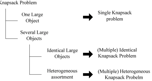
Knapsack problems consist of three different types. The first one is Single Knapsack
Problem (SKP), the problem of packing a subset of strongly heterogeneous boxes in a
single container. Multiple Identical Knapsack Problem is the second type which
considers packing a subset of strongly heterogeneous boxes in a set of identical bins.
The last type is Multiple Heterogeneous Knapsack Problem (MHKP) which is the
problem of packing a subset of strongly heterogeneous boxes in a set of weakly and
strongly heterogeneous bins. Figure 1.1 shows the different types of knapsack
Figure 1.1 Knapsack Problem Types, Wascher et al. (2007)
Various practical constraints can be considered in the multidimensional knapsack
problems. Some of these constraints are related to the bin, while some of them may
refer to the boxes. Moreover, some constraints might be related to the relationship
between the bin and boxes. One such constraint is the orientation constraint.
Principally, each box dimension can be considered as height, thus three other
orientations can easily be defined. Each box can have six orientations in order to
orthogonally be placed in a bin. Moreover, one other practical constraint is the
positioning constraint which limits the location of the boxes in the bin.
Load stability constraint is one of the most important issues in knapsack problems.
In spite of its importance, load stability is often not studied explicitly in the literature.
The stability is a direct consequence of load trimness when high bin utilization can be
assured. This is typically true for knapsack problems in which only a subset of boxes
can be packed as the bin availability is limited. Load stability can be divided into
vertical and horizontal stability. Vertical stability prevents boxes from falling down
onto bin floor or on top of other boxes. It deals with gravity force. In order to satisfy
this kind of stability, the bottom of a box should be supported by the bin floor or other
box tops. Horizontal stability or dynamic stability guarantees that boxes cannot shift
notably when the bin is moving. Horizontal stability is satisfied when each packed
box is adjacent to other boxes or to the bin wall.
In addition, another constraint which can be considered in knapsack problems is
by a series of cuts which are in parallel to the bin walls. Guillotineable patterns are
not always suitable for packing as the boxes tend to be more unstable while being
transported. A robot packable packing is one which can be done by placing boxes
starting from left-bottom-behind corner of a bin, while each box is placed in front, on
the right or above the already packed boxes. Robot packable packing tackles a
situation in which a robot with artificial hands packs the boxes into the bin.
Although technological knowledge has enhanced, solving real knapsack problems
is still a challenge. The solution quality and computational efficiency are very
sensitive to the box-positioning rule. Due to NP-hardness of the packing problem,
only few exact algorithms and many heuristic methods have been presented which are
based on the different strategies (Leung, 2012; Fekete & Schepers, 1997; Wei et al.,
2009; Egeblad et al., 2010; Pisinger, 2002; Bortfeldt & Wascher, 2012).
The problem addressed here, in the topology suggested by Dyckhoff (1990),
belongs to 3/B/O/F (3: three-dimensional, B/O: one object/bin and items selection, F:
few items of different types) while Wascher et al. (2007) classify it as the
three-dimensional single orthogonal knapsack problem. As well as non-overlapping
constraints, some other constraints should be considered in practice, such as bin
stability and pre-placed boxes. The given problem considers the packing of
rectangular items in a rectangular bin in order to maximize the total value of the
packed items (minimize the amount of space loss).The value of boxes is assumed to
be equal to their volume. The rotation of the boxes is taken into account as well. Since
the three-dimensional knapsack problem is NP-hard, it is difficult to solve. In
addition, the difficulty of finding optimal solution is enhanced as the box rotations
increase the search space significantly. Some exact algorithms as well as heuristic
methods are proposed in the published literature. Since exact algorithms need more
time to find a solution, heuristic approaches are more popular and can be used as an
alternative to find near optimal solutions. A mixed integer linear model is developed
for the given knapsack problem. The model considers vertical stability and pre-placed
constraints which were not studied in Egeblad and Pisinger (2009). These practical
constraints as well as the box rotations are added to the model in order to study a
realistic knapsack problem. The proposed three-dimensional solution methodology is
The developed algorithm also considers box rotation, pre-placed boxes and vertical
stability. Simulated annealing is used as a heuristic method.
1.3. Simulated Annealing
Simulated annealing (SA) is a general optimization method to solve combinatorial
optimization problems. It belongs to the class of local search algorithms. Simulated
annealing algorithm has been used to handle many NP-hard problems. It was
developed in 1983 to solve nonlinear problems. The inspiration comes from annealing
in metallurgy, a technique of heating and controlled cooling of material in order to
enhance the size of its crystal and decrease their defects, so that its structure is finally
frozen which occurs at a minimum energy configuration. Simulated annealing
algorithm is based on the very important fact that even in low temperature it is
probable to have a particle with high internal energy. This fact shows the possibility
of jumping out of the local minimum. While the temperature is reduced, the
possibility of jumping out decreases. The basic elements of simulated annealing are as
follows:
1. A finite set S.
2. A cost function which is defined on S.
3. A set S(i)⊂S −{i}∀i∈S which is the set of the neighbours of i.
4. Cooling schedule T which is a non-increasing function. T(t) is the temperature
at time t.
5. An initial state.
The slow cooling is applied to the simulated annealing method as a slow reduction
in the probability of accepting worse solutions. At each step, the algorithm considers
some neighbouring states of the current state, and decides whether to stay at the
current state or move to a neighbouring state. The probability of moving from a
current state to a new neighbouring state is called acceptance probability which
depends on the energies of the two states and a control parameter known as
temperature. If the energy of the new state is better than the current one, the
worse, the move to the new state is accepted if
e
(−∆temperature)>R , whereenergy state
current
energy state
new energy state
current
_ _
) _
_ _
_
( −
=
∆ , and R=Uniform(0,1). At first, T
has a relatively high value, so the chance to accept the new state is higher. T is slowly
decreased to values such that most new states will not be accepted. The algorithm is
repeated until it achieves a state that is good enough for the given application or until
a given computation time is exhausted. It has been proved that by controlling cooling
rate of temperature this algorithm can find the global optimum, although it needs
infinite time. Like all other algorithms, simulated annealing has some strengths and
weaknesses. It can deal with chaotic data, highly nonlinear problems and many
constraints. It is able to reach global optimality. Simulated annealing algorithm is
relatively flexible as it does not depend on any restrictive model’s properties.
However, as SA is a metaheuristic algorithm, so many choices are required to
consider in the actual algorithm. Obviously, there is a trade-off between the quality of
the solutions and computation time. Figure 1.1 shows the block diagram of simulated
CHAPTER 2
Literature Review
2.1. Two Dimensional Knapsack Problem
Some papers in this area focus on two-dimensional packing problem. Leung et al.
(2001) present a genetic algorithm and a simulated annealing approach to solve the
two-dimensional non-guillotine cutting stock problem. They aim to find a cutting
pattern which minimizes trim loss. The authors apply the genetic algorithm and
simulated annealing to determine the permutations of small trim loss; then they use
different packing approaches to pack the items corresponding to a special
permutation. The proposed heuristic cannot produce all the feasible packings.
Capara and Monaci (2004) consider upper bounds and exact algorithm for the
two-dimensional orthogonal knapsack problem. The authors present an approximation
algorithm and four exact algorithms based on the enumeration scheme, and mainly
focus on upper bounds. They claim their algorithm has similar performance to Fekete
and Schepers’ (1997) algorithms in most instances.
Clautiaux et al. (2007) consider the two-dimensional orthogonal knapsack problem
and propose two exact methods to solve the problem. In the first algorithm, they
improve the classic branch and bound method; however, the second one is on the
basis of a new relaxation of the problem. They, moreover, define the reduction
procedures and lower bounds used within both enumerative methods. The first
algorithm is called LMAO (Leftmost Active Only) which counts the packing of items
only in the left-most-downward position and tests the possibility of not packing any
item in that position. By using this algorithm the same packing is not counted twice.
The second algorithm called Two Step Branching Procedure (TSBP) is based on
cutting each item with wi and height hi into hi strips with width wi. All strips relating
to the given item must be packed at the same coordinate even if they are not similar.
Goncalves (2007) proposes combination of the placement procedure and a genetic
algorithm based on random keys to solve a two-dimensional orthogonal knapsack
problem. The objective function is minimizing the amount of trim loss. The proposed
algorithm is relatively complex and time consuming.
Bortfeldt and Winter (2009) propose a genetic algorithm for the two dimensional
orthogonal knapsack problems. The proposed algorithm considers both guillotine and
non-guillotine variant of the problem and an orientation constraint also may be
considered. The items which have to be placed in the container can be constrained as
well as unconstrained. The authors claim that for large instances of the non-guillotine
constrained 2D knapsack, GA solution is significant.
Joncour et al. (2010) suggest a method for finding a feasible solution for a two
dimensional orthogonal knapsack problem which is based on the characterization of
the interval graph. The problem is packing the rectangular items in a big rectangular
container without overlapping. It is assumed that the rotation of the items is not
allowed. In order to find infeasible solutions earlier, they used a method similar to
Clautiaux et al. (2007). The approach suggested in this paper is superior to the Fekete
and Schepers’ (1997) method since by creating MPQ-trees, the search space stays
within the set of interval graphs.
Dolatabadi et al. (2012) propose a recursive exact algorithm to solve the
two-dimensional guillotine knapsack problem. The problem is packing small rectangular
items in a bigger rectangular sheet. The packing is orthogonal and the rotation of the
items is not allowed. At first, the sets of associated guillotine packing are built; then,
the algorithm is divided into two exact algorithms in order to solve the
two-dimensional knapsack problem. The first algorithm is on the basis of iterative
implementation of recursive method with different input parameters, and the second
one is based on an ILP model. The branch-and-cut method is used to confirm the
optimality of the solution.
Leung et al. (2012) propose a hybrid simulated annealing metaheuristic for the
two-dimensional knapsack problem. The authors first define a fitness strategy to identify
the solution based on this fitness strategy. Finally, the simulated annealing approach is
used to jump out of the greedy strategy’s local optimal trap. The items are packed into
stock sheet one at a time for a given sequence of items. For any available position, the
fitness value of each item, which has to be packed, is calculated and then the item
with maximum fitness value is selected. If more than one item has the same maximum
fitness value, the algorithm selects the one by the input order of the items. The
proposed hybrid algorithm combines the greedy strategy approach and simulated
annealing to gain a better solution. The greedy algorithm is used to search a good
sequence of items; then a simulated annealing heuristic is applied to do a broader
search to gain a better solution.
2.2. Three Dimensional Knapsack Problem
Some papers consider the three dimensional cutting and packing problem (or
container loading) and attempt to model it or propose solution methodology for such
problems. The focus of most of these papers is on the rectangular bins. As multi
dimensional C&P problems are strongly NP-hard, only very few exact algorithms
have been proposed for such problems.
Fekete and Schepers (1997) propose a method for modeling more-dimensional
packing problem based on the graph characterization of feasible packing. They define
a graph based on the relative positions of boxes. The graph is proven to be an interval
graph. The authors consider a set of boxes to be packed into a container and focus on
an orthogonal packing problem. The method cannot handle further constraints like
fixing the position of some items, and the results are limited to two dimensional
problems. Fekete and Schepers (1997) present a method in order to gain lower bounds
for more-dimensional knapsack problem. They, moreover, illustrate that all known
lower bounds for such problems can be improved by this method. The authors
describe heuristics for dismissing infeasible packings. Fekete and Schepers (1997)
show how this method can be applied to more dimensional knapsack problem.
Fekete and Schepers (2004) propose a new method for obtaining classes of lower
bound for higher-dimensional packing problem. The authors apply a number of
the way that they can be combined is reflected by transformation. They present a
combinatorial characterization of feasible packing as a basis for branch and bound
approach. The major objective of this paper is to define good criteria for removing a
candidate set of boxes. Dual feasible function is a way to build conservative scales.
All known classes of lower bound for higher-dimensional packing problem can be
improved by using the proposed approach. The authors suggest a strong method for
solving higher dimensional problems by combining these classes of bounds and
characterization of feasible packing as described in Fekete and Schepers (1997). The
computational results are mainly limited to the two-dimensional packing problem.
Hifi (2004) proposes a dynamic algorithm and an exact depth-first search in order to
solve the three dimensional cutting problem. Orientation and guillotine constraint are
considered. Sixty four problem instances were tested which include up to 50 boxes.
Optimal solutions are obtained for most of the instances but not all of them.
Although considerable advancement has been made in the development of exact
algorithms, heuristic algorithms still play an important role in solving
three-dimensional knapsack problems. Only heuristic methods can provide reasonable
solutions within acceptable running times for problem instances of real-world size.
Martello et al. (2007) consider the orthogonal three-dimensional bin packing problem
where box rotation is not allowed. Both general and robot packable variants of
bin-packing problem are presented. The algorithm is on the basis of two-level
decomposition approach and consists of two parts. In the first part the boxes are
assigned to the bins. In the second part, a single bin is filled while the objective
function is maximizing the filled volume. The proposed methodology can be used as a
whole for solving the three-dimensional bin packing problem or just for filling a
single bin.
Egeblad and Pisinger (2009) propose a simulated annealing based methodology for
the two and three dimensional knapsack problems. A three-dimensional knapsack
model is presented. New constraints can be added to this model such as fixing the
position of items or rotation. The authors present an iterative heuristic for the
the sequence pair is transformed to the packing. In order to control the heuristic
method simulated annealing is used. For three-dimensional knapsack problem,
sequence triple technique is used. The authors prove that a fully robot packable
packing can be obtained through sequence triple representation. Robot packing is a
packing obtained by locating items starting from left-bottom-behind (LBB) corner. It
is represented in three sequences; for any sequence the relationship of each two items
is defined. To find a placement for any given sequence, three constraint graphs are
constructed. Like 2DKP, the meta-heuristic annealing is used to solve the
dimensional knapsack problem. Rotation of boxes is not considered in the
three-dimensional model and experiments.
Wu et al. (2010) consider the three-dimensional bin packing problem with variable
bin height. The bins and boxes are rectangular and the object rotation is allowed.
Guillotine constraint is not imposed. Moreover, bin heights can change in order to fit
bin contents. A mixed integer programming model is proposed, and a bin packing
algorithm which is based on packing index is used to develop the problem feature and
as a building block for genetic algorithm. The authors also present the situation when
more than one type of bin is used. A genetic algorithm-based heuristic is proposed for
packing a batch of objects. The algorithm is on the basis of extreme point method.
The authors consider both single bin packing and batch bin packing problems.
Amossen and Pisinger (2010) consider the multi-dimensional orthogonal bin-packing
problem with guillotine constraints where rotation is not allowed. The authors
experimentally evaluate three packing methods –unrestricted, robot packable,
guillotine cuttable- based on the solution time and quality.
Models provide information on optimal objective function value and bounds. They are
helpful to assess the solution quality of heuristic algorithms. Modeling three
dimensional knapsack problems, while considering practical constraints, is still at its
beginning.
Junqueira et al. (2012) present mixed integer linear programming models for the
container loading problem. Vertical and horizontal stability of the cargo as well as
can be extended in order to apply to other variants of container loading problem as
well. However, the models are only able to handle moderate size problems.
In addition, container loading problems have been studied from a more general and
practical view. Murty et al. (2005) propose a decision support system in order to
develop optimal decisions. These decisions are used to route container trucks, find the
storage place for containers, number of assigned container and truck scheduling. The
proposed decision system is applied to the Hong Kong International Terminals. Murty
et al. (2005) define a selection of inter-related decisions which is made at the
container terminal during a day. The main goal of these decisions is minimizing the
resource and the trucks waiting time, and maximizing the container volume
utilization. The author use decision support systems to make these decisions since
these kinds of decisions are complex and large scale. Petering and Murty (2009)
develop a simulation study about terminal’s average quay crane rate, and how the
long-run performance of seaport container terminal is related to storage block length
and yard crane deployment. Several scenarios are evaluated. These experiments are
direct connection between length of the block and long-run performance in the
container terminal.
As mentioned, both exact algorithms and heuristic methods are proposed in the
published literature. Leung et al. (2001), Goncalves (2007), Bortfeldt & Winter
(2009), Leung et al. (2012), Egeblad & Pisinger (2009) and Wu et al. (2010) propose
heuristic algorithms for different types of packing problems. While, Fekete &
Schepers (1997), and Hifi (2004) propose exact methods. The following table
compares some relevant papers and models, and shows their similarities, differences
Table 2.1. Summary of Some relevant Papers
Papers Problem type Assumption What they do? Solution
Methodology
Superiority to other
papers Limitation
Egeblad & Pisinger (2009)
2D and 3D knapsack problem
Items are strongly heterogeneous, no rotation Mathematical Model sequence based representation (SA based approach)
Sequence pair and triple is one of the successful representations
Fixed orientation for 3D Bortfeldt & Winter (2009) 2D Orthogonal knapsack problem
Guillotine & non-guillotine, orientation constraint may be considered
Heuristic algorithm GA
GA is suitable for large instances of the non-guillotine constrained
compare to other methods GA is in the mid-table Junqueira et al.
(2012)
container loading problem
vertical and horizontal stability, load bearing strength
MILP GAMS
extend in other variants of container loading problem
Only able to handle moderate size problems
Wu et al. (2010)
3D bin packing problem with variable bin height
Rectangular boxes, , Guillotine constraint is not imposed
Mathematical Model GA & extreme point
both single bin packing and batch bin packing problem is considered, object rotation is allowed Amossen & Pisinger (2010) multi-dimensional orthogonal bin-packing problem Guillotine, no rotation
evaluate three packing methods
unrestricted, robot packable, guillotine cuttable
Fixed orientation
Martello et al. (2007)
3D orthogonal bin packing problem
rotation is not allowed, general and robot packable Decomposition algorithm two-level decomposition approach
can be used as a whole for solving three-dimensional bin packing problem or just for filling a single bin
Fixed orientation Goncalves (2007) 2D knapsack problem Orthogonal, fixed orientation
Solving 2D packing problem
Hybrid genetic algorithm
Relatively complex, long computational time compared to Leung et al. (2012) Leung et al.
(2001)
2D non-guillotine cutting stock
Fixed orientation,
orthogonal, Heuristic algorithm
Genetic algorithm and simulated annealing
Fekete & Schepers (1997)
More-dimensional packing problem
Fixed orientation, orthogonal
Modeling packing based on the graph characterization of feasible packing
Interval Graph
method cannot handle further constraints
Given Problem 3D knapsack
problem Rectangular boxes
Finding more practical packing, Mathematical formulation
SA and sequence triple
2.3. Research Gaps
According to the literature, not all papers consider box rotation since it increases the
search space significantly. Moreover, bin stability is just taken into account in some
of the container loading problems and it has not been considered in three-dimensional
knapsack problem. Vertical stability is one of the realistic constraints which should be
taken into account in 3D knapsack problems, so all the packed boxes are supported by
the bin floor or other boxes top and do not fall down. In addition, to the best of our
knowledge, pre-placed boxes (obstacles) has not been studied in three-dimensional
knapsack problems, which is so essential for such problems since it is often required
to place certain boxes in certain positions. Such a constraint can be also considered
when the bin does not have rectangular shape. Therefore, it is important to study more
practical constraints in the knapsack problem. In the given problem, box rotation is
taken into account in order to find more practical packings. Also, preplaced boxes
(bin with some obstacles) and vertical stability which are real-world constraints are
CHAPTER 3
Problem Formulation
3.1. Problem Definition
In this study, the three-dimensional knapsack problem is considered where there is
one bin with fixed size and a set of boxes; each box has an associated size. The aim is
to find an efficient solution methodology in order to pack rectangular boxes in a
single bin so that the total value of the packed boxes is maximized, or equivalently the
empty spaces left are minimized. The boxes are assumed to be strongly heterogeneous
which means there is a relatively high number of different types of boxes and a small
number of boxes for each box type (Wascher et al., 2007). Moreover, the packing is
considered feasible if each box lies entirely in the bin, and the packed boxes do not
overlap. The edges of all boxes must be parallel to the edges of the bin (orthogonal
packing). The bin and boxes are assumed to be of rectangular shape.
Some practical considerations which play an important role in modeling more realistic
knapsack problems are presented such as box rotation and bin stability. Boxes are able
to freely rotate in six different orientations, need not to be packed in layers, and the
bottom of each box must be supported by the top of other boxes or the bin floor. In
addition, some boxes are considered as pre-placed boxes or obstacles, whose
left-bottom-behind (LBB) corner should be placed in a specific position. The value of
each box is equal to its volume. It is assumed that the dimensions of all boxes and the
bin are integers, thus the placement are to be done in integer steps. Let C be a
rectangular container with width W, height H and depth D. The origin of the Cartesian
coordinate system is located at the LBB corner of the container, and li, hi, and wi are
respectively, the length, height and depth of box type i. For each packed box, (xi, yi,
zi) represents the coordinates of the LBB corner of the box.
A mixed integer programming formulation is presented for the given problem. Some
real-world knapsack problem constraints are considered in the model which, to the
best of our knowledge, have not been studied yet. These constraints are vertical
stability and pre-placed boxes. Since the three-dimensional knapsack problem is
significantly increases the search space, so the difficulty of finding the optimal
solution is enhanced as well. Some exact algorithms as well as heuristic methods are
proposed in the published literature. As exact algorithms require more time to find a
solution, heuristic approaches are more popular and can be good alternatives to find
optimal or near optimal solution. The proposed three-dimensional solution
methodology is based on Egeblad and Pisinger’s (2009) sequence triple
representation. Simulated annealing is used as heuristic method.
3.2. Mathematical Formulation
A mixed-integer programming model of the 3D-knapsack problem is introduced in
this section. The mathematical model is based on Egeblad and Pisinger (2009) and
Wu et al. (2010). Some modifications are made in their model which include
considering vertical stability and pre-placed boxes constraints. Egeblad and Pisinger
(2009) and Wu et al. (2010) do not consider these important and practical constraints.
Constraints (1) – (4) are based on Egeblad and Pisinger (2009); they did not consider
the box orientation in their model. The binary position variables which show the
orientation of the boxes are based on Wu et al. (2010). However, constraints (5) – (17)
are new constraints added to the model which are described in the following sections.
3.2.1. Notations
The variables and parameters used in the mathematical formulation are introduced as
follows:
• Variables:
(xi,yi,zi): LBB coordinates of box i
Xwi, Zwi: 1 whether width of box i is parallel to the container’s X and Z
0 otherwise
Yhi: 1 if height of box i is parallel to the container’s Y
Zdi: 1 if depth of box i is parallel to the container’s Z
0 otherwise
rij, lij: 1 if box i is to the right of or to left of box j
0 otherwise
oij, uij: 1 if box i is over or under box j
0 otherwise
bij, fij: 1 if box i is behind or in-front-of box j
0 otherwise
si: 1 if box i is packed
0 otherwise
yaij: 1 if xj≥ xi
0 otherwise
xaij: 1 if xj < x’i
0 otherwise
ybij: 1 if zj≥ zi
0 otherwise
xbij: 1 if zj < z’i
0 otherwise
ycij: 1 if x’j > xi
0 otherwise
xcij: 1 if x’j ≤ x’i
ydij: 1 if z’j > zi
0 otherwise
xdij: 1 if z’j ≤ z’i
0 otherwise
zaij: 1 if xi≤ xj < x’i
0 otherwise
zbij: 1 if zi≤ zj < z’i
0 otherwise
zcij: 1 if xi < x’j≤ x’i
0 otherwise
zdij: 1 if zi < z’j≤ z’i
0 otherwise
Cs1: 1 if xi≤ xj < x’i and zi≤ zj < z’i
0 otherwise
Cs2: 1 if xi≤ xj < x’i and zi < z’j≤ z’i
0 otherwise
Cs3: 1 if xi < x’j≤ x’i and zi≤ zj < z’i
0 otherwise
Cs4: 1 if xi < x’j≤ x’i and zi≤ zj < z’i
0 otherwise
x’i = xi + wiXwi + hi(Zwi – Yhi + Zdi) + di(1 - Xwi – Zwi + Yhi – Zdi)
• Parameters:
(wi,hi,di): width, height and depth of box i
(W,H,D): width, height and depth of the container
(r,s,k): LBB coordinates of the pre-placed boxes
(a, b, c, d): Binary orientation parameters of the pre-placed boxes
Pi: value of box i
3.2.2. Assumptions
The following assumptions are considered for the mix integer linear model:
1. The boxes are strongly heterogeneous.
2. The boxes must be located orthogonally
3. The boxes are able to freely rotate
4. The box and bin dimensions are assumed to be non-negative integer
5. The value of a boxes is equal to its volume
6. The X, Y, and Z axes of the bin are shown in the following figure.
Figure 3.1. The X, Y, and Z axes of the bin
3.2.3. MILP
The objective Function is maximizing the value of packed boxes:
∑
= n
i
i i
s
P
Max1
Subject to:
rij + lij + bij + fij + uij = si + sj -1 ∀i,j i≠j (1)
xi + wiXwi + hi(Zwi – Yhi + Zdi) + di(1 - Xwi – Zwi + Yhi – Zdi) ≤ xj + M(1-lij)
∀i,j i≠j (2a)
xj + wjXwj + hj(Zwj – Yhj + Zdj) + dj(1 – Xwj – Zwj + Yhj – Zdj) ≤ xi + M(1-rij)
∀i,j i≠j (2b)
zi + diZdi + hi (1 – Zwi – Zdi) + wiZwi≤ zj + M(1-bij) ∀i,j i≠j (2c)
zj + djZdj + hj (1 – Zwj – Zdj) + wjZwj≤ zi + M(1-fij) ∀i,j i≠j (2d)
yi + hiYhi + wi(1 – Xwi – Zwi) + di(Xwi + Zwi – Yhi) ≤ yj + M(1-uij)
∀i,j i≠j (2e) yj + hjYhj + wj(1 – Xwj – Zwj) + dj(Xwj + Zwj – Yhj) ≤ yi + M(1-oij)
∀i,j i≠j (2f) xi + wiXwi + hi(Zwi – Yhi + Zdi) + di(1 - Xwi – Zwi + Yhi – Zdi) ≤ W (3a)
yi + hiYhi + wi(1 – Xwi – Zwi) + di(Xwi + Zwi – Yhi) ≤ H (3b)
zi + diZdi + hi (1 – Zwi – Zdi) + wiZwi≤ D (3c)
Xwi + Zwi≤ 1 (4a)
Zwi + Zdi ≤ 1 (4b)
0 ≤ Zwi - Yhi + Zdi ≤ 1 (4c)
0 ≤ 1- Xwi - Zwi + Yhi - Zdi ≤ 1 (4d)
0 ≤ Xwi + Zwi - Yhi≤ 1 (4e)
(xi, yi, zi) = (r, s, k) ∀i ∈Pb (5)
xj – xi≤ M. yaij xj – xi≥ M (yaij – 1) (7a)
x’i – xj≤ M. xaij x’i – xj≥ M (xaij – 1) + 0.5 (7b)
(yaij + xaij – 1) ⁄ 2≤ zaij≤ (yaij + xaij) ⁄ 2 ∀i,j i≠j (7c)
zj – zi≤ M. ybij zj – zi≥ M (ybij – 1) (8a)
z’i – zj≤ M. xbij z’i – zj≥ M (xbij – 1) + 0.5 (8b)
(ybij + xbij – 1) ⁄ 2 ≤ zbij≤ (ybij + xbij) ⁄ 2 ∀i,j i≠j (8c)
x’j – xi≤ M. ycij x’j – xi≥ M (ycij – 1) + 0.5 (9a)
x’i – x’j≤ M. xcij x’i – x’j≥ M (xcij – 1) (9b)
(ycij + xcij – 1) ⁄ 2 ≤ zcij≤ (ycij + xcij) ⁄ 2 ∀i,j i≠j (9c)
z’j – zi≤ M. ydij z’j – zi≥ M (ydij – 1) + 0.5 (10a)
z’i – z’j≤ M. xdij z’i – z’j≥ M (xdij – 1) (10b)
(ydij + xdij – 1) ⁄ 2 ≤ zdij≤ (ydij + xdij) ⁄ 2 ∀i,j i≠j (10c)
(zaij + zbij – 1) ⁄ 2 ≤ Cs1≤ (zaij + zbij) ⁄ 2 ∀i,j i≠j (11)
(zaij + zdij – 1) ⁄ 2 ≤ Cs2≤ (zaij + zdij) ⁄ 2 ∀i,j i≠j (12)
(zcij + zbij – 1) ⁄ 2 ≤ Cs3≤ (zcij + zbij) ⁄ 2 ∀i,j i≠j (13)
(zcij + zdij – 1) ⁄ 2 ≤ Cs4≤ (zcij + zdij) ⁄ 2 ∀i,j i≠j (14)
Cs1 + Cs2 + Cs3 + Cs4 = uij + oij ∀i,j i≠j (15)
x’i = xi + wiXwi + hi(Zwi – Yhi + Zdi) + di(1 - Xwi – Zwi + Yhi – Zdi) (16)
z’i = zi + diZdi + hi (1 – Zwi – Zdi) + wiZwi (17)
rij, lij, bij, fij, uij∈ {0,1} (18)
xaij, xbij, xcij, xdij,yaij, ybij, ycij, ydij, zaij, zbij, zcij, zdij∈ {0,1} (20)
si, Cs1, Cs2, Cs3, Cs4 ∈ {0,1} (21)
(xi ,yi, zi) ≥ 0 (22)
Constraint (1) ensures that if box i and box j are packed then they must be placed left,
right, under, over, behind or in-front-of each other. Constraints (2) guarantee that any
two boxes i and j do not overlap, while considering the box rotation. It includes six
parts; constraint (2a) and (2b) find the x coordinate of the box to be packed; constraint
(2c) and (2d) are used to find its z coordinate, and constraint (2e) and (2f) calculate its
y coordinate. The binary position variables (Xwi, Zwi, Yhi, Zdi) are used to allow box
rotations. Constraint set (3) ensures that all boxes are placed within the bin’s
dimensions. Constraint (3a) makes sure that the box dimensions do not exceed the
bin’s width; while constraints (3b) and (3c) are related to the bin’s height and depth.
Constraint set (4) is used to make sure that the binary variables which show the
position of the boxes are controlled to represent practical positions. Constraint (4a)
guarantees the width of the packed box is not parallel to both X and Z axis. Constraint
(4b) ensures that the width and depth of each packed box are not parallel to Z axes
simultaneously. Constraint (4c) shows that the height of box i cannot be parallel to
both Z and Y axes. Constraints (4d) and (4e) also control the orientation of the packed
boxes, and ensure that the width, height, and depth of each packed box are not parallel
to two axes simultaneously. Constraint (5) and (6) are used to fix the coordinates and
orientation of the pre-placed boxes, where Pb is a set of preplaced boxes. Constraints
(7)–(10) ensure vertical stability. These constraints compare the four corners of each
newly packed box with the points that cover the top of other packed boxes. If one of
the corners has the same x and z coordinates as one of the mapped points, it means
that the new box is located under or above that box. Constraint set (7) is used to
define the binary variable zaij and includes three parts. Constraint (7a) ensures that if
xj ≥ xi, then yaij is equal to one; otherwise it is equal to zero. Constraint (7b) makes
sure that if xj < xi, then xaij is one; otherwise it is equal to zero. Constraint (7c)
guarantees when yaij and xaij are both equal to one, then zaij is equal to one. Similarly,
constraint sets (8), (9), and (10) are used to define the binary variables zbij, zcij, and
zdij. Constraints (11)-(14) show whether the x and z coordinates of the new box’s
boxes. Constraint (15) ensures that if these coordinates are the same, the new box
should be located on top of or under the packed box. Constraints (16) and (17) define
x’i and z’i. Constraints (18) - (21) represent the binary variables, and constraint (22)
represents the integer variables.
The given mathematical model has 21n2+9n binary variables and 3n integer
variables. It was coded in GAMS/Cplex, and the computational tests run on an Intel®
Core™ i5 CPU @ 2.67GHz processor with 4.0 GB RAM. The model at first was run
for an instance with 5 boxes; it reached the optimal solution in 53 seconds. Then the
instance with 6 boxes has been considered, the solution time is equal to 6 minutes and
14 seconds. However, the solution time for the instance with 7 boxes increased
significantly to 4 hours and 4 minutes; the number of variables in such instance is
1113. The optimal results for instance with 8 boxes- 1440 variables- was obtained
after 21 hours and 39 minutes. GAMS was not able to reach optimal solution for
instance with 9 boxes – 1809 variables- even after 3 days, thus the algorithm was
terminated before reaching the solution. According to the results, optimal solutions
only for small size instances (up to 8 boxes) were possible in a reasonable time. Thus,
heuristic algorithm is required to get faster solutions for larger instances.
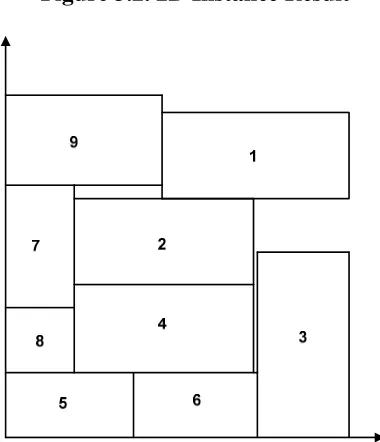
3.3. Two-dimensional Model
Although the proposed model is considered a three-dimensional knapsack problem it
can be modified in order to solve two-dimensional problems as well. The z axis
should be omitted in order to adjust the model. Since two dimensional problems are
simpler than three-dimensional ones they can be solved in a shorter time. As an
example, the instance of 4 different types of rectangles (totally 10 rectangles) is
studied. The dimensions and maximum allowed number of these rectangles are shown
in table 3.1. The dimensions of the bin, which is two dimensional as well, are equal to
Table 3.1. 2D Rectangles Dimensions and Maximum Allowed Number Rectangle type Width(mm) Height(mm) Max. allowed no.
1 229 483 4
2 165 330 3
3 165 165 1
4 229 406 1
The optimal solution is obtained after 3 hours and 37 minutes. Figure 3.1 shows the
obtained result. Compared to the three dimensional instances, the optimal solution can
be obtained sooner. However, the solution time is not reasonable for the 2D instances
as well, thus it is better to use a heuristic algorithm to reach the results in a shorter
time.
CHAPTER 4
Solution Methodology
4.1. Three Dimensional Algorithm
Based on Egeblad and Pisinger’s work (2009), the three sequences considered for the
boxes must be packed. These sequences show the relative box locations. They are
known as sequence triple. Sequence triple is one of the most successful
representations in the literature and defines the packing order. As mentioned in
Egeblad and Pisinger (2009), the sequence triple does not create all three-dimensional
packing; however, it is proved that a fully robot packable packing is obtainable with
this representation. A robot packing is a packing that can be obtained by placing
boxes from the LBB corner of the bin while each box is in-front-of, on the right side,
or above other boxes. If all six rotations of the packing are robot packable, the
packing is known as a fully robot packable packing. Although Egeblad and Pisinger
(2009) claim that their algorithm creates normalized packings, their results are not
normalized. Normalized packing is a packing when all boxes are placed as far left,
down, and back as possible without overlapping, and every new box touches an
already placed box on its left, lower, and back side. However, according to their
results some of the packed boxes are placed in the air.
The solution methodology section is organized as follows: first, sequence triple is
described in section 4.1.1 which is used in section 4.1.2 in order to place the boxes.
Simulated annealing is defined in section 4.1.3 to control the local neighbourhood
search. Orthogonal rotation, pre-placed boxes (obstacles), four-corner packing, and
box insertion order are explained in sections 4.1.4, 4.1.5, 4.1.6, and 4.1.7,
respectively.
4.1.1. Sequence Triple
Three sequences A, B, and C represent the fully robot packable packing, where A, B,
and C are permutations of the numbers 1 ... n, and n is the total number of boxes to be
placed in the bin. These sequences denote the relative placement of each of the two i
• A-chain: If box i appears before box j in the A-chain, then box i is located to the left of, on top of, or in front of box j.
• B-chain: if box i appears before box j in the B-chain, then box i is located behind, to the left of, or below, box j.
• C-chain: If box i appears before box j in the C-chain, then box i is located to the right, under, or in front of box j.
4.1.2. Placement algorithm
Based on the given three sequences, box i is located on the left side of box j if it
appears before box j in A-chain and B-chain and after box j in C-chain. Box i is
located below box j if it appears before box j in B-chain and C-chain and after box j in
A-chain. Moreover, box i is placed behind box j if it appears after box j in B-chain
and before it in A-chain and C-chain, or if box i is placed after box j in all sequences.
It is observed that box i always appears before box j in B-chain for all three given
placements. Thus, the order of placement of the boxes in the bin can be based on the
order of B-chain. The first box is placed at the origin, and the succeeding boxes are
placed according to their relative position to already packed boxes. The coordinates of
each new box are calculated based on the following formula:
)) (
, 0
max(
max
x
w
x
i= j∈Px j+ j)) (
, 0
max(
max
y
h
y
i= j∈Py j+ j)) (
, 0
max(
max
z
d
z
i j P j jz +
= ∈
where Px, Py,and Pz are the subsets of packed boxes located on the left, below, and
behind the new box. In order to consider vertical stability and reduce the gap between
the boxes, some modifications have been applied to Eglebad and Pisinger’s (2009)
procedure. These modifications are explained in the following section.
• Vertical Stability
As it is assumed that (x,y,z) coordinates of boxes and their dimensions are integer, it
coordinates of each to be packed box. The algorithm considers four corners of the
given box. If x and z coordinates of one of these corners are equal to the coordinates
of one of the points at the top of any packed box, it returns the height of that box.
Then, the y coordinate of the new box would be equal to maximum of those values.
The proposed approach is illustrated in the following:
1. Consider (xi, yi, zi)
P
yj∈
∀ : compute x’j and z’j
Where xj≤ x’j≤ xj+wj-1 and zj≤ z’j≤ zj+dj-1
If (xi = x’j and zi= z’j) then
Return yj+ hj
Else Go to 2
2. Consider (xi + wi, yi, zi)
P
yj∈
∀ : compute x’j and z’j
Where xj+1 ≤ x’j≤ xj+wj and zj≤ z’j≤ zj+dj-1
If (xi+ wi = x’j and zi= z’j) then
Return yj+ hj
Else Go to 3
3. Consider (xi, yi, zi + di)
P
yj∈
∀ : compute x’j and z’j
Where xj≤ x’j≤ xj+wj-1 and zj+1 ≤ z’j≤ zj+dj
If (xi = x’j and zi+ di = z’j)
Return yj+ hj
Else Go to 4
4. Consider (xi + wi, yi, zi + di)
P
yj∈
∀ : compute x’j and z’j
Where xj+1 ≤ x’j≤ xj+wj and zj+1 ≤ z’j≤ zj+dj
If (xi+ wi= x’j and zi+dj = z’j) then
Return yj+ hj
Else Return 0
Return
y
max(0,max
(y
h
j))j j
The algorithm pushes each packed box downward where possible such that its bottom
can be supported by the bin floor or by the top of other packed boxes.
4.1.3. Simulated annealing
Although it is relatively simple to develop a simulated annealing heuristic, choosing a
good neighborhood and cooling procedure, which itself depends on several different
parameters, is usually necessary for the algorithm to work efficiently. The cooling
procedure is different for various types of problem and even between instances of the
same problem. Therefore, it is difficult to find out a good cooling procedure. In the
proposed simulated annealing algorithm, the temperature is reduced when a new
solution is accepted, according to the following function:
t→t/(1+ βt)
where β is the cooling parameter. Besides the cooling down procedure, the process is
allowed to heat up again whenever it is appeared be getting trapped. The heating up
function is:
t→t/(1- αt)
where α is the heating parameter. The temperature is reduced when the solution is
accepted and increased when the solution is rejected. α must be smaller than β as the
number of acceptances is small relative to number of rejections (Dowsland, 1993).
The neighbourhood of each solution is defined as one of these five permutations:
either exchange two boxes from one of the sequences; exchange two boxes in
sequences A and B; exchange two boxes in sequences A and C; exchange two boxes
in sequences C and B; or exchange two boxes in all sequences. An overview of the
simulated annealing algorithm is as follows:
// Prepare the initial state and volume
temperature := initial_temperature
initial_state := randomly generated state
best_state := initial_state
while (time is not up) do
neighbours := generate_neighbourhood(best_state)
neighbour := randomly select an element from neighbours
neighbour_volume := volume_utilized(neighbour)
found_better := false
if (neighbour_volume>best_volume) then
found_better := true
else
// We accept a worse solution at random, but the chance of
// doing so decreases with the temperature.
temperature := temperature / (1+β*temperature)
delta := (best_volume – neighbour_volume) / best_volume
i := random number between 0 and 1
if (i< e^( -delta / temperature ) ) then
found_better := true
else
//increase temperature
temperature := temperature / (1-α*temperature)
end if
end if
if (found_better) then
selected := selected + 1
best_state := neighbour
best_volume := neighbour_volume
end if
end while
return best_state
The solutions are compared based on the bin utilization. The formula used for
calculating the utilization percentage is as follows:
4.1.4. Orthogonal Rotation
The boxes are allowed to be rotated orthogonally with respect to the bin. Suppose the
width, height, and depth of all boxes are respectively parallel to x, y, and z axis, and
wi, hi, and di represents the width, height, and depth of box i, respectively. It is
possible to obtain better packings if the boxes were rotated in different directions.
Egeblad and Pisinger (2009) considered box rotation only for the two dimensional
instances but neglected to include it in the three dimensional experiments. Boxes are
allowed to be rotated in one of the following orientation:
WHD: Standard orientation.
WDH: Swap the height and the depth. HWD: Swap the width and the height.
HDW: Swap the width and the height, and then swap the height with the depth. DHW: Swap the depth with the width.
DWH: Swap the depth with the width, and then swap the depth with the height.
The given rotation is applied to the simulated annealing by adding an additional
transformation to the neighbourhood generating routine. The orientation of the boxes
is generated randomly at first. Thus, an additional vector R which shows the
orientation of the boxes is stored as well as the sequence triple.
4.1.5. Obstacles
Suppose O is a set of rectangular obstacles with known coordinates (x, y, z) and
known dimensions (w, h, d). At the beginning of the algorithm, the obstacles are fixed
into the bin. The packing is created from the sequence triple and those boxes that
overlap with any obstacles in the set are removed. The container free volume is
calculated as follows:
4.1.6. Four-corner packing
Four packing schemes, one for each corner are created. First, the coordinates of the
boxes are calculated relative to the current origin. Then, their real (x, y, z) coordinates
are calculated relative to the real origin of the container which is its LBB corner. The
processing technique is as follows:
W := bin width H := bin height D := bin depth w := box width h := box height d := box depth
if (loading from front) then
// No change needed: this is the default loading method. return <x,y,z>
else if (loading from rear) then return<W – x – w, y, D – z – d> else if (loading from left side) then return<W – z – w, y, x>
else if (loading from right side) then return<z, y, D – x – w>
end if
4.1.7. Order of box insertion
As mentioned earlier, the order of inserting boxes into the container is based on
B-chain. The order of the boxes in B-chain can be created randomly or can be based on
the volume of the boxes which means ones with larger volume are packed first.
4.2. Two Dimensional Algorithm
Although the algorithm is proposed for the three dimensional knapsack problem, it
can also be used to solve two dimensional instances as solving a two-dimensional