Exploring the energy-time tradeoff in mpi programs on a power-scalable cluster

(1)

Exploring the Energy-Time Tradeoff in MPI Programs

on a Power-Scalable Cluster

Vincent W. Freeh

Feng Pan Nandani Kappiah

Department of Computer Science

North Carolina State University

{vwfreeh,fpan2,nkappia}@ncsu.edu

David K. Lowenthal

Rob Springer

Department of Computer Science

The University of Georgia

{dkl,springer}@cs.uga.edu

Abstract

Recently, energy has become an important issue in high-performance computing. For example, supercomputers that have energy in mind, such as BlueGene/L, have been built; the idea is to improve the energy efficiency of nodes. Our approach, which uses off-the-shelf, high-performance clus-ter nodes that are frequency scalable, allows energy saving by scaling down the CPU.

This paper investigates the energy consumption and exe-cution time of applications from a standard benchmark suite (NAS) on a power-scalable cluster. We study via direct mea-surement and simulation both intra-node and inter-node ef-fects of memory and communication bottlenecks, respec-tively. Additionally, we compare energy consumption and execution time across different numbers of nodes.

Our results show that a power-scalable cluster has the potential to save energy by scaling the processor down to lower energy levels. Furthermore, we found that for some programs, it is possible tobothconsume less energy and

execute in less time when using a larger number of nodes, each at reduced energy. Additionally, we developed and val-idated a model that enables us to predict the energy-time tradeoff of larger clusters.

1. Introduction

Recently, power-aware computing has gained traction in the high-performance computing (HPC) community. As a result, low-power, high-performance clusters, such as Blue-Gene/L [1] or Green Destiny [32], have been developed to stem the ever-increasing demand for energy. Such systems improve the energy efficiency of nodes. Consider the case of Green Destiny—a cluster of Transmeta processors—which consumes less energy than a conventional supercomputer. In particular, Green Destiny consumes about three times less energy per unit performance than the ASCI Q machine.

However, because Green Destiny uses a slower (and cooler) microprocessor, ACSI Q is about 15 times faster per node (200 times overall) [32]. A reduction in performance by such a factor surely is unreasonable from the point of view of many users. If performance is the only goal, then one should continue on the current “performance-at-all-costs” path of HPC architectures. On the other hand, if power is paramount, then one should use a low-performance archi-tecture that executes more instructions per unit energy.

We believe one should strike a path between these two extremes. This is conceptually possible because an increase in CPU frequency generally results in a smaller increase in application performance. The reason for this is that the CPU is not always the bottleneck resource. Therefore, increas-ing frequency also increases CPU stalls—usually waitincreas-ing for memory or communication. Consequently, there are op-portunities where energy can be saved, without an undue performance penalty, by reducing CPU frequency.

As a preliminary step, this paper studies the tradeoff be-tween power and performance (or equivalently energy and time) for HPC. In particular, this paper makestwo key

con-tributions. First, we evaluate a real, small-scale

power-scalable cluster, which is a cluster composed of proces-sors that are each frequency scalable—i.e., their clock speed and hence power consumption can be changed dynamically. This illustrates the tradeoff between the power-conserving benefits and the time-increasing costs of such a machine. Second, in order to estimate the potential for large power-scalable clusters, we developed a simulation model that al-lows us to predict energy consumed and time taken. Studies like this are needed so that architects can make informed decisions before building or purchasing large, expensive power-scalable clusters.

(2)

a simple metric that predicts this energy-time tradeoff. Ad-ditionally, we found that in some cases one can save energy

andtime by executing a program on more nodes at a slower gear rather than on fewer nodes at the fastest gear. We be-lieve this will be important in the future, where a program running on a cluster may be allowed to generate only a fixed amount of heat. Finally, this paper presents a model for es-timating energy consumption. It validates the model on a real power-scalable cluster, then extrapolates to determine the benefit of a larger power-scalable cluster.

The rest of this paper is organized as follows. Section 2 describes related work. Next, Section 3 discusses the mea-sured results on our power-scalable cluster. The next section presents our simulation results up to 32 nodes. Finally, Sec-tion 5 summarizes and describes future work.

2. Related Work

There has been a voluminous amount of research per-formed in the general area of energy management. In this section we describe some of the closely related research. We divide the related work into two categories: server/desktop systems and mobile systems.

2.1. Server/Desktop Systems

Several researchers have investigated saving energy in server-class systems. The basic idea is that if there is a large enough cluster of such machines, such as in hosting cen-ters, energy management can become an issue. In [5], Chase

et al. illustrate a method to determine the aggregate sys-tem load and then determine the minimal set of servers that can handle that load. All other servers are transitioned to a low-energy state. A similar idea leverages work in cluster load balancing to determine when to turn machines on or off to handle a given load [26, 27]. Elnozahyet al.[10] in-vestigated the policy in [26] as well as several others in a server farm. Such work shows that power and energy man-agement are critical for commercial workloads, especially web servers [3, 21]. Additional approaches have been taken to include DVS [9, 28] and request batching [9]. The work in [28] applies real-time techniques to web servers in order to conserve energy while maintaining quality of service.

Our work differs from most prior research because it focuses on HPC applications and installations, rather than commercial ones. A commercial installation tries to reduce cost while servicing client requests. On the other hand, an HPC installation exists to speedup an application, which is often highly regular and predictable. One HPC effort that addresses the memory bottleneck is given in [18]; however, this is a purely static approach.

In server farms, disk energy consumption is also sig-nificant. One study of four energy conservation schemes concludes that reducing the spindle speed of disks is the

only viable option for server farms [4]. DRPM is a scheme that dynamically modulates the speed of the disk to save energy [14, 15]. Another approach is to improve cache performance—if many consecutive disk accesses are cache hits, the disk can be profitably powered down until there is a miss; this is the approach taken by [36]. An alternative is to use an approach based on inspection of the program counter [12]; the basic idea is to infer the access pattern based on inspection of the program counter and shut down the disk accordingly. A final approach is to try to aggregate disk accesses in time. A compiler/run-time approach using this was designed and implemented in [16], and a prefetch-ing approach in [25]. Both were designed for mobile sys-tems but can be directly applied to server/desktop syssys-tems.

There are also a few high-performance computing clus-ters designed with energy in mind. One is BlueGene/L [1], which uses a “system on a chip” to reduce energy. An-other is Green Destiny [32], which uses low-power Trans-meta nodes. A related approach is the Orion Multisystem machines [23], though these are targeted at desktop users. However, using a low-power processor sacrifices perfor-mance in order to save energy.

2.2. Mobile Systems

There is also a large body of work in saving energy in mobile systems; most of the early research in energy-aware computing was on these systems. Here we detail some of these projects.

At the system level, there is work in trying to make the OS energy-aware through making energy a first class re-source [29, 8, 6]. Our approach differs in that we are con-cerned with saving energy in asingle program, not a set of processes. One important avenue of application-level re-search on mobile devices focuses on collaboration with the OS (e.g., [22, 33, 35, 2]). Such application-related ap-proaches are complementary to our approach.

In terms of research on device-specific energy savings, there is work in the CPU via DVS (e.g., [11, 13, 24]), the disk via spindown (e.g., [17, 7]), and on the memory or network [20, 19]. The primary distinction between these projects and ours is that energy saving is typically the pri-mary concern in mobile devices. In HPC applications, per-formance is still the primary concern.

3. Measured Results

(3)

130 135 140 145 150 155 160 165

900 1000 1100 1200 1300 1400 1500 1600 1700 1800 0.95 1 1.05 1.1 1.15 1.2 1.25 1 1.1 1.2 1.3 1.4 1.5 1.6 1.7 1.8 1.9 2 2.1

Energy consumption (kJ)

Execution time (s)

(a) BT B

58 60 62 64 66 68 70 72

500 550 600 650 700 0.825 0.85 0.875 0.9 0.925 0.95 0.975 1 1 1.05 1.1 1.15 1.2 1.25 1.3 1.35 1.4 1.45

Execution time (s)

(b) CG B

45 50 55 60 65

350 400 450 500 550 600 650 700 750 1 1.1 1.2 1.3 1.4 1.5 1 1.25 1.5 1.75 2 2.25 2.5

Execution time (s)

(c) EP B

150 155 160 165 170 175

1100 1200 1300 1400 1500 1600 1700 1800 1900 0.9 0.925 0.95 0.975 1 1.025 1.05 1.075 1 1.1 1.2 1.3 1.4 1.5 1.6 1.7 1.8

Execution time (s)

(d) LU B

31 32 33 34 35 36 37 38 39

250 300 350 400 0.95 1 1.05 1.1 1.15 1 1.1 1.2 1.3 1.4 1.5 1.6 1.7 1.8 1.9 2

Execution time (s)

(e) MG B

150 155 160 165 170 175

1200 1300 1400 1500 1600 1700 1800 0.825 0.85 0.875 0.9 0.925 0.95 0.975 1 1 1.1 1.2 1.3 1.4 1.5 1.6

Execution time (s)

(f) SP B

Figure 1. Energy consumption vs execution time for NAS benchmarks on a single AMD machine.

This study uses, as a reference example, a cluster of ten nodes, each equipped with a frequency- and voltage-scalable AMD Athlon-64. We run each program at each available energy gear: 2000 MHz, 1800 MHz, 1600 MHz, 1400 MHz, 1200 MHz, and 800 MHz.1_{The voltage, which} ranges from 1.5–1.0V, is reduced in each gear. Each node has 1GB main memory, a 128KB L1 cache (split), and a 512KB L2 cache, and the nodes are connected by 100Mb/s network. In this paper, we control the CPU power and mea-sure overall system energy. This is effective in saving en-ergy because the CPU—a major power consumer—uses less power. In particular, the Athlon CPU used in this study consumes approximately 45-55% of overall system energy.2 For each program we measure execution time and energy consumed for an application at a range of energy gears. Ex-ecution time is elapsed wall clock time. The voltage and current consumed by the entire system is measured by pre-cision multimeters at the wall outlet to determine the in-stantaneous power (in Watts). This value is integrated over time to determine the energy used. Integration is performed

1 The 1000 MHz does not work reliability on a few of the nodes. 2 CPU power is not measured directly. However, the system power at

the fastest energy gear is 140–150 W. The AMD datasheet states that the maximum CPU power consumption is 89 W. We estimate the peak power of the CPU for our application is in the range of 70–80 W, which is 45–55% of system power.

by a separate computer that samples two multimeters sev-eral tens of times a second.

We divide our results into two parts. First, we discuss results on a single processor. This shows the energy-time tradeoff due to the memory bottleneck. The next section shows time and energy results for the NAS suite on multi-ple nodes. This shows the effect of the communication bot-tleneck as well as the energy-time tradeoff when the num-ber of nodes increases.

3.1. Single Processor Results

Figure 1 shows the results of executing 6 NAS programs on a single Athlon-64 processor. The NAS FT benchmark is not shown because we cannot get it to work, and IS is not shown because (1) class B is too small to get any parallel speedup and (2) class C thrashes on 1 and 2 nodes, making comparative energy results meaningless. For each graph, the

(4)

not(0,0). Therefore, the alternate axes show the time and

energy relative to the fastest gear (leftmost point).

All of our tests show that for a given program, using the fastest gear takes the least time (i.e., it is the leftmost point on the graph). The greatest relative savings in energy is 20%, which occurs in CG operating at gear 5 (1200MHz). This savings incurs a delay (increase in execution time) of almost 10%. The best savings relative to performance oc-curs at gear 2 (1800MHz) which saves 9.5% energy with a delay less than 1%. On the other hand, EP at 1800MHz saves 2% energy with an 11% delay. This delay is approxi-mately the same as the increase is CPU clock cycle.

At a lower gear, a given program runs longer; if the de-crease in power exceeds the inde-crease in time, a lower gear uses less energy. We have found that the increase in time from one gear to another is bounded above and below as fol-lows:1≤ Ti+1

Ti ≤

fi

fi+1, whereTiandfiare the execution

time and frequency at geari, respectively. In words, shift-ing to a slower gear will never speed up a program, nor will it slow a program by more than the increase in CPU cycle time. This makes intuitive sense and is borne out by our em-pirical results. Further testing shows that a program with a time increase close to the upper bound has the CPU on the critical path. In other words, its performance depends on the throughput of the CPU. EP is representative of such a pro-gram. On the other hand, a program such as CG, which has a small time increase at slower gears, is largely indepen-dent of CPU frequency. Because we tested the in-core ver-sion of NAS (i.e.,class B), these programs do not have sig-nificant I/O. Therefore, programs that are not dependent on the CPU donothave the CPU on the critical path,e.g., the memory subsystem is instead on the critical path. One more test that also shows the dependency on CPU or memory is the effect the gear has on overall UPC (micro-operations per cycle). In memory-bound applications, the UPC increases as frequency decreases. This increase is because the cycle time of the processor increases, but the memory latency re-mains the same. At a lower frequency, memory latency is less in terms of CPU cycles. Consequently, there fewer de-lay slots that must be filled, and ILP increases.

We looked for a predictor of the energy-time tradeoff. The typical measure of IPC or UPC is problematic because it varies too much. The programs we consider in this sec-tion do not perform much I/O. Therefore, the memory sys-tem is the only other component that could be on the criti-cal path. The metric we chose is micro-operations per mem-ory reference (i.e., per L2 cache miss). This value stays con-stant as the frequency changes. What UPM (µop/miss)

in-dicates is the pressure exerted on the memory system by the program. Misses per cycle or per second are dependent on CPU frequency and, therefore, are not useful.

Table 1 shows the ratio UPM for the 6 NAS benchmark programs. The benchmarks are sorted from highest to low-est, ranging from a high of 844 for EP to a low of 8.60 for

UPM Slope1→2 Slope2→3

EP 844. -0.189 0.288

BT 79.6 -0.811 0.0510

LU 73.5 -1.78 -0.355

MG 70.6 -1.11 -0.161

SP 49.5 -5.49 -1.52

CG 8.60 -11.7 -1.69

Table 1. Predicting energy-time tradeoff.

CG. The next column shows the slope of the energy-time curve from the fastest gear to gear 2, computed as E2−E1

T2−T1.

A large negative number indicates a near vertical slope and a significant energy savings relative to the time delay. On the other hand, a small negative number indicates a near horizontal slope and little energy savings. The last column shows the slope from second to third gear. Except for MG, we see that the slopes are also sorted, in this case from great-est (positive) to least (negative). Because the more nega-tive slope indicates a better energy-time tradeoff, this table shows that memory pressure tends to predict the energy-time tradeoff.

3.2. Multiple Processor Results

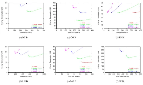
The previous section investigated the energy-time trade-off on a single node. This section studies the effect of dis-tributed programs. Figure 2 shows results from six NAS programs. Results from FT and IS are not shown for the reasons stated above. Each graph has the same general lay-out as in Figure 1, except that it shows the results from mul-tiple experiments: 2, 4, and 8 nodes (or 4 and 9 nodes in the case of BT and SP). One-node results from the previ-ous section are also plotted, but in most cases these curves are to the right window shown. The energy plotted is cumu-lative energy of all nodes used.

Before discussing the results, we describe the possible shapes of these graphs. First, for a fixed number of nodes, the shape of the curve depends on the memoryand commu-nication bottlenecks. This is because in a distributed pro-gram, not only might a processor wait for the memory sub-system, but at times it also might block awaiting a message. In either scenario, the CPU is not on the critical path, and idle or slack time is more efficiently spent at a lower en-ergy gear.

Second, consider the possible effects when comparing an experiment with2Pnodes versus one withPnodes. The

following possibilities exist. Note that we do not consider the case where the time on2P nodes islargerthan onP

nodes.

1. The curve for2P nodes can lie completely above and to the left of the curve forP nodes. Each point on the

(5)

0 50 100 150 200 250

0 100 200 300 400 500 600

Energy Consumption (KJ)

Execution time (s) 1 node

4 nodes 9 nodes

(a) BT B

0 20 40 60 80 100 120 140 160 180

0 50 100 150 200 250 300 350 400

2 nodes 4 nodes 8 nodes

(b) CG B

0 10 20 30 40 50 60 70

0 50 100 150 200 250 300 350 400

(c) EP B

0 50 100 150 200 250

0 200 400 600 800 1000

(d) LU B

0 10 20 30 40 50 60 70 80

0 50 100 150 200 250 300

(e) MG B

0 50 100 150 200 250 300 350 400

0 100 200 300 400 500 600 700 800

4 nodes 9 nodes

(f) SP B

Figure 2. Energy consumption vs execution time for NAS benchmarks on 2, 4, and 8 (or 2 and 9) nodes.

curve. This case occurs when the program achieves

poor speedupon2Pnodes compared toP nodes.

2. The point that represents the fastest energy gear for2P

nodes can be to the left, at or below, the corresponding point on the curve forPnodes. This case occurs when

the program achievesperfect or superlinear speedup

on2Pnodes compared toPnodes.

3. The curve for2Pnodes can lie to the left of the curve

forP nodes, but not completely above or below the fastest gear point forP. This is the most interesting

case. While the program executes faster and consumes more energy in the fastest gear on2P nodes than on P nodes, there is a lower gear at 2P nodes that has

less energy consumption than the fastest gear point at

Pnodes. Therefore, it is possible to achieve better

exe-cution timeandlower energy consumption by running at a lower energy gear on2P nodes than at a higher

energy gear onP nodes. There is not an energy-time tradeoff between these points because one point dom-inates the other in both energy and time. This case oc-curs case whenspeedup is good(i.e., not superlinear and not poor) and there are a significant number of main memory accesses (so that scaling down the

pro-cessor has only a slightly detrimental effect). We describe each of the cases in turn below.

Case 1: Poor Speedup

Figure 2 offers several examples of case 1. In particular, this case is illustrated in BT, SP, and MG from 2 to 4 nodes, and CG from 4 to 8 nodes.

We believe in the future a given supercomputer cluster will be restricted to a certain amount of power consumption or heat dissipation. If there is a limit for energy/power con-sumption or heat dissipation, this would be represented as a horizontal line. For programs in this case, the line will in-tersect at most one of the curves. The most desirable point would be the leftmost (fastest) one under the limit.

Case 2: Superlinear Speedup

(6)

0 20000 40000 60000 80000 100000 120000 140000 160000

0 100 200 300 400 500 600 700 800

Execution time (s) 2 nodes

4 nodes

6 nodes

8 nodes 10 nodes

Figure 3. Energy consumption vs. execution time for Jacobi iteration on 2, 4, 6, 8, and 10 nodes.

speedup the energy consumption decreases as nodes are added. When speedup is perfect or superlinear there is no energy-time tradeoff, because the energyandtime are never better with fewer nodes.

Case 3: Good Speedup

Figure 2 shows several examples of this case. First, con-sider LU at 4 and 8 nodes. Gear 4 on 8 nodes uses approx-imately the same energy as the fastest gear on 4 nodes, but executes 50% more quickly. The fastest gear on 8 nodes executes 72% faster than on 4 nodes, but uses 12% more energy. This case illustrates an additional choice not avail-able in a conventional cluster, which only supports either the fastest gear option (4 or 8 nodes). So a user must trade off a performance increase against an energy increase. With a power-scalable cluster, the user can select a slower gear on 8 nodes, which may offer better performance for the same energy consumption. Thus, a user of a power-scalable clus-ter has two dimensions to explore: (1) number of nodes and (2) processor performance gear. In case 3, the user may be able to get better performance by using more nodes, with each node executing at a lower energy gear.

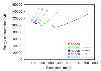
Next, Figure 3 plots data for a (hand-written) Jacobi it-eration application. This application is shown because it can run at any number of nodes, unlike the NAS bench-marks. The figure shows energy-time curves on 5 configu-rations: 2, 4, 6, 8, and 10 nodes. Because this application gets good speedup (1.9, 3.6, 5.0, 6.4, and 7.7) each adja-cent pair of curves falls in case 3. For example, executing in second or third gear on 6 nodes results in the program fin-ishing slightly fasterandusing less energy than using first gear on 4 nodes.

Finally, we present results from a synthetic benchmark. This benchmark models CG in terms of its cache miss rate, but achieves good speedup (over 7 on 8 nodes). The

0 10000 20000 30000 40000 50000 60000 70000 80000 90000 100000

0 50 100 150 200 250 300 350 400 450

4 nodes

8 nodes

Figure 4. Synthetic benchmark with high memory pressure.

pose of this benchmark is to show the potential of a power-scalable cluster. Figure 4 shows the results. Because the miss rate is high (7%), the execution time penalty for scal-ing down is low (e.g., 3% at gear 5, 1200MHz), and the corresponding energy savings is large (e.g., 24% at gear 5). Furthermore, compared to gear 1 on 4 nodes, gear 5 on 8 nodes uses 80% of the energy and executes in half the time.

4. Simulated Results

The previous section presented results on up to ten power-scalable nodes. While the results are encourag-ing, it is left unclear what performance (in time and energy) can be expected for larger power-scalable clus-ters. Most likely, before building or buying a large power-scalable cluster, one would like to determine the per-formance potential. As we do not have access to more than ten nodes, this section seeks to address this issue by devel-oping a simulation model.

4.1. Model

Understanding scalability of parallel programs is of course a difficult problem; indeed, it is one of the fun-damental problems in parallel computing [30, 31]. Re-searchers try to predict scalability using a range of tech-niques, from analytical to execution-based. We will use a combination of both.

(7)

reliable results from a larger non-power-scalable cluster.) To determine time and energy on slower gears, we measure power consumption on a cluster node and use a straight-forward algebraic formula. Below we describe our five-step methodology in full detail.

Step 1: Gather time traces. The first step is to gather active and idle times onnnodes (TA₍_n₎_and_TI₍_n₎_{, respectively,}

whereTI₍_n₎_{includes the actual communication time) on}

each of our clusters. This includes the (ten-node) power-scalable cluster described above as well as a 32-node Sun cluster.3 _{The parameter} _n _{varies to include all} configura-tions on which the NAS suite can run. We gather the traces at only the fastest gear on the power-scalable cluster, and the Sun cluster is not power scalable. We decompose the to-tal execution time intoTA₍_n₎_and_TI₍_n₎_{by instrumenting}

MPI. This instrumentation intercepts all relevant MPI calls, and writes a timestamp to a log file.

For all MPI communication routines used in each bench-mark, interception functions report the time at which the routine was entered and exited. These operations create a trace from which we recover active and idle times. To re-duce perturbation, each trace record is written to a local buffer.

Step 2: Model computation and communication. The sec-ond step is to develop a model of computation and commu-nication that is based onTA₍_n₎_and_TI₍_n₎_{. This will help}

us predict (in step 3)TA₍_m₎_and_TI₍_m₎_where_{m >}₁₀_,_i.e_,

for power-scalable configurations with more than ten nodes. Our approach here is distinct for each quantity, out of neces-sity: no matter what the gear, the power consumed is differ-ent when computing than when blocking awaiting data. The formulas below do not mention gear because all of these measurements are taken at thefastestgear.

DeterminingFpandFs. Here, we use Amdahl’s law to

estimateFpandFs, which denote the parallelizable and

in-herently sequential fractions of an application, respectively. For a test withinodes, we estimateFpandFsas follows:

TA₍_i_{) =} _TA₍₁₎₍_F

p/i+Fs)

Fp = 1−Fs

We obtain a family ofFpandFsvalues. We will use these to

determineFpandFson large power-scalable clusters. Also,

TA₍_n₎_{represents the}_maximum_{computation time over all}

nodes.

Classifying communication. Here, we recall thatTI

in-cludes idle time and communication time. While idle time (due to load imbalance) can be directly derived fromTA_,

the communication cost cannot. Hence, our approach is to categorize communication of each NAS program into one of three groups: logarithmic, linear, or quadratic. These are

3 We also ran tests on a 64-node Xeon cluster, but as the network was shared among several large jobs, the results were unreliable.

three common scaling behaviors for communication. To do this, we rely on three complementary methods: (1) inspec-tion of the behavior of our measured TI _{on up to nine}

power-scalable nodes, (2) dynamic measurement of num-ber of each MPI call as well as inspection of corresponding source code, and (3) the literature in the field (e.g., [34]). Specifically, we classified communication in BT, EP, MG, and SP as logarithmic; CG as quadratic, and LU as linear.

Step 3: Extrapolation ofTA₍_m₎_and_TI₍_m₎_{at fastest gear.}

Third, we extrapolate to 16, 25, and 32 power-scalable nodes,i.e.,m > 10. For a given number of nodes,m, the

sum ofTA₍_m₎_and_TI₍_m₎_{yields the execution time.}

Predicting active time: PredictingTA₍_m₎_{, requires an}

appropriateFp andFs for 16 and 32 nodes on the

power-scalable cluster. Using our measured values on up to 32 nodes on the Sun cluster and up to 9 nodes on our power-scalable cluster, we fitFp andFsfor 16, 25, and 32 nodes

on the power-scalable cluster using a linear regression.

Predicting idle time: Given the classification of

commu-nication behavior (logarithmic, linear, or quadratic) for each application, we use regression to fit a curve to the commu-nication using measured data on power-scalable nodes. This gives us communication time on 16, 25, and 32 nodes.

Validation. Our technique is validated in the following

way. ForTA₍_m₎_{, we compared}_F

pandFson up to 9 nodes

on both clusters. With only 1 exception, it was identical; the outlier was CG, where the parallelism actually increases from 4 to 8 nodes on our power-scalable cluster, but is con-stant on the Sun cluster. ForTI₍_m₎_{, each communication}

shape that we chose for our power-scalable cluster is identi-cal on the Sun cluster up to 32 nodes. We also note that [34] supports our conclusion on five of the six programs. The ex-ception is LU; for this program, we found that communica-tion was best modeled as a constant; our traces showed that when nodes are added, each node sends more messages, but the average message size decreases.

Armed with estimates ofTA₍_m₎_and_TI₍_m₎ _{on larger}

configurations (at the fastest gear), we now turn our atten-tion to determining the effect of different energy gears on execution time and energy consumption. The last two steps in this methodology are concerned with this issue.

Step 4: DetermineSg,Pg, andIg. The next step is to gather

power data from a single power-scalable node. Two values will be needed on a per-application and per-gear basis: ap-plication slowdown (Sg) and average power consumption

(Pg). Separately, the power consumption for an idle (i.e.,

inactive) system is determined for each gear (Ig).

This data determines the increase in time and the de-crease in power. The execution time for a sequential pro-gram is wall clock time. This is done foreach(sequential) program at each energy gear. The ratio Sg is determined

as follows:Sg = Tg(1)_T₁−(1)T1(1). Now that we are discussing

(8)

at gearg.

The valuesPgandIgare obtained by measuring overall

system power. The voltage and current consumed by the en-tire system is measured at the wall outlet to determine the instantaneous power (in Watts), as described in Section 3. This experimental setup determines the values,Pg, for each

application and for each gear. The same setup, except this time with no application running, was used to determine the power usage of an idle system (Ig) at each gear.

Step 5: Determine Tg(m) and Eg(m). The final step is

to estimate the time and energy consumption of a power-scalable cluster using the information developed so far. The time for a lower gear is computed by increasing the active time by the appropriate ratio,Sg. We assume that

execut-ing in a reduced gear does not itself increase the idle time, as our experimentation has shown that the time for com-munication is independent of the energy gear—the compu-tational load during MPI communication is quite low. Us-ing the values ofPg andIg, we can estimate energy

con-sumption at each lower gear for the MPI program. In this straightforward case, the time and energy estimates, onm

nodes, for each gear are:

Tg(m) = SgTA(m) +TI(m) (1)

Eg(m) = PgSgTA(m) +IgTI(m). (2)

At slower gears the compute time is greater than that of the fastest gear, whereas the idle time is independent of the gear. Thus the time executing in geargincreases toSgTA.

Communication latency is independent of gear, so this is as-sumed to remain the same.

However, this naive case above is too simple because it assumes all computation is on the critical path. In many pro-grams, not all computation is on the critical path. Of course, reducing the energy gear of any computation on the crit-ical path will delay other nodes, who must wait for data sent from the (now slower) node. In the refined model,TA

is classified into whatcriticalandreduciblework (TC_and

TR_{), and in our estimates of computation we separate these}

and estimate each. In short, executing reducible work in a slower gear mightnotincrease overall execution time, be-cause an increase in the time of reducible work will de-crease the idle time. On the other hand, executing critical work in a slower gear always increases execution time. The communication latency, which is unaffected by CPU fre-quency, is delayed only by the slowdown applied to the crit-ical work. The idle time is slack for the reducible work. However, if reducible work is slowed such that all slack is consumed, then the time will be extended. This point of in-flection is whenTR₊_TI ₌_S

gTR.

The post-processing analysis conservatively determines the reducible work to be computation between thelast send4

4 We assume that the send is asynchronous.

and a blocking point. In between those two points there is no interaction between nodes, so the work is not on the criti-cal communication path. With this refinement, Equation (1) changes as shown below. Note that for notational simplic-ity, we omit number of nodes (m).

Tg=

Sg(TC+TR), ifTI+TR≤SgTR

Sg(TC+TR) +TI+TR−SgTR,otherwise

Then, Equation (2) becomes

Eg=

 



PgSg(TC+TR), ifTI+TR≤SgTR

PgSg(TC+TR) +Ig(TI+TR−SgTR),

otherwise

Assumptions The methodology described in this section makes use of two assumptions. First, this methodology as-sumes that the power consumed when an application is computing is constant (because we use the average power). This is reasonable as the observed power consumption for regular applications is fairly constant (within a few percent). Second, it assumes that the power consumption follows a step function, in that at all times the power consumed is ei-therPg orIg. In reality, the transition takes between these

power levels takes some time. However, this time is negli-gible, and the transition occurs on both sides of an idle pe-riod, tending to equal out.

4.2. Evaluation

Figure 5 shows the results of our simulation on each ap-plication ranging from 2–32 nodes. All node configurations up to and including 9 nodes are actual runs on the cluster, and configurations of 16, 25, and 32 nodes are simulated us-ing the model discussed previously.

In the same way that the eight- and nine-node tests tend to be more “vertical” than the two- and four-node tests, as with the runs up to nine nodes, the shapes of the graphs tend to become more “vertical” when using 16, 25, or 32 nodes;

i.e., using lower gears becomes a better idea. As an exam-ple, consider SP. On four nodes, second gear consumes the least energy. On the other hand, on 16 nodes, fourth gear consumes the least energy.

One possible implication of this is that for massively par-allel power-scalable clusters, the individual nodes can be placed in a relatively low energy gear with only a modest time penalty. As discussed in the previous section, this may potentially allow for supercomputing centers to fit more nodes in a rack while staying within a given power bud-get. On the other hand, this could degrade performance sig-nificantly if many applications for such machines are em-barrassingly parallel.

(9)

0 50 100 150 200 250 300 350 400

0 100 200 300 400 500 600

(a) BT B

0 50 100 150 200 250 300 350 400 450

0 50 100 150 200 250 300 350 400

(b) CG B

0 10 20 30 40 50 60 70 80

0 50 100 150 200 250 300 350 400

4 nodes 8 nodes 16 nodes 32 nodes

(c) EP B

0 50 100 150 200 250 300

0 100 200 300 400 500 600 700 800 900 1000

(d) LU B

0 20 40 60 80 100 120 140 160 180

0 50 100 150 200 250 300

(e) MG B

0 100 200 300 400 500 600 700

0 100 200 300 400 500 600 700 800

(f) SP B

Figure 5. Simulated energy consumption vs execution time for NAS benchmarks on up to 32 nodes.

the total cluster energy consumed starts to increase dramat-ically. Essentially, continuously increasing the number of nodes causes an application to be placed in the poor speedup classification (see previous section), which we know is en-ergy inefficient. Also, for each application, there exists a certain number of nodes that, if exceeded, will cause pro-gram slowdown. It appears that that point is around 32 nodes for the NAS suite on our power-scalable Athlon-64 cluster.

This problem is not unique to power-aware computing; indeed, it is a problem with roots in the scalability field. However, it is clear that when this phenomenon occurs, it is necessarily the case that communication dominates compu-tation. This means that in fact a lower gear is almost certain to be better. Hence, if one does not know what the paral-lel efficiency for a given application is, using a lower en-ergy gear is a safeguard against excessive enen-ergy consump-tion.

5. Conclusions and Future Work

This paper has investigated the tradeoff between energy and performance in MPI programs. We have studied trends on both one processor and multiple processor programs. Us-ing the NAS benchmark suite, we found for example that on one node, it is possible to use 10% less energy while in-creasing time by 1%. Additionally, we found that in some cases one can save energyandtime by executing a program

on more nodes at a slower gear rather than on fewer nodes at the fastest gear. We believe this will be important in the fu-ture, where a cluster may have heat limitations.

The reason why energy saving is possible is because of delays in the processor, where executing at a high frequency and voltage do not make the program execute faster, but does waste energy. This delay is due to (1) the processor waiting for the memory system to fetch a value or (2) the processor blocking awaiting a message from a remote pro-cessor.

(10)

Acknowledgments

This research was supported in part by NSF award CCF 0234285. We give special thanks to Dan Smith for some of the low-level software and comments on early versions of the paper.

References

[1] N. Adiga et al. An overview of the BlueGene/L supercom-puter. InSupercomputing 2002, Nov. 2002.

[2] M. Anand, E. Nightingale, and J. Flinn. Self-tuning wireless network power management. InMobicom, Sept. 2003. [3] P. Bohrer, E. Elnozahy, T. Keller, M. Kistler, C. Lefurgy,

C. McDowell, and R. Rajamony. The case of power man-agement in web servers. In R. Graybill and R. Melham, edi-tors,Power Aware Computing. Kluwer/Plenum, 2002. [4] E. V. Carrera, E. Pinheiro, and R. Bianchini. Conserving disk

energy in network servers. InProceedings of International Conference on Supercomputing, pages 86–97, San Fransisco, CA, 2003.

[5] J. S. Chase, D. C. Anderson, P. N. Thakar, A. Vahdat, and R. P. Doyle. Managing energy and server resources in host-ing centres. InSymposium on Operating Systems Principles, pages 103–116, 2001.

[6] C. C. Corporation, I. Corporation, M. Corporation, P. T. Ltd., and T. Corporation. Advanced configuration and power in-terface specification, revision 2.0. July 2000.

[7] F. Douglis, P. Krishnan, and B. Bershad. Adaptive disk spin-down policies for mobile computers. In Proc. 2nd USENIX Symp. on Mobile and Location-Independent Com-puting, 1995.

[8] C. Ellis. The case for higher-level power management. In

Proceedings of the 7th Workshop on Hot Topics in Operating Systems, March 1999.

[9] E. Elnozahy, M. Kistler, and R. Rajamony. Energy conserva-tion policies for web servers. InUSITS ’03, 2003.

[10] E. M. Elnozahy, M. Kistler, and R. Rajamony. Energy-efficient server clusters. InWorkshop on Mobile Comput-ing Systems and Applications, Feb 2002.

[11] K. Flautner, S. Reinhardt, and T. Mudge. Automatic performance-setting for dynamic voltage scaling. In Pro-ceedings of the 7th Conference on Mobile Computing and Networking MOBICOM ’01, July 2001.

[12] C. Gniady, Y. C. Hu, and Y.-H. Lu. Program counter based techniques for dynamic power management. InProceedings of the 10th International Symposium on High-Performance Computer Architecture, Feb. 2004.

[13] D. Grunwald, P. Levis, K. Farkas, C. Morrey, and M. Neufeld. Policies for dynamic clock scheduling. In Pro-ceedings of 4th Symposium on Operating System Design and Implementation, October 2000.

[14] S. Gurumurthi, A. Sivasubramaniam, M. Kandemir, and H. Franke. Dynamic speed control for power management in server class disks. InProceedings of International Sympo-sium on Computer Architecture, pages 169–179, June 2003. [15] S. Gurumurthi, A. Sivasubramaniam, M. Kandemir, and

H. Franke. Reducing disk power consumption in servers with DRPM.IEEE Computer, pages 41–48, Dec. 2003.

[16] T. Heath, E. Pinheiro, J. Hom, U. Kremer, and R. Bianchini. Application transformations for energy and performance-aware device management. InProceedings of the 11th In-ternational Conference on Parallel Architectures and Com-pilation Techniques, Sept. 2002.

[17] D. P. Helmbold, D. D. E. Long, and B. Sherrod. A dynamic disk spin-down technique for mobile computing. InMobile Computing and Networking, pages 130–142, 1996.

[18] C.-H. Hsu and U. Kremer. The design, implementation, and evaluation of a compiler algorithm for CPU energy reduc-tion. InACM SIGPLAN Conference on Programming Lan-guages, Design, and Implementation, June 2003.

[19] R. Krashinsky and H. Balakrishnan. Minimizing energy for wireless web access with bounded slowdown. InMobicom 2002, Atlanta, GA, September 2002.

[20] A. R. Lebeck, X. Fan, H. Zeng, and C. S. Ellis. Power aware page allocation. InArchitectural Support for Programming Languages and Operating Systems, pages 105–116, 2000. [21] C. Lefurgy, K. Rajamani, F. Rawson, W. Felter, M. Kistler,

and T. W. Keller. Energy management for commerical servers.IEEE Computer, pages 39–48, Dec. 2003.

[22] R. J. Minerick, V. W. Freeh, and P. M. Kogge. Dynamic power management using feedback. InWorkshop on Com-pilers and Operating Systems for Low Power, pages 6–1–6– 10, Charlottesville, Va, Sept. 2002.

[23] O. Multisystems. http://www.orionmulti.com/.

[24] B. D. Noble, M. Satyanarayanan, D. Narayanan, J. E. Tilton, J. Flinn, and K. R. Walker. Application-aware adaptation for mobility. InProceedings of the 16th ACM Symposium on Operating Systems and Principles, pages 276–287, October 1997.

[25] A. E. Papathanasiou and M. L. Scott. Energy efficiency through burstiness. InWMCSA, Oct. 2003.

[26] E. Pinheiro, R. Bianchini, E. V. Carrera, and T. Heath. Dy-namic cluster reconfiguration for power and performance. InCompilers and Operating Systems for Low Power, Sept. 2001.

[27] E. Pinheiro, R. Bianchini, E. V. Carrera, and T. Heath. Load balancing and unbalancing for power and performance in cluster-based systems. InWorkshop on Compilers and Op-erating Systems for Low Power, Sept. 2001.

[28] V. Sharma, A. Thomas, T. Abdelzaher, and K. Skadron. Power-aware QoS management in web servers. In24th An-nual IEEE Real-Time Systems Symposium, Cancun, Mexico, Dec. 2003.

[29] A. Vahdat, A. Lebeck, and C. Ellis. Every joule is precious: The case for revisiting operating system design for energy ef-ficiency.SIGOPS European Workshop, 2000.

[30] J. S. Vetter. Performance analysis of distributed applications using automatic classification of communication inefficien-cies. InInternational Conference on Supercomputing, pages 245–254, May 2000.

[31] J. S. Vetter and M. McCracken. Statistical scalability analy-sis of communication operations in distributed applications. InPrinciples and Practice of Parallel Programming, pages 123–132, June 2001.

[32] M. Warren, E. Weigle, and W. Feng. High-density comput-ing: A 240-node beowulf in one cubic meter. In Supercom-puting 2002, Nov. 2002.

[33] M. Weiser, B. Welch, A. J. Demers, and S. Shenker. Schedul-ing for reduced CPU energy. InOperating Systems Design and Implementation (OSDI ’94), pages 13–23, 1994. [34] F. C. Wong, R. P. Martin, R. H. Arpaci-Dusseau, and D. E.

Culler. Architectural requirements and scalability of the NAS parallel benchmarks. InProceedings of Supercomput-ing ’99, Portland, OR, Nov. 1999.

[35] H. Zeng, C. S. Ellis, A. R. Lebeck, and A. Vahdat. Currentcy: Unifying policies for resource management. In USENIX 2003 Annual Technical Conference, June 2003.