Efficient Implementation of MIMO Detectors for Emerging Wireless Communication Standards.

ABSTRACT

NARIMAN MOEZZI MADANI. Efficient Implementation of MIMO Detectors for Emerging Wireless Communication Standards. (Under the direction of Professor W. Rhett Davis).

MIMO (Multi-Input Multi-Output) wireless systems have been widely used in next-generation wireless systems, such as 802.11n, LTE (long-term evolution), and WiMAX. The use of multiple antennas at the transmitter and receiver significantly increases data throughput without utilizing additional bandwidth or transmission power. The extraction of the signal from the spatially multiplexed transmitted streams is a complex process. Many baseband signal processing algorithms have been developed, but sphere decoders are the most popular due to their near ML performance while achieving lower power and complexity. The K-best algorithm which is one of the three types of SDs (fixed complexity sphere decoder, depth-first, and K-best) exhibits a fixed throughput while providing a BER performance close to ML in different SNRs. Furthermore, the K-best algorithm is very amenable for soft-output detection because it inherently generates the candidate list required to calculate the LLR (log-likelihood ratio) values for soft-output detection.

However, K-best designs in the literature use a multi-stage architecture that is not reconfigurable for different antenna configurations. Furthermore, the area of conventional multi-stage architectures increases quadratically with the number of antennas, reducing its efficiency for large antenna arrays.

architecture, the three-dimensional child reduction technique is proposed, which by discarding the un-necessary branches reduces the complexity of the detector. To eliminate the throughput bottle-neck of this architecture the parallel merge algorithm/architecture is proposed, which provides the shortest critical path among other merge architectures.

Efficient Implementation of MIMO Detectors for Emerging Wireless Communication Standards

by

Nariman Moezzi Madani

A dissertation submitted to the graduate faculty of North Carolina State University

in partial fulfillment of the requirements for the degree of

Doctor of Philosophy

Electrical Engineering

Raleigh, North Carolina August 2010

APPROVED BY:

_______________________________ ______________________________ Dr. W. Rhett Davis Dr. Paul D. Franzon

Committee Chair

ii

BIOGRAPHY

iii

ACKNOWLEDGEMENTS

I would like to summarize my acknowledgement to the people who have been supporting and collaborating with my work. Without them, this dissertation would never have been accomplished. I am so grateful to be a part of an innovative project, a friendly group, and an enjoyable working environment. Please allow me thank the people who gave me this opportunity.

First and foremost, I would like to thank my family: my parents, Mansooreh and Feridoun, and my brothers, Kaveh and Goudarz. Their love and support have been my source of inspiration, power, and ambition. Even the physical distance between my family and I has been greater, I can feel a stronger tie linking us together. Without them, I could not imagine how I could ever be able to manage all the difficulties and challenges.

I would like to thank my advisor and friend, Dr. W. Rhett Davis, who brought me into the VLSI world and confronted me with real design issues and solutions. He also has guided me through my study and career path. I have always enjoyed the conversations with him in both academia and other topics.

iv

I would like to specially thank my colleague and friend Thorlindur Thorolfsson for his smart advices and collaboration during the design and synthesis of the work. Without him and his efforts none of the implementation results could be achieved.

Next, I would like to take this chance to thank my colleagues and friends. I would like to thank Samson Melamed and Chris Mineo for their generous support. They have provided all the complementary materials to facilitate my research during my stay. It is always a great pleasure to work with smart people. I also would like to thank Ravi Jenkal from whom I learned a lot about MIMO detectors, which helped me greatly during the different phases of my research.

v

TABLE OF CONTENTS

LIST OF FIGURES...vii

LIST OF TABLES...ix

1.

INTRODUCTION TO MIMO ...1

1.1. INTRODUCTION... 1

1.2. WHY MIMO? ... 1

1.3. MOTIVATION... 2

1.4. MIMOTYPES... 2

1.5. OPTIMUM DETECTION SOLUTION... 3

1.6. ALTERNATIVE MIMODETECTION ALGORITHMS... 5

1.6.1. Linear Detection... 5

1.6.2. Interference Cancellation... 6

1.6.3. Lattice Reduction Aided Technique ... 6

1.6.4. Fixed-Complexity Soft-Output (FCSO)... 7

1.6.5. Sphere Decoders... 8

1.7. REVIEW OF THE MIMODETECTOR IMPLEMENTATIONS... 13

1.8. SUMMARY... 15

1.9. ORGANIZATION OF DOCUMENT... 15

2.

HARD-OUTPUT K-BEST SD...17

2.1. INTRODUCTION... 17

2.2. PRE-PROCESSING TECHNIQUES... 17

2.2.1. Real Value Decomposition (RVD) ... 18

2.2.2. Sorted QR Decomposition (SQRD)... 20

2.3. K-BEST ARCHITECTURE... 21

2.4. K-BEST UNITS... 24

2.4.1. MCU ... 24

2.4.2. Merge Unit... 27

2.4.3. Increment Calculation Unit... 28

2.4.4. Trace Back ... 29

2.5. THROUGHPUT BOTTLENECK... 31

2.5.1. Sort algorithms... 31

2.5.2. Merge Algorithms/Architectures ... 32

A. Motivation ... 32

B. Merge Architectures... 32

2.6. PARALLEL MERGE BLOCK... 34

2.6.1. Parallel Merge Algorithm... 34

2.6.2. Parallel Merge Architecture ... 36

2.6.3. Simulation Results ... 38

2.6.4. Implementation Results... 39

2.7. COMPLEXITY REDUCTION (MODIFIED K-BEST) ... 40

2.7.1. Three Dimensional Child Reduction... 41

2.7.2. Implementation Results... 45

2.8. CONCLUSION... 46

vi

3.1. INTRODUCTION... 47

3.2. SOFT-OUTPUT DETECTION... 47

3.3. K-BEST SOFT-OUTPUT DETECTION... 50

3.3.1. LLR Clipping... 51

3.4. IMPROVED CHANNEL-PROCESSING TECHNIQUE (MMSE-SQRD)... 52

3.4.1. Performance Results... 52

3.4.2. Complexity Comparison... 53

3.5. ARCHITECTURE... 55

3.6. IMPLEMENTATION RESULTS... 56

3.7. CONCLUSION... 57

4.

IN-PLACE ARCHITECTURE ...58

4.1. INTRODUCTION... 58

4.2. IN-PLACE ARCHITECTURE... 60

4.3. RECONFIGURABILITY... 61

4.4. THROUGHPUT... 62

4.5. DESIGN CONSIDERATIONS FOR THROUGHPUT INCREASE... 63

4.5.1. Partial-Sort-Bypass ... 63

4.5.2. Symbol Interleaving... 67

4.5.3. Multi-Core Architecture... 69

4.6. IMPLEMENTATION RESULTS... 70

4.6.1. Soft-output In-Place Architecture... 70

4.6.2. Comparison to Other Sphere Decoders ... 71

4.6.3. In-Place Vs. Multi-Stage: LTE and 802.11n Standards ... 73

4.7. CONCLUSION... 74

5.

DETECTOR IMPLEMENTATION FOR 64-QAM

CONSTELLATION...75

5.1. ARCHITECTURE... 75

5.1.1. Removing Shift Registers, and embedding ICU in MCU... 75

5.1.2. Trace Back Unit... 77

5.1.3. LLR Calculator... 77

5.2. SIMULATION RESULTS... 78

5.3. CHILD REDUCTION... 79

5.3.1. Simulation Results ... 79

5.3.2. Determining the Surviving Children... 80

5.3.3. Throughput... 82

5.4. IMPLEMENTATION RESULTS... 84

5.4.1. Original K-best Versus Modified K-best... 84

5.4.2. Comparison to Other Detectors ... 85

5.5. CONCLUSION... 87

6.

CONCLUSION...89

vii

LIST OF FIGURES

Figure 1. A possible implementation of depth first algorithm. ...11

Figure 2. An example of K-best algorithm (K = 4) for a 3*3 QPSK MIMO system. ...12

Figure 3. An example of the FSD algorithm. ...12

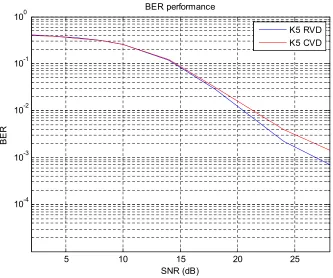
Figure 4. BER comparison: RVD vs. CVD...19

Figure 5. BER comparison of QRD and SQRD with ZF estimation. ...21

Figure 6. The simplified multi-stage architecture...22

Figure 7. Parallel architecture for the PE. ...23

Figure 8. Sequential architecture for the PE...23

Figure 9. Block diagram of each PE. ...25

Figure 10. The MCU circuit. ...26

Figure 11.Conceptual diagram for ordering ej based on the signs...27

Figure 12. Proposed ICU architecture...29

Figure 13. Trace back method. ...30

Figure 14. Trace back circuit diagram. ...31

Figure 15. One cycle merge unit with K = 3 [20]...33

Figure 16. 1 A 4*4 odd-even merging block...34

Figure 17. An example for the proposed PMA...36

Figure18. 3 by 3 parallel merge architecture...37

Figure 19. BER performance for the 4x4 16QAM hard-output MIMO detector for K=5 and 8 and ML. ...39

Figure 21. The tree structure after the second modification...44

Figure 22. The tree structure after the third modification. ...44

Figure 23. Modified K-best strategy which results to BER close to K8 after implementation considerations. ...44

Figure 24. BER comparison between ML, K8 and modified K8 in AWGN channel. ...45

Figure 25. System block diagram. ...49

Figure 26. MIMO Detection process ...50

Figure 27. The detector implementation results for K = 5, K = 8 and K =10. ...54

Figure 28. BER comparison for ML, K5-MMSE, K10-ZF, K12-ZF and K14-ZF. ...54

Figure 29. BER comparison for different algorithms. ...55

Figure 30. Architecture for a 4 by 5 odd-even merge network. ...56

Figure 31. a) Multi-stage architecture b) in-place architecture. ...59

Figure 32. Area increase with number of antennas...59

Figure 33. The simplified circuit diagram of the in-place architecture...61

Figure 34. Elimination of bubbles using partial-sort-bypass technique and K =5. a) original architecture where the pipeline in MCU generates two bubbles b) partial-sort method eliminates one bubble c) Bypass strategy eliminates the other bubble...64

viii

Figure 36. Partial-sort-bypass (circuit shown red) and symbol interleaved (shown in blue)

strategies applied to the in-place architecture...67

Figure 37. Multi-core structure...69

Figure 38. Estimated area for the designs in different technologies...70

Figure 39. The circuitry for the new ICU...76

Figure 40. Modified in-place architecture...77

Figure 41. Soft-output computation unit. ...78

Figure 42. MMSE-SQRD vs. ZF-SQRD for 2x2 64-QAM. ...79

Figure 43. Modified K-best vs. original K-best...81

Figure 44. Exploring the first three constellation nodes. ...81

ix

LIST OF TABLES

Table 1. Complexity comparison of complex and real domain K-best algorithm for K = 5,

without considering sorting complexity. ...20

Table 2. Ordering the PEDs based on e_i signs. ...27

Table 3. Complexity comparison of merge algorithms...37

Table 4. Tradeoff between complexity and BER performance of the system...38

Table 5. ASIC implementation results for 4*4 16QAM MIMO detectors based on K-best algorithm...40

Table 6. Comparison between the number of operations in the original K-best ...46

Table 7. ASIC implementation results for 4*4 16QAM MIMO detectors. ...46

Table 8. ASIC implementation results for 4*4 16QAM sphere decoders...57

Table 9. ASIC Implementation Results for 4*4 16-QAM MIMO Detectors...71

Table 10. Complexity comparison; K-best vs. modified K-best ...82

Table 11. Power consumption of the original and modified K-best units using the single-core architecture @ 284MHz ...83

1

1.

Introduction to MIMO

1.1.

Introduction

There is an increasing interest to raise the wireless data rates beyond Gigabit-per-Second to provide users with mobile access to high-bandwidth data, voice, and video applications regardless of their locations. The first draft of the standard IEEE 802.11n for wide-area wireless networks was originally designed to offer 100Mbps, but the need for a faster system was felt; therefore, the second draft is offering 600Mbps. There are other emerging standards and projects which are targeted to reach a data rate of 1Gbps such as IEEE 802.16m (Gbps WiMax [1]) and WIGWAM (Wireless Gigabit with Advanced Multimedia Support [3]). Also, the data rates even go higher in Wireless Personal Area Networks like IEEE 802.15.3c standard which offers data rates up to 15Gbps. MIMO is the solution or one of the solutions to these standards. In a MIMO system multiple antennas are deployed at transmitter as well as receiver. In the next subsection it is stated that why MIMO technology is used to increase the data rates.

1.2.

Why MIMO?

2

constraints. MIMO technology increases the data rate just by using multiple transmit and receive antennas all working at the same frequency and without using additional transmit power.

1.3.

Motivation

Two problems exist with current soft-output sphere decoders: IP reusability is one of the real concerns in the industry, and designing a reconfigurable IP which can work with different number of antennas and constellations in run-time, yet being efficient in terms of area/power/throughput is very important which has not been addressed yet. Also, the current designs in the literature are not very practical for the MIMO based standards and their provided throughput and area are both more than what are expected by these standards. By using the K-best algorithm combined with my proposed parallel merge architecture (PMA), the child reduction technique and the MMSE-SQRD channel processing technique, I have designed a low-area in-place reconfigurable architecture for 16QAM and 64QAM constellations. Also, using a multi-core architecture is the solution for a reconfigurable system which supports large number of antennas, that we have incorporated in our design.

1.4.

MIMO Types

3

diversity: open-loop and closed-loop techniques. In the open-loop, no channel information is used when transmitting the signal from the antennas. Redundant copies of one stream of data will be coded using techniques called space-time coding and transmitted from multiple antennas. Space time Codes (STC) subdivide into two main categories: Space Time Trellis Codes (STTC) which distribute a trellis code over multiple antennas and multiple time-slots and provide both coding gain and diversity gain. The other type is Space Time Block Code (STBC) which transmits multiple copies of a data stream across a number of antennas and to exploit the various received versions of the data to improve the reliability of data-transfer.

Closed-loop diversity techniques instead use the channel information, like transmit beamforming techniques where proper magnitude and phase weights computed from the channel estimation are re-applied across antennas to aim the signal in a given desired direction [2].

Spatial multiplexing is another type of MIMO, which the transmitter transmits different streams of data independently from multiple antennas within a single frequency band and the signal will be received by multiple antennas at the other side. The data capacity of the system then grows directly in line with the number of antennas. In this work we have considered the spatial multiplexing feature of MIMO systems. Next section includes the mathematical review of MIMO channel and different solutions in the literature.

1.5.

Optimum Detection Solution

4

implementation, other algorithms are also used which are introduced in the next section. Considering a MIMO system with M transmit and N receive antennas, the received signal will be:

n Hs

y= + (1)

Where H is the channel matrix, whose elements represent the complex transfer functions from the transmit antenna to the receive antenna, and are all i.i.d. complex zero-mean Gaussian with variance 0.5 per dimension. S is the M array transmitted signal with each element from a complex constellation o and n is N dimensional i.i.d. Gaussian noise with variances_n2. We can assume that channel estimation techniques are used and the channel matrix H is known. The mathematically optimal solution to find vector S from received vector y is called the Maximum Likelihood (ML):

(2)

ML is an exhaustive search over all the possible constellations in_oM_{. The space that ML}

searches is over ₂MQ _{candidates which is dependent to the number of the constellation points} Q and transmit antennasM. The vector which makes the norm in (2) the smallest is the most

reliable answer. The implementation of ML for a 4*4 QPSK system is feasible but it is not for 16QAM or higher constellation points. For example for a 4*4 16QAM system 216 vectors need to be tried. Among MIMO detection algorithms (zero-force, MMSE, V-BLAST, SD) sphere decoders (SDs) have attracted more interest because of their lower complexity and

2

||

||

min

arg

ˆ

y

Hs

s

=

5

near ML performance. There is a brief introduction of the most popular algorithms for MIMO detection in this section.

1.6.

Alternative MIMO Detection Algorithms

1.6.1. Linear Detection

The simplest solution is to suppress the interference between different layers by multiplying both sides of the equation (1) by matrix G followed by a parallel symbol decision on all layers[5]. This strategy is also called nulling:

Gn GHs GY

yˆ= = + (3)

One method to define matrix G is the Zero-Force equalization, which simply finds the transmitted symbol just using the inverse of the channel matrix in case of a square channel matrix or using the Moore-Penrose pseudo-inverse in case of a nonsquare matrix:

H H

ZF H H H H

G ₌ + _{=( )}-1 ₍₄₎

This results to a very low hardware implementation of the detector, but suffers from the performance degradation due to the enhanced noise term. This problem can be alleviated by another linear detection method that takes the receiver noise into account: Minimum Mean Square Error (MMSE) equalization exploits the extended channel matrix

H M n H M n

ZF _I H H I H

H H

G ₍ 2 ₎-1

6

Where s_n is the variance of the noise at the receive antenna and I_Mis the M by M identity matrix. The draw back of reducing the noise enhancement is some remaining interference between layers[6].

1.6.2. Interference Cancellation

The linear detection methods can not eliminate the interference between layers effectively, so Interference Cancellation methods were introduced to improve the performance of the detection. The two main variants of this technique are: Parallel Interference Cancelation (PIC) and Successive Interference Cancellation (SIC). PIC has shown a good performance in very high diversity environments but not in environments which space is the main source of diversity. SIC has shown better performance compared to PIC and was the base for the original BLAST detectors [6]. The detection process happens layer by layer in the way that after detecting a layer, the interference of this layer will be removed from all other layers before detecting the next layer. This technique needs QR decomposition to be able to detect the signals layer by layer.

1.6.3. Lattice Reduction Aided Technique

7

algorithm are low quality. So this technique is attractive when low uncoded BERs are targeted [6].

1.6.4. Fixed-Complexity Soft-Output (FCSO)

The FCSO MIMO detector is presented in [7] and uses a suboptimal method ZF-DFE to reduce the complexity of the ML algorithm. Each complex symbol is considered as one layer and only the top layer is exactly marginalized and the remaining layers are approximately marginalized. This process happens for each layer, so for a 4x4 system happens 4 times. This algorithm like sphere decoders, needs two separate processes. Firstly the channel-rate processing of FCSO happens, which includes the QR decomposition of M ranked reduced channel matrices Hk:

Hk= [h1,…,hk-1,hk+1,…,hm] (6)

Which produces the upper triangular matrices Rk and the unitary matrices Qk for each k as

Hk = Qk Rk (7)

Therefore M QR decompositions have to happen. The other process is the symbol-rate processing which includes finding the log-likelihood ratio (LLR) values for each bit, which consists the following steps:

1. One of the symbols si iÎ{1,...,M}is chosen as the top layer. The entire constellation O is enumerated (64 constellations for 64-QAM). For each candidate the effect of this layer should be removed from the received vector. Considering the kth candidate it will happen in the following way:

k i is h r

8 2. By multiplying rˆ with H

k

Q from (7), compute

r Q

r H

k ˆ

~_{= (9)}

3. Based on rˆ and R, and exploiting DFE the rest of the symbols s2,s3,…,sM can be estimated using hard decision. After finding these symbols the LLR for the bits in the first layer can be computed by

2

ˆ ˆ _{k b}

k = r-R s

d (10)

To find the LLR for the rest of the bits, each symbol should be place at the top layer and the same processes to happen again.

1.6.5. Sphere Decoders

As stated before, ML is the best mathematically solution for MIMO detection. But the implementation of this algorithm is costly and impractical. QR decomposition will reduce the complexity of ML by changing the problem to a tree search and pruning process. Consider matrix H = QR, in which R is an upper triangular and Q is a unitary matrix. Multiplying both sides of (1) by QH will result to:

where y_{ˆ =}QHy ₍₁₁₎

This leads to solving the following:

) ( min arg

ˆ d s

s= where _{d(s)=|| yˆ-Rs||}2 ₍₁₂₎

) (s

d can be rewritten as a recursive sum of Partial Euclidian Distances (PED) or metrics:

2

1 i

i

i d e

d = ₊ + where d(s)=d₁,d_M+1 =0 (13)

ˆ H

y Rs Q n= +

M

9 and distance increments are:

2 2

ˆ

å

=

-= M

i j

j ij i

i y R s

e (14)

Equation (13) can be mapped to a tree search with metric dM+1 in the root and metric d1 in the leaves. Each stage of the tree reveals a candidate symbol. For example in stage i of the tree

M i

s s s

si _{[ i, i ,..., M], 1,2,...,}

1 =

10 1.6.5.1. Depth First

The Schnorr-Euchner (SE) enumeration is a depth first algorithm which was the first algorithm adapted in the state of the art implementations[8]. In this method search starts from the root and moves towards down and right while the radius C is unknown yet. When a leaf node is reached, the algorithm updates the radius C= d(s)to the square root of the new metric. So by adaptive adjusting the sphere radius the process of pruning happens faster. Figure 1 shows a possible implementation of the depth first algorithm. The gray circles show the nodes which their metric is calculated and the black circles show the leaves which are candidates for being the ML solution. The black circle with the smaller metric shows the path which is the ML solution.

11

Figure 1. A possible implementation of depth first algorithm.

1.6.5.2. Breadth First (K-best)

K-best is a breadth-first SD search that instead of expanding all of the nodes in each stage of the tree expands only the K nodes (parents) that have the smallest PEDs (metrics). Each parent node has Q children, where Q is the constellation size. The number of the PEDs in each stage after expansion will be KQ, which just K smaller ones will survive after sorting. In the final stage the node with the smallest PED will reveal the ML vector by tracing back this node towards the root. Figure 2 shows an example of the K-best algorithm. The gray circles show the survived nodes in the tree.

Advantages and disadvantages: K-best SD has a fixed throughput and is simple to implement. The performance of the system is mostly dependent to the parameter K. Choosing higher Ks will result in a BER close to ML. The problem is that by increasing the parameter

12

Figure 2. An example of K-best algorithm (K = 4) for a 3*3 QPSK MIMO system.

1.6.5.3. FSD

FSD algorithm starts the tree search with expanding all of the children in the first stage and expanding just the first child of these expanded nodes in the next levels (Figure 3). FSD[14] provides high throughput data rate because this algorithm is highly pipelinable, but the complexity and power consumption of this algorithm is high. Also the error-rate performance of this algorithm in SNRs less than 20dB is low compared to other algorithms. COSIC [15] reduces the complexity of FSD but still suffers from the same BER problem. Also this algorithm doesn’t provide good quality soft-outputs for coded systems.

13

1.7.

Review of the MIMO Detector Implementations

14

techniques. In [43] [43], the authors introduced a K-best architecture that works for different values of K during the run-time in order to reduce power consumption. Kim in [38] implemented a soft-output 4x4 QPSK K-best detector with LDPC iterative coding; however, the implementation of a 4x4 QPSK system is much easier than a higher constellation. Authors in [42] proposed the bounded soft sphere detection (BSSD) algorithm where the search bounds are used based on the distribution of the number of candidates found inside the sphere. In [44], Bhagawat designed a reconfigurable detector based on layered orthogonal decoding (LORD) for different constellation sizes.

To the best of our knowledge, the only work implementing a sphere decoder supporting different antenna configurations was developed by Yang [45] and Amiri [46] Both designs implement the hard-output detector and are based on depth-first and FSD, respectively. In fact, soft-output detection is a rather challenging case compared to the hard-output detection. Barbero in [47] shows that soft-output extension of the FSD algorithm requires major modifications of the algorithm, which will increase the complexity of the FSD. Yang in [45] divides the tree into sub-trees to enable reconfigurability and multi-core design. This conversion reduces the BER performance of the depth-first algorithm, which makes this design inefficient, especially when used for soft-output detection.

15

1.8.

Summary

MIMO detection process and different solutions in the literature were introduced. The ML solution is too complex and impractical for hardware implementation. The linear detection methods have the problem of enhancing noise in the detection process. The nulling-cancellation method has a better performance than linear methods but the complexity is high, because the inverse of the channel matrix needs to be calculated repeatedly. The Sphere Decoders have shown to have a performance close to the ML solution maintaining less complexity to the other algorithms in the same error-rate regime. The K-best SD is the algorithm that based on my simulations and implementations is the most promising solution for MIMO detection, and also the target of this work.

1.9.

Organization of Document

16

17

2.

Hard-Output K-best SD

2.1.

Introduction

In this section the designed architecture for the K-best algorithm is introduced. Before introducing the architecture, there are some points needed to be explained regarding the processes applied to the received signal before the detection process. The process applied to the received signal before the signal detection is called pre-processing or channel processing where the QR decomposition happens. The QR decomposition can be combined with two other processes which will result in a better BER performance of the sphere decoder. Two well-known pre-processing techniques are real value decomposition and sorted QR decomposition. After introducing the pre-processing techniques the K-best architecture is introduced. This architecture uses the conventional multi-state architecture, and our contribution to this design is proposing the parallel merge algorithm and the parallel merge architecture to remove the throughput bottleneck of the K-best designs. As shown later the data rate (throughput) of the K-best architectures is limited by the merge architecture, and the throughput decreases with an increase in parameter K. The proposed parallel merge architecture has a short critical path which does not increase with parameter K.

2.2.

Pre-processing Techniques

18

decoder. As introduce in the previous sections, for tree search the channel matrix H has to be decompose to the unitary matrix Q and the upper triangular matrix R. Because the circuit performing this operation is common between all the sphere decoders, the hardware implementation of this block is not a part of this work and I refer the readers to [11] for more information regarding the hardware implementation of the pre-processing unit. Before the QR decomposition RVD can be applied to the estimated complex channel matrix H to exchange all the complex values with real values in order to reduce the complexity of the sphere decoder while the sorted QR decomposition can happen in parallel with QR decomposition.

2.2.1. Real Value Decomposition (RVD)

The original received signals in the receiver are in the complex domain as shown in (1). The complex equation (1) can be rewritten as:

ú û ù ê ë é Á Â + ú û ù ê ë é Á Â ú û ù ê ë é Â Á Á -Â = ú û ù ê ë é Á Â } { } { } { } { } { } { } { } { } { } { n n s s H H H H y y

where all the signals are in real domain. After QR decomposition of the complex signals there will be M stages in the tree for an MxN antenna structure. This method will increase the number of tree levels from M to 2M and decrease the number of children for each node from

19

each stage the number of children is less, and obviously choosing K candidates out of the total K. Qchildren has a better result than choosing K candidates out of K.Q children. Second, by using RVD a smaller K will produce the same performance. And because a smaller K parameter is used, the sort block is implemented with less complexity and a smaller critical path. The sort operation is the throughput bottleneck of the K-best architectures; this advantage helps the architecture to have a higher data rate by simplifying the sort block. Finally, fewer mathematical operations are needed. For example a complex multiplication needs 4 real multiplications and 3 real additions. Table 5 shows the number of multiplications and additions performed for a 4*4 16-QAM MIMO system for both complex and real domain values with K = 5.

5 10 15 20 25

10-4 10-3 10-2 10-1 100

SNR (dB)

B

ER

BER performance

K5 RVD K5 CVD

20

Table 1. Complexity comparison of complex and real domain K-best algorithm for K = 5, without considering sorting complexity.

Algorithm Real multiplications Real Additions

K = 5, complex 512 1392

K = 5 , real 140 456

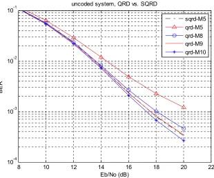
2.2.2. Sorted QR Decomposition (SQRD)

21

8 10 12 14 16 18 20 22

10-4 10-3 10-2 10-1

Eb/No (dB)

BER

uncoded system, QRD vs. SQRD

sqrd-M5 qrd-M5 qrd-M8 qrd-M9 qrd-M10

Figure 5. BER comparison of QRD and SQRD with ZF estimation.

2.3.

K-best Architecture

22

The popular architecture used in all the K-best designs, is a multi-stage architecture, where one stage is considered for each layer of the tree, as sown in Figure 6. This figure shows the simplified architecture for a 4x4 antenna configuration. As described in the previous section RVD increases the number of the layers from 4 to 8. One processing element is needed for each stage. The PEs can be designed in different ways with different complexity/performance tradeoffs. They can be divided into two categories: parallel and sequential architectures.

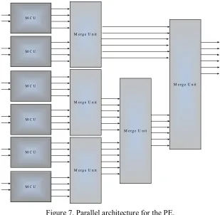
Figure 7 shows the parallel architecture for the PE. This architecture assumes that K is equal to six. Each MCU produces the PEDs for one parent. The PEDs generated in the MCUs can be pre-sorted inside this module as shown later. Therefore to sort the 6x4 = 24 PEDs and select the K smallest ones, 5 merge units in three levels are required. Each PE in this architecture contains a lot of blocks and it results in a huge area in each PE and the whole detector as well. Although this architecture provides a very high-throughput system, but a need for such a throughput does not exist and is not even predicted in the future.

Another possible architecture for the PE is the sequential architecture shown in Figure 8. This architecture uses just one MCU and one merge unit inside the PE. The MCU unit and the merge unit are used K times consecutively to produce the PEDs and sort them. This architecture consumes K-fold less area than the parallel PE architecture and yet provides a high data rate.

PE1 PE2 . . . PE8

23

M C U

M C U

M C U

M C U

M e rg e U n it

M e rg e U n it

M e rg e U n it M C U

M C U

M e rg e U n it

M e rg e U n it

Figure 7. Parallel architecture for the PE.

Merge Unit MCU

Flip-Flops

24

2.4.

K-best Units

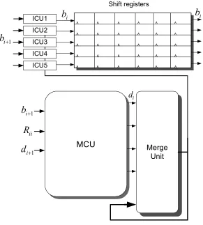
We choose the sequential architecture for implementation. The K-best sphere decoder is made of four units. Each PE includes three units which are MCU, merge unit and the increment calculator unit (ICU), and the fourth unit is the trace-back which makes a decision based on the survived candidates from different layers. These units are explained individually in this section.

2.4.1. MCU

In the previous section we explained that MCU and the merge unit are the two main blocks in the K-best sphere decoder. MCU calculates the PEDs of each parent based on equations (13) and (14). We can rewrite (14) in a new form:

2 1

2

i ii i

i

b

R

s

e

=

-

å

+ =

+ =

-M

i j

j ij i

i y R s

b

1

1 ˆ (16)

Since

b

25

adder and a shifter. The details of the MCU are shown in Figure 10. As shown in the figure, each MCU calculates children for one parent node. The diagram of the MCU unit is shown in Figure 10.

Merge Unit

MCU

i d ICU1

ICU2 ICU3 ICU4 ICU5

i

b

Shift registers

1 +

i

b

ii

R

1 +

i

d

i

b

1 +

i

b

Figure 9. Block diagram of each PE.

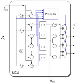
26

as it can be seen they have the di+1 term in common and the only different part is e_i 2. Therefore e_i 2 needs to be pre-sorted. To calculate the PEDs we have to calculate (15) for

} 3 , 1 , 1 , 3 {- - + + Î

s , but to sort the calculated PEDs we need to calculate e_i for } 2 , 1 , 0 , 1 , 2 {- - + + Î

s where for s=0the equation does not need a calculation because we already have calculated bi+1. The signs of the calculated e_ivalues show how to sort them.

Table 2 shows the order of e_ibased on the signs.

ii

R

-+

| |2

| |2

| |2

2 ´ Pre-sorter 1 + i b 1 + i d 2 ´ 3 ´ 3 ´ i d

Figure 10. The MCU circuit.

27

Table 2 where b_i+1 is located between ‘Rii’ and ‘0’. From the diagram, the closest point to

1

+

i

b out of {-3R_ii,-R_ii,R_ii,3R_ii} is Rii, and then –Rii, 3Rii and -3Rii which means that the order of the symbols who result in the smallest PED is : Rii , -Rii , 3Rii , -3Rii which also matches the ordering results on the left hand side of the row 4 of the table.

-3Rii -Rii 0 Rii 3Rii

1

e

3

e

e

e

2Rii

-2Rii

Figure 11.Conceptual diagram for ordering ej based on the signs.

Table 2. Ordering the PEDs based on e_i signs.

Symbol order from left to right bi+1-(Rii).(-2) bi+1-(Rii).(-1) bi+1 bi+1-(Rii).(1) bi+1-(Rii).(2)

+3 , +1 , -1 , -3 + + + + +

+1 , +3 , -1 , -3 + + + + -

+1 , -1 , +3 , -3 + + + - -

-1 , +1 , -3 , +3 + + - - -

-1 , -3 , +1 , +3 + - - - -

-3 , -1 , +1 , +3 - - - - -

2.4.2. Merge Unit

28

of the system, and so has a significant effect on the system throughput. We have compared and talked about these algorithms in the next section.

2.4.3. Increment Calculation Unit

This unit removes the effect of the currently detected symbol from the other layers. We broke (14) into (15) and (16) and stated that MCU computes (15), and ICU computes (16). It is possible to compute this equation before hand (before the time the numbers are needed) because during the process of the current level, i, this equation just needs the values from previous levels, M,…,i+1. Therefore after finding the candidates for the current level we can start calculating (15) for the next level of the tree. To find the last symbol (s1), b2 needs to be calculated based on (16):

8 18 7 17 6 16 5 15 4 14 3 13 2 12

2 yˆ R s R s R s R s R s R s R s

b = _i - + + + + + + (17)

29 + ICU ju i u u j s R

y

å

This unit is enabled for j = 1,2, …, i-1 where i shows the current layer

From merge unit5

[1:0] [3:2]

j yˆ

Figure 12. Proposed ICU architecture.

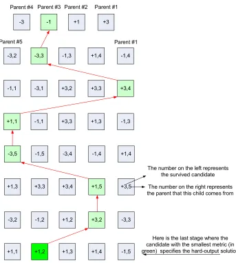
2.4.4. Trace Back

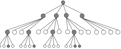
In the last stage of the tree, the candidate with smallest metric reveals the hard-output detected symbol. This solution is most probably the ML solution. The last symbol is discovered but we also need to find the other symbols. Therefore a module is needed to restore the survived candidates from other layers. Also we need to add more data to each candidate to be able to trace it from the last detected layer; one way to mark the candidates is through their parents. For example for K = 5, this number can be anything from 1 to 5. Therefore after the survived candidates are determined in each stage, the number of the parent associated with the candidate will be attached to it and the whole value will be restored in flip-flops until the end of the tree process.

30

shows that how this module works. In this example the detected vector is {-1,-3,+3,+1,-3,+1,+3,+1}. In this diagram, each rectangle shows one survived candidate, and the green rectangles show the final ML solution. The left number inside each square shows the symbol, and the number on right shows the parent number. Figure 14 shows the circuit diagram for this module.

-3 -1 +1 +3

-3,2 -3,3 -1,3 +1,4 -1,4

-1,1 -3,1 +3,2 +3,3 +3,4

+1,1 -1,1 +3,3 +1,3 -1,3

-3,5 -1,5 -3,4 -1,4 +1,4

+1,3 +3,3 +3,4 +1,5 +3,5

-3,2 -1,2 +1,2 +3,2 -3,3

+1,1 +1,2 +1,3 +1,4 -1,5

Here is the last stage where the candidate with the smallest metric (in green) specifies the hard-output solution

The number on the left represents the survived candidate

The number on the right represents the parent that this child comes from Parent #1

Parent #2 Parent #3

Parent #4

Parent #5 Parent #1

31

Par ent #

Sym bol

3 1 1

S1 S2 S2 S2 S2 S2 S3 S3 S3 S3 S3 S4 S4 S4 S4 S4 S7 S7 S7 S7 S7 S6 S6 S6 S6 S6 S5 S5 S5 S5 S5 S8 S8 S8 S8 S8 Hard-Output Solution

Figure 14. Trace back circuit diagram.

2.5.

Throughput Bottleneck

2.5.1. Sort algorithms

32 2.5.2. Merge Algorithms/Architectures

A. Motivation

The selection of the parameter K has a great effect on the throughput and the error-rate performance of the system. K = 5 with ZF-SQRD provides a 0.4dB loss at SNR 20dB compared to the ML solution, while the loss with K = 8 decreases to 0.1dB. The problem is that a higher K increases the complexity of the merge/sort algorithm. As shown in Figure 9, the data generated by the merge unit needs to be forwarded to the input ports again to be compared against the other input ports. It is not practical to use pipeline registers in the merge unit, because it will reduce the throughput of the system proportional with each additional pipeline level. Therefore the type of merge algorithm employed will have a strong effect on the throughput of the system.

B. Merge Architectures

33

comparators as the parameter K (Figure 15), and lots of logics between. This critical path noticeably reduces throughput of the K-best circuit when K increases.

Figure 15. One cycle merge unit with K = 3 [20].

34

a1 A

B L H A B L H A B L H A B L H A B L H A B L H A B L H A B L H A B L H a3 a2 a4 b1 b3 b2 b4 c1 c2 c3 c4 c5 c6 c7 c8

Figure 16. 1 A 4*4 odd-even merging block.

Parallel merge algorithm (PMA) has the shortest critical path among the explored merge algorithms, less than half of the delay of an odd-even merge algorithm according to our experiments. PMA’s critical path is independent to the parameter K. As a result, the PMA enables us to exploit a deep-pipeline architecture which results in a high-throughput system. The next section introduces the parallel merge algorithm.

2.6.

Parallel Merge Block

2.6.1. Parallel Merge Algorithm

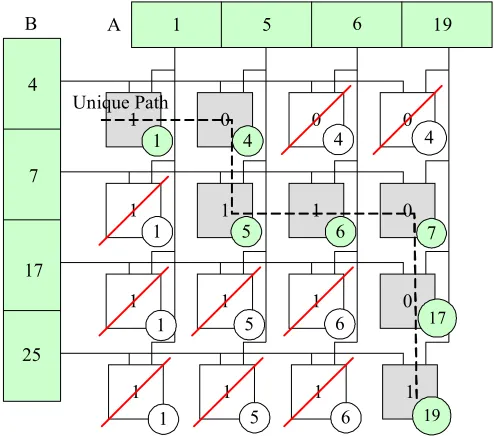
PMA merges two already sorted sequences into one output sequence in one step of parallel comparators and decision logic. The algorithm includes three steps:

1) Parallel comparison for all possible pairs from the two input sequences, providing the minimum value and a decision bit for each pair.

2) Finding the unique path which reveals the critical comparators by eliminating redundant comparators, using the decision bits.

35

The basic element in PMA is a comparator with two outputs. The first one is MIN(A,B) and the other one is a decision bit which determines if input A is smaller than input B. The logic for decision bit is:

0 1

)

(A< B D= else D=

if (18)

The algorithm is more explained in the following example. To merge two sequences

3 2 1 0,a,a ,a

a and b0,b1,b2,b3where a0 <...<a3 and b0<...<b3we put sequences A and B on

horizontal and vertical axes, in a way that a₀ and b0 are the closest together as shown in

Figure 17. In this diagram comparators are shown by squares with their first output, MIN(A,B), in a circle at the right-bottom corner of the square and the second output, decision bit, at the center of the square. This algorithm requires a comparator for each pair of

) ,

(aÎA bÎB .

36

outputs; the eighth output will be the maximum of a4 and b4. This example can be extended to merge two sequences with different number of inputs.

The complexity comparison of merge algorithms in terms of area and speed is shown in Table 3. Parallel merge provides a short and constant delay compared to odd-even merge and one-cycle merge at the expense of larger area.

0 0 0 1 0 1 1 1 0 1 1 1 1 1 1 1 1 4

5 6 7

17

19

1 5 6 19

4 7 17 25 1 1 1 5 5 6 6 4 4 A B Unique Path

Figure 17. An example for the proposed PMA.

2.6.2. Parallel Merge Architecture

37

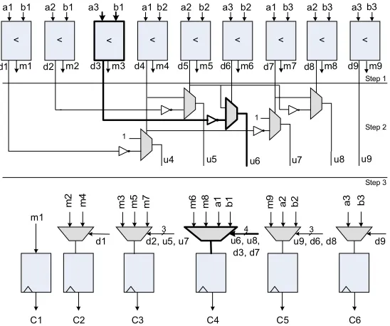
longest path of the circuit (shown in bold) goes through a comparator, an inverter, one MUX and a transmission gate. This makes the critical path of PMA the shortest among all of the other merge algorithms explored. This architecture results in a maximum clock frequency of 270MHz for K = 8 compared to 89MHz in[21] in the same technology process.

a1 b1 d1 < a2 b1 d2 < a3 b1 d3 < a1 b2 d4 < a2 b2 d5 < a3 b2 d6 < a1 b3 d7 < a2 b3 d8 < a3 b3 d9 < m1 m 2 m 4

u4 u5 u6 u7 u8 u9

d1 d2, u5, u7

m 3 m 5 m 7 u6, u8, d3, d7 m 6 m 8 a

1 _b1

u9, d6, d8

m

9

a

2 _b2 _a3 _b3

d9

C1 C2 C3 C4 C5 C6

Step 1

Step 2

Step 3 1

1

m1 m2 m3 m4 m5 m6 m7 m8 m9 <

3 4 3

Figure18. 3 by 3 parallel merge architecture.

Table 3. Complexity comparison of merge algorithms. Merge Algorithm Area Delay

Odd-even O(NlogN) O(logN)

One-cycle O(N ) O(N )

Parallel ( 2)

N

38 2.6.3. Simulation Results

We simulated a 4x4 16-QAM MIMO un-coded MIMO system with AWGN channel. The simulation results for K = 5 and 8 and ML are shown in Figure 19. The summary of the simulation results are shown in Table 4. In this table the dB loss compare to the ML curve is calculated for SNR = 20dB. As K increases the dB loss decreases, but this decrease diminishes as K gets higher. The results show that by a change from K = 7 to K = 8, a dB loss equal to 0.08 is obtained, while a change from K = 8 to K = 9 brings just 0.01dB improvement. The reason that we should be careful about choosing the right K is that, a small dB loss in hard-output systems can result in a big dB loss when non-iterative soft-output detection is used. At the same time we are not interested in consuming more power or area by choosing a big K. Therefore K = 8 provides the best complexity/performance tradeoff. Because increasing K more than this value does not change the performance significantly.

Table 4. Tradeoff between complexity and BER performance of the system.

K 10 9 8 7 6 5

39

5 10 15 20 25

10-4 10-3 10-2 10-1 100

SNR (dB)

B

ER

BER performance for 4x4 16QAM RVD-SQRD hard-output systems K5 K8 ML

Figure 19. BER performance for the 4x4 16QAM hard-output MIMO detector for K=5 and 8 and ML.

2.6.4. Implementation Results

40

Table 5. ASIC implementation results for 4*4 16QAM MIMO detectors based on K-best algorithm.

Reference [21] Proposed

Technology (µm) 0.25 0.25

Algorithm/K-best K = 8 K = 8 K = 8

Sort algorithm One-cycle merge Odd-Even PMA

Gate Count (KG) 136 145 164

Throughput (Mbps) 133 250 540

Maximum clock frequency (MHz) 66.5 125 270

Normalized Gain (Mbps/KG) 1 1.76 3.36

2.7.

Complexity Reduction (Modified K-best)

K-best SD has a fixed throughput and is simple to implement. The BER performance of the system is mostly dependent to the parameter K, which is defined as the number of the survival nodes in each stage of tree pruning. The problem is that by increasing the parameter

K, area and power consumption increase too. In addition with a higher K, sort operation gets more complicated and the detector throughput will decrease exponentially.

The early-pruning method proposed in [26] reduces the complexity of K-best. The idea is to eliminate candidates that are unlikely to become ML solution at early stages using a

bound i

K

i _T

T

41

in [27] to reduce the algorithm complexity. The drawbacks for both of these algorithms is that the nature of the algorithm is dynamic which needs a complex controller, does not eliminate any resources, and results in a variable throughput because K changes all the time. The proposed algorithm in this section is called three dimensional child reduction (3DCR) and will reduce the complexity of the system effectively. It reduces parameter K in the lower levels, and also reduces the number of children. This results in a fixed throughput and eliminating resources such as adders and multipliers and other gates effectively in the design.

2.7.1. Three Dimensional Child Reduction

The complexity of K-best algorithm can be alleviated by reducing the number of the processed nodes. Processed node is a node in the tree whose PED will be calculated during the detection process of a vector. We have reduced the number of processed nodes in the tree in 3 dimensions:

· In the original K-best, after sort operation in each stage of the tree, K nodes will survive, where K is a fixed number. It is unnecessary to keep K the same for all the stages. We can not lower parameter K in the first 3 stages, because it will result in huge performance reduction. But after stage 3 the difference between the PED of the children gets larger and larger, which means just the very first candidates will survive b y the end of tree. This will result in reducing K as the detection process gets closer to the leaves, i.e. a K = 7 can be used for stage 5 and K = 5 can be used for stage 4.

42

process will be eliminated. We can rely on this information and eliminate the children in each stage that would have been most probably eliminated in the sort process. For example in stage 5 it is possible to prune the last children, and in stage 3 to eliminate the last 2 children in the search process (Figure 21). In this way we have reduced the number of multiplications and also the sort operation will be easier.

· In the K-best algorithm, a sort operation takes place to select the first K candidates with lowest PEDs out of QK for the next stage, because the first candidates after sorting are more likely to be in the ML path. The same thing happens for their children. The children for the first candidates are more likely to be the answer than the children for the last candidates. So in each stage, the number of children can decrease for the last parents. For example in stage 5 withK=8, the number of children can change by this rule [3 3 3 3 2 2 2 2] which implies that the number of children for the last 4 parents (right ones) is less than the number of candidates for the first four parents (left ones).

43

and the modified best. As this figure shows the BER results for K8 and the modified K-best are so close and they differ just 0.03dB at SNR = 20dB.

4 4 4 4 4 4 4 4 4 4 4 4 4

4 4 4 4 4 4 4 4 4 4 4 4 4

4 4 4 4 4 4 4 4 4

4 4 4

8 7 6 5 4 3 2 1

stage

44 4 4 4 4 4 4 4 4 4 4 4 4 4

3 3 3 3 3 3 3 3 3 3 3 3 3

2 2 2 2 2 2 2 2 2

1 1 1

8 7 6 5 4 3 2 1 stage

Figure 21. The tree structure after the second modification.

4 4 4 4 4 4 4 4 4 3 3 3 3

3 3 3 3 2 2 2 3 3 3 2 2 2

2 2 2 1 1 2 2 1 1

1 1 1

8 7 6 5 4 3 2 1 stage

Figure 22. The tree structure after the third modification.

4 4 4 4 4 4 4 4 4 3 3 3 3 3 3 3 3 2 2 2 2

3 3 3 3 3 3 3 2 2 2 2 2

2 2 2 2 1 1 1 1 First stage (root)

with 4 children

Last stage (leaves) with 1 child

8 7 6 5 4 3 2 1 stage

45

12 14 16 18 20 22 24

10-3 10-2 10-1

SNR(dB)

B

ER

K8 Modified k8 ML

Figure 24. BER comparison between ML, K8 and modified K8 in AWGN channel.

2.7.2. Implementation Results

Table 6 compares the number of addition and multiplication operations needed to process a symbol vector in the original K-best algorithm and the modified one. Operations like multiplication by the constellation points (3, 1, -1, -3) and comparison are included in the additions because both can be performed by adders.

46

by 20% due to the 44% reduction in the number of operations compared to our first design which just utilizes PMA. This architecture has the same throughput as K8.

Table 6. Comparison between the number of operations in the original K-best and the modified K-best.

Number of additions Number of multiplications Number of processed

K-best, K = 8 1335 212 212

Modified 830 111 111

Table 7. ASIC implementation results for 4*4 16QAM MIMO detectors.

Reference [20] Proposed

Technology (µm) 0.25 0.25

Algorithm/K-best K = 8 K = 8 K = 8 Modified

K-Best Sort algorithm One-cycle merge Odd-Even

merge

PMA PMA

Gate Count (KG) 136 145 164 131

Throughput (Mbps)

133 250 540 540

dB Loss compared to ML at SNR =20

0.1 0.1 0.1 0.13

Maximum clock frequency (MHz)

66.5 125 270 270

2.8.

Conclusion

47

algorithm/architecture (PMA) can increase the throughput of the system up to 4 times compared to the fastest implemented K-best detector in the literature. Also the 3-dimentional child reduction technique reduces the number of operations which results in about 47% reduction in the total number of mathematical calculations.

3.

Soft-Output Detection

3.1.

Introduction

In this chapter the performance complexity of the K-best algorithm is studied in the context of coded transmission. In this type of detection, the decoder has to produce reliability information for each bit. Hard output detector can not produce this kind of information, so we will use a soft-output detector which is intended to produce the most reliable information for decoding. Soft-output detection can be used in two categories of non-iterative and iterative detection. Non-iterative detection is the focus of this work. Also we have shown that by using MMSE-SQRD (minimum mean square error- sorted QR decomposition) channel processing technique which is ignored by the majority of the sphere decoder designers, the complexity of the detector can reduce effectively.

3.2.

Soft-Output Detection

48

to M_c-QAM signal constellation and after IFFT transformation, broadcasts the data independently from M transmit antennas. The signal received by N antennas is y:

n Hs

y= + (19)

Where H is the channel matrix, and S is the M array transmitted signal where each element of

S is individually chosen from a complex constellation

o

M.M_c bits where Mc is the number of constellations. A new vector set, X, which is

associated with bit-level vector S can be defined as

X

=

[x

,

x

,

¼

,

x

]

For a coded system a posteriori probability (APP) of each bit needs to be calculated:

] 1 [ ] 1 [ ln ) ( y x P y x P y x L k k k

D ₌

-+ =

= (20)

This term is equal to the extrinsic Log-Likelihood ratio (LLR) values in a non-iterative system. With the Max-log approximation [29], the LLR-value denoted as L(.) becomes:

1 1 2 2

min

min

)

(

-=

j x X

X x

j

y

Hs

y

Hs

x

L

(21)

where +1

j

X and -1

j

49

performance but a great reduction on the calculations. The calculated LLR will be passed to the soft-input hard-output Viterbi decoder to generate the decoded bits.

The L-values in (21) need to be calculated for each bit. One of the two terms in this equation

is always the ML solution,

s

vector which its jth bit is the inverse of the ML solution bit, XML j

X

s

Î

The conceptual diagram of the soft-output MIMO detection is shown in Figure 26.The pre-processing unit provides the decomposed matrixes Q and R for the sphere decoder. The sphere decoder generates the candidate list for the LLR computation unit and this unit provides the soft-information for the channel decoder.

scrambler Convolutional

Encoder S/P

Block Interleaver

QAM

Mapping IFFT Upconversion

Block Interleaver

QAM

Mapping IFFT Upconversion

. . . Input Data De-scrambler Viterbi Decoder P/S Block De-interleaver

FFT _conversionDown

. .

.

output

Data _Output

Soft-MIMO Detector FFT Down conversion Block De-interleaver . . . AWGN Channel

50

QR Decomposition

Tree

Search LLR Calculator

Channel Decoder

s

H y

Q, R

Candidate List

Sphere Decoder Pre-Processing Unit

LLR

y

)

Figure 26. MIMO Detection process

3.3.

K-best Soft-Output Detection

Equation (21) can be restated as the discovery of ML solution and counter-hypotheses. The solution in (21) is still complex and not practical for hardware implementation, since finding the L-values needs an exhaustive search over

2

method which is based on a candidate list can be used. Candidate list includes all the paths which are fully extended in the ML search process. As shown in Figure 3, the paths extended to the last stage of the tree are the full paths and the ones which stop in earlier stages are the incomplete paths. The L-values can be calculated from a sorted candidate list which is most reliable for creating one of the two minima in (21). K-best algorithm has the advantage that it can naturally generate the sorted candidate list: the last K survivors in the last stage of the tree generate the sorted candidate list. Therefore, just using the same method introduced for finding the ML solution in chapter 2, the candidate list can be found.

One of the two terms in (21) is the discovered ML solution. The counter-hypothesis for each bit can be selected by a small search over the candidate list. The counter-hypothesis for jth

51 which have their jth bit number equal to ML

j

x . Finally equation (21) can be computed by subtracting the ML metric from the counter-hypothesis metric or inverse.

The list size which is relative to the parameter K is an important factor in the performance of the system. A larger list results in more candidates and more reliable counter-hypotheses and so a better error-rate performance. But increasing the list size adds to the complexity of the system so it is not possible to have a large list size. LLR clipping is a method that is exploited to cope with the problem of the small list size.

3.3.1. LLR Clipping

The dynamic range of the metrics in the candidate list might be high. This results in production of large LLRs which leads to the reduction of system performance. To control this performance reduction, LLRs should be clipped at ±L_max as stated in [29] and [30]:

max

)

(x L

L _j £ (22)

Also as stated before it is not possible to have a large candidate list size. In this case, it might not be possible for the candidate list to cover all the counter-hypotheses. It happens when all the survivors agree on one bit position, i.e. one of the two minima in (21) is not defined and the designers have to choose a predefined value to approximate the minima. Since the bit is not available in the list it means that the possibility for the bit to be the ML solution is very low, then the LLR estimated for this can get a maximum value Lmax.

52

3.4.

Improved Channel-Processing Technique (MMSE-SQRD)

The QR decomposition method introduced in 1.3.4 is called Zero-Force QR detection method. An extension to the ZF QR decomposition can be applied for V-BLAST receivers [17]. MMSE-QRD is an extension to ZF-QRD, and the difference is that this technique considers noise level in the calculations. Instead of channel matrix H a new channel matrix

[

]

H = ;s will be used which its decomposition results in:

R Q Q R Q H H 2 1

n úû

ù ê ë é = = ú û ù ê ë é = M I s (23)

Multiplying both sides of (1) results in the new equation:

s

Q

-n

Q

s

R

y

Q

yˆ

1

=

+

s

=

The last term constitutes the remaining interference that can not be removed. We have used MMSE-QRD method in K-best algorithm to improve the performance of the detection.

3.4.1. Performance Results

53

processing technique is very close to ML and at the same time better than the detector with K = 14 and exploiting the ZF-SQRD channel processing technique.

The simulation results for the coded system are shown in Figure 29. The target BER for a coded MIMO system is 10-5_{. At this BER our K-best detector with K = 5 using} MMSE-SQRD technique achieves a better SNR gain than the K-best detectors using ZF-MMSE-SQRD technique with K = 13 and has a 1dB degradation compared to MAP detector.

3.4.2. Complexity Comparison

It is worth comparing the complexity of the detectors with different Ks. Figure 27 shows the normalized area and power consumption of the detectors while all detectors work at the same throughput. As it can be seen the area increases linearly with parameter K but power consumption increases quadratically. The increase in power is more than area because in addition to the power consumed by the additional gates (because of a larger K), the number of iterations to process a vector increases proportionally with K, which increases power with the same ratio. The figure shows that using MMSE-SQRD (with K=5) reduces the area of the detector by 57% and reduces the power consumption by 83% compared to the detector with ZF-SQRD with the same BER/throughput performance (K=13). Comparing to the designs which have used K = 8 along with ZF-SQRD [21]-[22], MMSE-SQRD results in 31% reduction in area and 56% reduction in power consumption.

54

frame in a MIMO-OFDM system and each frame include 64 vectors. It means that for each channel decomposition process, the MIMO detection process happens 64 times; it states that the complexity overhead of using MMSE over ZF in the pre-processing unit is completely negligible compared to the complexity reduction it provides in the sphere decoder.

0 0.5 1 1.5 2 2.5 3 3.5 4

5 8 10

K N o rm al iz ed p o w er a n d a rea area power

Figure 27. The detector implementation results for K = 5, K = 8 and K =10.

10 12 14 16 18 20 22 24 26 28 10-4 10-3 10-2 10-1 100 SNR (dB) B ER BER performance ML k5-MMSE k10-ZF k12-ZF k14-ZF