Efficient Numerical Schemes for Nucleation-Aggregation Models: Early Steps

(1)

Efficient Numerical Schemes for

Nucleation-Aggregation Models: Early Steps

H.T. Banks

∗

_{M. Doumic}

†

_{C. Kruse}

‡

March 20, 2014

Abstract

In the formation of large clusters out of small particles, the initializing step is called thenucleation_{, and consists in the spontaneous reaction of}

agents which aggregate into small and stable polymers callednuclei_{. After}

this early step, the polymers are involved into a bunch of reactions such as polymerization, fragmentation and coalescence. Since there may be several orders of magnitude between the size of a particle and the size of an aggregate, building efficient numerical schemes to capture accurately the kinetics of the reaction is a delicate step of key importance. In this article, we propose a conservative scheme, based on finite volume methods on an adaptive grid, which is able to render out the early steps of the reaction as well as the later chain reactions.

Keywords: polymerization, aggregation-fragmentation models, finite vol-ume schemes, adaptive grid.

Introduction

In the formation of large clusters out of small particles, the initializing step is called thenucleation, and consists in the spontaneous reaction of agents which aggregate into small and stable polymers callednuclei. After this early step, the

∗_{Center for Research in Scientific Computation [Raleigh] (CRSC), North Carolina State}

University; [email protected]

†_{INRIA Rocquencourt; Laboratoire Jacques-Louis Lions (LJLL), Universit Pierre et Marie}

Curie (UPMC) - Paris VI; [email protected]

‡_{INRIA Rocquencourt; Laboratoire Jacques-Louis Lions (LJLL), Universit Pierre et Marie}

(2)

polymers are involved into a wide range of possible reactions, such as polymer-ization, fragmentation and coalescence. These reactions vary from one species to the other, and even from one application field (microtubule or protein poly-merization in general) to the other (phase condensation or crystallization).

To model such nucleation and polymerization processes, deterministic mod-els consist in huge systems of ordinary differential equations, where there may be several orders of magnitude between the size of a single agent and the size of an aggregate. In these systems, the concentration of polymers made-up ofi

monomers,i∈N,is described by a time-dependent variableci(t). Its kinetics is

given by a first-order differential equation, coupled with the equations of possi-bly all the other species. Among such models, we can quote the Bekker-D¨oring system [4], discrete growth-fragmentation models [16] or discrete coagulation-fragmentation models [14].

Continuous coagulation-fragmentation models have then been developed, and proved to be the (weak) limit of the discrete models when an appropriate rescaling is carried out [4, 14, 7, 19]. In such models, the discrete concentration

ci(t) is replaced by a continuous concentrationc(t, x) of polymers at time t of

sizex, whereas the concentrationc1(t) of monomers is treated separately. The

limit is taken for a vanishing parameterε:= _i1_M where iM is the average size

of a polymer. The concentrationc(t, x) of polymers is then the solution of a one-dimensional nonlinear first-order integro-partial differential equation on a space [0, T]×[x0, xM] with 0≤x0< xM ≤ ∞, and coupled with the equation

satisfied by the concentrationc1(t) of monomers.

In these asymptotic results however, the integro-PDE satisfied by c(t, x) requires a boundary condition atx=x0≥0 for the problem to be well-posed.

Such a boundary condition is formally derived for different models in [4, 7, 19]. Complete proofs (in a weak formulation) are also provided in [4, 7], but with some extra assumptions either on the parameters (the polymerization rate needs to vanish as one approaches zero, so that a boundary condition is no longer necessary ) or onx0 (x0>0 is required). Unfortunately, these restrictive cases

are often not physically relevant: x0>0 would mean a very large minimal size of

stable polymers, since it has to be in the same order of magnitude as the average sizeiM ≫1 by assumption, and if we assume a vanishing polymerization rate

(3)

the specificity of the nucleation step, because its scale is of infinitesimal size compared to the scale where continuous models are valid. This early step is of key importance because it influences the overall dynamics: as shown below, it provides the so-calledlag time, which is the time needed for the polymerization chain reaction to ignite when initially the solution contains only monomers.

In considering numerical schemes for coagulation-fragmentation models, many successful studies have already been carried out, for the continuous equations (seee.g., [3, 12] for the Lifshitz-Slyozov equation including even a space vari-able, and [1, 11, 10, 9, 8, 13]) as well as for discrete cases [21, 6]. Our purpose here is not to elaborate on these studies, but rather to focus on the treatment of the nucleation step, which, to the best of our knowledge, has not yet been treated when combined with large chain reactions.

In a first section, we will recall the general model proposed in [19], both in its original ODE version and its approximation by an integro-PDE system. We then write a simplified version of this system, which is the basis of this article: since our point is the treatment of the nucleation step, for the sake of clarity we neglect all the reactions which are of secondary importance when this early step dominates. In a second section, we detail our numerical strategy: the choice of an adapted grid, and convenient finite volume schemes. In a third section we present problems we chose to test our methods - one of them having the main advantage of possessing an analytical solution, which allows quantitative error estimates. We then give our numerical results. Finally, we discuss our results and how to adapt our method to more general situations where secondary pathways need to be considered.

1 Model

1.1 Framework Model

In this preliminary section, we recall the general ODE model that we wish to simulate. This model has been designed to be as general as possible so that any type of reaction is represented. In the remainder of the article, we will call a monomer a single particle (or dust or atom or molecule) which is the basic unit agent in the aggregation chain reactions. Its concentration is denoted by

c1(t), whereas a concentration of polymers of sizei(assumed here, for the sake

of simplicity, to belong to a unique species) is denoted ci(t). We consider the

following reactions.

• Activation scheme. An inert monomer may spontaneously convert into an active conformer, whose concentration is denotedc∗₁ with reaction

c1

k+

I

⇋

k− I

(4)

• Nucleation step. There exist a wide variety of nucleation types - homo-geneous or heterohomo-geneous, progressive or not. Here we chose the type of reactions proposed by Oosawa and co-authors [17] in the case of many protein polymerization processes. A nucleus here denotes the smallest stable size of polymers: smaller ones are highly unstable and too tran-sitory to be observed. We call i0 the size of the nucleus, whose

concen-tration isci0. Instead of modelling a sequential addition (represented by

c1 → c2 → c3 → · · · →ci0), the nucleus formation may be equivalently

represented by an i0 order kinetic reaction, i.e. i0c∗1 →ci0. The nucleus

size i0, of unknown value, can be equal to 1, 2, 3 or even more, with

reaction given by

c∗1+· · ·+c∗1

| {z }

i0

kN on

⇋

kN of f

ci0.

• Chain reaction of polymerization. Polymers of sizei quickly polymerize into polymers of size i+ 1 by addition of a monomer at a reaction rate

kion, and may also depolymerize with a ratekidep.This is modeled as

ci+c1

ki on

⇋

ki+1

dep

ci+1.

• Coalescence and fragmentation. Polymers can coalesce with one another or break into two smaller polymers. We neglect the breakage into 3 or more pieces, which is generally much more hazardeous, as well as higher order coalescence of 3 or more polymers for the same reason. We denote

ki,j_col the coagulation rate of two polymers of respective size i and j, and

ki,j_{of f} the fragmentation rate of a polymer of size i giving rise to smaller polymers of sizej andi−j,with 2≤j≤i0. Thus

ci+cj ki,j_col

⇋

ki+j,i of f

ci+j.

We define K_{of f}j =

j−2

P

i=2

ki,j_{of f}. This represents the total rate with which a

polymer of sizej can break to give smaller polymers. By symmetry we have thatki,j_{of f} =k_{of f}j−i,j andk_coli,j =kj,i_col.

• Degradation and monomer addition. Each polymer, conformer or monomer may degrade with a degradation rate kmi , k1m∗ and km1 respectively, and

(5)

With these assumptions, the ordinary differential model is given by the sum of the laws of mass action for each of these reactions, namely

dc1

dt =−k

+

Ic1+k−Ic∗1−k1mc1+λ(t), (1) dc∗

1

dt =k

+

I c1−k−I c

∗

1−i0konN (c∗1)i0+i0kNof fci0−k

1∗

mc∗1

−c∗₁ X

i≥i0

k_oni ci+

∞

X

j=i0

k_depj cj+ 2 i0−1

X

i=2 ∞

X

j=i0

i k_{of f}i,j cj,

(2)

dci0

dt =k

N

on(c∗1)i0−kNof fci0−k

i0

onci0c

∗

1+kidep0+1ci0+1−k

i0

mci0

+ 2 ∞

X

j=i0+2

ki0,j

of fcj−Kof fi0 ci0−

X

j≥i0

ki0,j

col ci0cj,

(3)

dci

dt =c

∗

1(kion−1ci−1−koni ci)−(kdepi ci−kidep+1ci+1)−kimci

+ 2 ∞

X

j=i+2

k_{of f}i,j cj−Kof fi ci+

1 2

X

i0≤j≤i−2

kj,i_col−jcjci−j − X

j≥i0

ki,j_colcicj.

(4)

When the early steps of nucleation and conformation are absent, this is a clas-sical system of coagulation-fragmentation reactions, which turns out to be the Becker-D¨oring system if we do not consider either fragmentation and coalescence but only polymerization and depolymerization. This system has a positivity property, and satisfies a mass balance equation of the form

d dt

c1(t) +c∗1(t) + ∞

X

i0

ici(t)

=λ(t)−k_m1c1(t)−k1m∗c∗1(t)− ∞

X

i0

iki_mci(t). (5)

1.2 Aim of the Article

The primary objective of this article is to find a fast and accurate numerical scheme to simulate this system. Efficiency is necessary since intensive simula-tions may be necessary, for instance, to estimate parameters from experimental measurements. Such inverse problem methods and parameter identification al-gorithms generally require a nontrivial number of simulations. It is also required if we embed this model into a more complex one: for instance if we need a space variable [2, 12], or if we want to model the distribution of polymers in a prolif-erating cell population [20].

The main difficulty is that we expectito take values up to 106_{or even more}

(for instance in the case of Becker-D¨oring equation, part of the mass goes to infinity in the super-critical case [18]). This makes an explicit scheme in which each differential equation forci must be solved very time-consuming. That is

one of the reasons for the interest in a continuous approximation ofci as was

(6)

1.3 Continuous Approximation and Numerical Strategy

The continuous version of this model, formally derived in [19], is summarized next. The notation for c1 and c∗1 is unchanged, c(t, x) represents the

concen-tration of polymers of size x≥x0 ≥0 at time t,and the parameter functions

are defined similarly. The continuous variable x replaces the discrete one i. Assumptions that coefficients must satisfy are detailed in [19, Supplementary Data 1]. The system is given by

dc1

dt =−k

+

Ic1+kI−c1∗−km1c1, (6) dc∗1

dt =k

+

I c1−k−Ic∗1−

i0kNon(c1∗)i0+1koni0

kN of f+k

i0

onc∗₁

−k1m∗c∗1−c∗1 ∞

Z

x0

kon(x)c(t, x)dx+

∞

Z

x0

kdep(x)c(t, x)dx,

(7)

∂c(t, x)

∂t =−c

∗ 1

∂

∂x kon(x)c(t, x)

+ ∂

∂x(kdep(x)c(t, x)

+ 2 ∞

Z

x

kof f(x, y)c(y)dy−Kof f(x)c(t, x)−km(x)c(t, x)

+1 2

x Z

x0

kcol(y, x−y)c(t, y)c(t, x−y)dy −

∞

Z

x0

kcol(x, y)c(t, x)c(t, y)dy, x≥x0,

(8)

kon(x0)c(t, x0) =kon(x0)

konN (c∗1)i0 kN

of f+kon(x0)c1

. (9)

As soon as the average polymer size iM is large, this system is expected to

be a good approximation of System (1)–(4). A second-order approximation for the polymerizing-depolymerizing terms has been proposed by S. Hariz and J.F. Collet in [5], and is expected to be second-order accurate as shown by the formal calculation carried out in [4] with respect to ε = 1

iM. The problem is that if i0 ≪ iM, what is most often the case, there is a priori no reason for

this approximation (and even the second order one) to be accurate, since the main assumption, which is the large size ofi, fails to be satisfied. Our numerical strategy is thus the following.

Let us setεas the typical precision that we want to achieve.

• For sizesi≤N0= 1 +⌊1ε⌋, we solve the original ODE system described

by (1)–(4) by an accurate scheme of the desired order.

• For sizes larger than N0, we solve the PDE given by (8) by an

(7)

approximation of the polymerised mass ∞

R

N0

xc(t, x)dx. For this step, it is

also possible to take advantage of existing schemes, such as developed in [1, 11, 10, 9, 8, 3, 12] for instance.

• We definec1 by its equation andc∗1 by the mass conservation relation.

This corresponds to solving a mixed ODE and PDE system that we write below in the simplified case on which we will focus.

In order to keep the physical meaning and orders of magnitude, let us note that we did not carry out any dimensionless reformulation of the equations. This leads to large values ofxin Equation (8) and to not small values for our space step ∆x ≥ 1. The expected precision is not linked to a small ∆xbut rather to a small ratio ∆_xx, assumed to be in the order of ε. In this case, our PDE approximation is perfectly valid under the same kind of assumptions as in the previous studies [4, 7, 19], for example under the assumptionkon(x) =Kon(εx)

with a function Kon ∈ Cb1 independent ofε. This also means that the largerx,

the more we neglect small variations of the coefficients. This is at least correct while nucleation and small polymers dominate the reactions.

1.4 Simplified Model

Since our interest here is to study the nucleation step and how one can build adaptive numerical schemes, for the sake of simplicity we describe our method on a simplified case. This then is meant to be combined with existing numerical schemes for coagulation-fragmentation or the Lifshitz-Slyozov-Wagner equation. We focus on the case when fragmentation, coalescence, depolymerization and death are not present, and we apply the previously described strategy. The ODE system is then the following

dc1

dt =−k

+

I c1+k

−

I c

∗

1, (10)

dc∗1

dt =k

+

Ic1−kI−c∗1−i0kNon(c∗1)i0+i0kof fN ci0−c

∗ 1

X

i≥i0

k_oni ci, (11)

dci0

dt =k

N

on(c∗1)i0−kof fN ci0−k

i0

onci0c

∗

1, (12)

dci

dt =c

∗

1(kion−1ci−1−koni ci), (13)

with the initial conditions

ci(t= 0) =c∗1(t= 0) =ci0(t= 0) = 0, c1(t= 0) =c0∈R. (14)

The mass conservation, which may replace either Equation (10) or (11), becomes

d dt

c1(t) +c∗1(t) + ∞

X

i0

ici(t)

(8)

2 Numerical Scheme

The domain size in the order of up to a million (shown in experiments as a max-imal size for protein polymers, but still larger for other applications like cluster formation) presents a challenge in the computations. Our simplified model be-gins with an initial concentration of only monomers. After the nucleation step, the polymers bind one monomer at a time. After the usually relevant observa-tion times, smaller polymers are thus found at a higher concentraobserva-tion than larger polymers. A uniform grid, which ideally should not contain a large amount of elements in order to remain computationally tractable, does not capture these peaks at the left-hand side of the polymer distribution efficiently.

As explained in Section 1.3, we approximate (13) by solving the ODE system as long asi≤N0 and by a PDE forx≥N0. The system of equations is thus

given as

dc1

dt =−k

+

Ic1+k

−

I c

∗

1, (16)

dc∗ 1

dt =k

+

Ic1−k

−

Ic

∗

1−i0konN (c∗1)i0+i0kNof fci0

−c∗1

N0

X

i0

koni ci+

∞

Z

N0

kon(x)c(t, x)dx

,

(17)

dci0

dt =k

N

on(c∗1)i0−kof fN ci0−k

i0

onci0c

∗

1, (18)

dci

dt =c

∗

1(koni−1ci−1−kionci), i≤N0, (19) ∂c

∂t =−c

∗

1∂x(kon(x)c(x, t)), x > N0. (20)

with the initial and boundary conditions

c∗1(t= 0) =ci0(t= 0) =ci(t= 0) = 0, c1(t= 0) =c0∈R, (21)

c(t= 0, x) = 0, c(t, x=N0) =cN0(t). (22)

The mass conservation equation becomes

d dt

c1(t) +c∗1(t) +

N0

X

i0

ici+

∞

Z

N0

xc(t, x)dx

= 0. (23)

(9)

2.1 Finite Volume Approximation

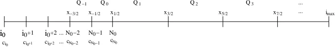
We use a finite volume scheme to approximate Equation (20). Let the mesh be defined byN0 =x1/2< x3/2 < ... < xN−1/2 =imax withIi = [xi−1/2, xi+1/2]

andhi =xi+1/2−xi−1/2, not necessarily uniform. We define the cell average

on the intervalIi as

Qk_i := 1

hi

Z xi+1/2

xi−1/2

c(x, tk)dx=

1

hi Z

Ii

c(x, tk)dx. (24)

The integral form of (20) on the interval [tk, tk+1] is given by

d dt

Z

Ii

c(x, t)dx=fi−1/2(c, c1∗, t)−fi+1/2(c, c∗1, t) (25)

with fi−1/2(c, c∗1, t) = c∗1(t)kon(xi−1/2)c(xi−1/2, t). By integration, we obtain

the time stepping scheme

Qk_i+1 =Qki −

∆t hi

(F_ik₊₁_/₂−F_ik₋₁_/₂) (26)

with

F_ik₋₁_/₂≈ 1

∆t

Z tk+1

tk

fi−1/2(c, c∗1, t)dt (27)

being an approximation to the average flux on the interval [tk, tk+1].

Choos-ingF_ik₋₁_/₂ =c1∗(tk)koni−1/2Qk_i₋₁ withkoni−1/2 :=kon(xi−1/2), we have the simple

upwind method

Qk_i+1=Qk_i −∆t

hi

c∗₁,k(k_oni+1/2Qk_i −k_oni−1/2Qk_i₋₁). (28)

This scheme is of first order. To increase the accuracy of the numerical simula-tions, we add a second order correction term and employ a Flux Limiter method on a non-uniform mesh [15, Chapter 6.17.1]. We have

Qk_i+1=Qk_i −∆t

hi

c∗₁,k(k_oni+1/2Qk_i −k_oni−1/2Qk_i₋₁)−∆t

hi( ˜

F_ik₊₁_/₂−F˜_ik₋₁_/₂), (29)

where we approximate the correction term by

˜ Fik−1/2=

c∗₁,k 2

hi−1−c

∗,k

1 k

i−1/2

on ∆t

kion−1/2

Qki −Qki−1 1

2(hi−1+hi)

Φ(λki−1) (30)

with

λki−1=

( _Qk

i−1−Q

k

i−2

Qk

i−Qki−1

, Qk

i 6=Qki−1

(10)

For Φ(λk

i) = 1, we obtain the Lax-Wendroff (LW) method which is a classical

second order scheme. However, it often leads to oscillations if sharp fronts are present in the solution.

As second choice we use the Van Leer (VL) Limiter given by

Φ(λ) =|λ|+λ 1 +|λ| =

(

0, λ <0

2|λ|

1+|λ|, λ >0

. (32)

Last, we will use a combination of Beam-Warming and Lax-Wendroff (BWLW) defined through

Φ(λ) =  



0, λ≤0

λ, 0≤λ≤1

1, 1≤λ

. (33)

2.2 Implementation of Boundary conditions

To advance the overall algorithm by one time step, we first compute ci0(tk+1)

and solve the finite ODE systemck_i+1fori= 1, .., N0. The computation ofQn1+1

in (26) requires the flux Fk

−1/2 which is outside the defined problem domain.

One approach would be to employ a special formula for the first cell and to compute the flux (27) by numerical integration. This in our case is not possible as c∗1,k+1 is necessary, but still unknown (we will discuss the exact algorithm

in Section 2.3). As alternative, we use a ghost cell approach as defined in [15]. The main idea is to make use of the solution of the ODE at time tn. As we

i0

i0 i0 i0

i 0

c ci 0 ci 0

N0 N0 N0

c_N0 c_N0 c_N0 +1 +2

x−3/2 x−1/2 x1/2 x3/2 x5/2 x7/2

Q

Q−1 Q0 Q1 2 Q3

+1 +2 ...

...

imax

... ...

−1 −2

−2 −1

Figure 1: Mesh interpretation for ghost cell approach

have a hyperbolic equation, all information is transported along the streamlines through the domain. We define x−1/2 := N0−1, x1/2 = N0 and define the

linear function

g(x) =cN0−1+ (x−N0+ 1) (cN0−cN0−1) (34)

forx∈[N0−1, N0]. We then define

Qk0:=

Z x1/2

x₋1/2

g(x)dx (35)

(11)

2.3 The algorithm

To obtainc∗₁,k, we need to compute the total polymerized mass Mk. In case of our ODE-PDE approximation, the total polymerized mass is given byMk =

Mk

ode+Mpdek with

M_odek =

N0

X

i=i0

ick_i, M_pdek = Z ∞

N0

xc(x, tk)dx.

Let now xi be the midpoint ofIi, i.e. xi = 1₂(xi−1/2+xi+1/2). As in [12], we

use the approximation

Mpde(tk) = N X

i=1

Z

Ii

xc(x, tk)dx≈ N X

i=1 xi

Z

Ii

c(x, tk)dx= N X

i=1

xihiQki.

The computational algorithm is thus given by

1. Givenc∗

1(tk), computeci0(tk+1).

2. Givenci0(tk), solve the finite ODE system forc

k+1

i ,i= 1, .., N0.

3. Givenck N0−1, c

k

N0, compute a ghost cell averageQ

k

0. (Analogously forQk−1, Qk

−2 in case of the flux limiter methods).

4. Solve the PDE using one of the methods defined in section 2.1 and obtain

c(xi, tk+1) fori=N0, .., N

5. Compute M(tk+1) and update c∗1(tk+1) with the mass balance equation

(23), i.e. c∗₁(tk+1) =c1(0)−Modek+1−Mpdek+1−c1(tk+1).

Remark 1. Time discretization.

In our numerical implementation, the ODE systen (38) fori≤N0is solved with

the forward Euler method. This scheme is explicit and of first order. To make use of the full higher order convergence that the Lax-Wendroff as well as Flux Limiter methods provide, it is necessary to also employ a second order scheme in time. The difficulty herein lies in the algorithm given above. A classical Runge-Kutta scheme can not be used, as it requires in step 2 the evaluation of

c∗1(tk+1)which is still unknown. A remedy is provided by the Adams-Bashforth

multi-step method, as it depends only on previous time steps. In our discussion below, we will keep however the backward Euler method. The CFL condition dictates a rather small time step for stability, such that the measured error is mainly spatial and convergence rates become clearly visible.

Remark 2. Properties of our scheme. By replacing (37) withc∗

(12)

c1(t), our scheme is conservative for the mass balance by construction. In case

of discretizing the PDE by the upwind scheme, we also have a positive method. On the uniform mesh, the Lax-Wendroff method as defined in (29) is consistent and of second order [15, Chapter 9].

3 Numerical Experiments

3.1 Description of numerical examples

3.1.1 Example 1

As a first example, we neglect the conformation step and choosec∗

1 =a ∈R,

use a constant polymerization ratekon ∈ Rand set kof f = 0. The equations

(10)-(13) then become

c∗1=a (36)

dci0

dt =k

N

on(c∗1)i0−konci0c

∗

1, (37)

dci

dt =c

∗

1kon(ci−1−ci), (38)

ci(0) = 0, i=i0, ...

A solution in closed form to this simplified model can be found.

Lemma 1. For c∗₁=a∈R_,_k_on _∈R_and_k_{of f} _{= 0}_{, we have}

ci0 =−

kN onai0−1

kon

e−konat₊k

N onai0−1

kon

, (39)

For i > i0, the polymer distribution is given by

ci+1(t) =ci(t)−(kona)i−i0

kNonai0

(i+ 1−i0)!

ti+1−i0_e−konat_. ₍₄₀₎

Having the exact solution provides the possibility to determine a discretiza-tion error for the distribudiscretiza-tioncof our method. However, we chose here to use a representative parameter set, for which the simulation of (40) becomes nu-merically unstable. When comparing the discretization error in the following section, we will therefore use a numerically computed distribution, obtained by (36), (39) and an explicit very accurate scheme for (38).

The inverse problem uses the total polymerized mass in the cost function, as this is measured in the experiments. In the following, we derive explicit solutions for the total polymerized mass to (36)-(38). Let therefore P = P_i_≥_i

(13)

add up equations (37) and (38) and use the telescoping sum

dP

dt =

dci0

dt +

X

i>i0

dci

dt

=kNon(c∗1)i0−konci0c

∗ 1+

X

i>i0

c∗1kon(ci−1−ci)

=kN_on(c∗₁)i0_.

WithP(0) = 0, we obtain

P(t) = Z t

0

k_onN(c∗₁)i0_dt₌_kN

onai0t. (41)

Similarly, we obtain the first moment (or total polymerized mass)M =P_i_≥_i₀ici

by multiplying equations (37) and (38) byiand summing overi

dM

dt =i0

dci0

dt +

X

i>i0

kdci dt

=i0konN(c∗1)i0−i0konci0c

∗ 1+

X

i>i0

c∗1kon((i−1)ci−1−ci+ci−1)

=i0konN(c∗1)i0+P c∗1kon.

SinceM(0) = 0, we find

M(t) = Z t

0

i0konN(c∗1)i0+konc∗1P ds=i0kNonai0t+

konkNonai0+1

2 t

2_. ₍₄₂₎

3.1.2 Example 2

In a second example, we again allow a conformation step and choose the poly-merization functionki

on to be linear ini, i.e.,

k_oni =k_on(1)+ik(2)_on

for some constants kon(1), kon(2) ∈ R. With this choice for koni , the setting is a

variation of the typical nucleation-aggregation model given by

dc1

dt =−k

+

Ic1+k−Ic∗1, (43)

dc∗1

dt =k

+

I c1−k−Ic

∗

1−i0kNon(c∗1)i0+i0kof fN ci0−c

∗ 1

X

i≥i0

koni ci, (44)

dci0

dt =k

N

on(c∗1)i0−kNof fci0−k

i0

onci0c

∗

1, (45)

dci

dt =c

∗

(14)

with initial conditions

ci(t= 0) =c∗1(t= 0) =ci0(t= 0) = 0, c1(t= 0) =c0. (47)

A solution in closed form cannot be found, but we derive an aggregated version of the model. We follow [19, Supplementary Data 1] and in an analogous manner as above obtain

dP

dt =k

N

on(c∗1)i0−kNof fci0 (48)

and

dM

dt =c

∗

1k(1)onP+c1∗kon(2)M+i0konN(c∗1)i0−i0kof fN ci0. (49)

Equations (43)-(45) and (48)-(49) form a (finite) system of ODEs which are eas-ily solved at a high precision using an explicit scheme. This numerical solution is then used in Section 3.2 to compute an error for the numerical approximation.

3.2 Numerical Results

We now present numerical results for the finite volume schemes applied to the two examples of the previous section. We make two choices for the mesh required in the discretization of the PDE. First, we use a simple uniform mesh defined as

xi=N0+i·h, i= 0, .., N

withh= imax−N0

N . Second, we use a progressive mesh that is defined such that

a ratio between the spatial step size and the corresponding mesh element is kept constant, i.e., ∆xi

xi =q <1. This results in the formula

xi =

1

1−qxi−1. (50)

Remark 3. The progressive mesh is a quasi uniform mesh in the sense that

∆xi−1

∆xi = 1−q= 1 +O(h). With this property, it can be shown that the upwind and Lax-Wendroff methods are consistent on the progressive mesh.

Based on the parameter estimation problem, where the cost-function uses the total polymerized mass M for the minimization process, we compute the relativeL2_[0_{, T}_{]-discretization error}_e

M as

eM =

kMh₋_M_k L2_[0_,T_]

(15)

withMh_{being the solution of the discretized problem. It should be emphasized}

here that the exact solution M corresponds to the infinite ODE setting, i.e.,

M =P_i_≥_i

0ici. We thus compare the numerical solution M

h _{(discretized by}

the ODE-PDE scheme) to the ODE solution. The obtained error is therefore always influenced by the quality of the continuous (PDE) approximation of the ODE system.

In case of Example 1, we also compute a relativeL2_{error for the distribution}_c

at the final timetN as

ec(tN) = P

i≥i0(˜ci(tN)−c

h₍_x₌_{i, t} N))2

1/2

P

i≥i0˜ci(tN)

21/2

. (51)

The approximation to the exact solution c is obtained, as described above, by solving (36), (39) and (38) with ∆tmax = 1e−3. The integer steps of

ch(x=i, tN) are obtained by linear interpolation between two grid pointsxk.

Again, we compare the solution of the ODE-PDE scheme to the (numerical) ODE solution. The observed error does not obey any convergence results known from the literature for an approximation of a PDE. However it will give a rough estimate of the convergence properties of our scheme.

To measure the computational efficiency of the schemes, we also include the computation times of each method. These are measured using the Matlab tic-toc command on an Intel Core i7 processor.

3.3 Example 1

We begin by investigating a uniform mesh for the PDE with N elements and compare the flux limiter methods. The parameters are chosen as

c0= 285·10−6, k_onN = 5.5079·103, kon= 2.1691·106,

imax= 3.2907·105,

i0= 3.

(16)

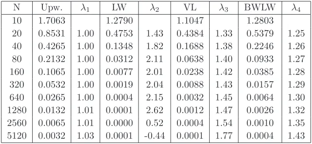
Table 1: Ex.1: ErroreM and convergence rates λi for the uniform mesh with

∆tmax=1e-3 andN0= 100.

N Upw. λ1 LW λ2 VL λ3 BWLW λ4

10 1.7063 1.2790 1.1047 1.2803

20 0.8531 1.00 0.4753 1.43 0.4384 1.33 0.5379 1.25

40 0.4265 1.00 0.1348 1.82 0.1688 1.38 0.2246 1.26

80 0.2132 1.00 0.0312 2.11 0.0638 1.40 0.0933 1.27

160 0.1065 1.00 0.0077 2.01 0.0238 1.42 0.0385 1.28 320 0.0532 1.00 0.0019 2.04 0.0088 1.43 0.0157 1.29 640 0.0265 1.00 0.0004 2.15 0.0032 1.45 0.0064 1.30 1280 0.0132 1.01 0.0001 2.62 0.0012 1.47 0.0026 1.32 2560 0.0065 1.01 0.0000 0.52 0.0004 1.54 0.0010 1.35 5120 0.0032 1.03 0.0001 -0.44 0.0001 1.77 0.0004 1.43

rather coarse spatial mesh) mainly a spatial error. We compute the simulations up to T = 40h. The discretization erroreM is found in Table 1 together with

the corresponding convergence rates. These are computed in the usual way as

λki =

log(eM(Nk)/eM(Nk−1))

log(Nk/Nk−1)

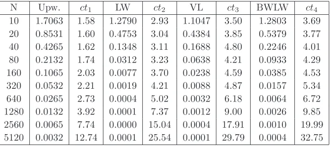
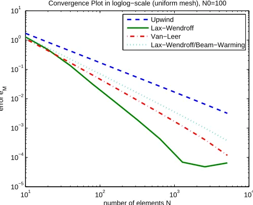
indicating the slope of the error curves in Figure 2. The computation times of each method with corresponding discretization error are presented in Table 2 and the polymer distributions are given in Figure 4.

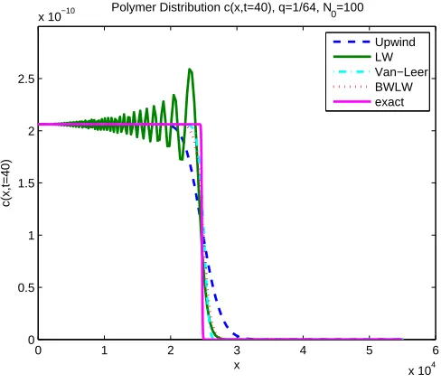
The simple upwind method converges with a rate of 1, while the Lax-Wendroff method converges with a rate of 2. The Flux-Limiter method rates are between 1 and 2 with the Van-Leer Limiter exhibiting a somewhat better convergence. The uniform mesh does not take the high concentration of smaller polymer sizes into account, but gives each spatial interval equal importance. The exact polymer distribution ci to Example 1 contains a sharp front. It is

thus expected and confirmed in Figure 4 that this feature will not be captured properly. The upwind method on a uniform grid smooths out the sharp front. While the Lax-Wendroff method converges the fastest forM, it leads to large oscillations for the distribution ci. The flux limiter methods avoid oscillations

and approximate the sharp front better than the upwind method. On the other hand, they have a slightly larger erroreM than Lax-Wendroff.

The first experiment for the progressive mesh keeps the ratioqfixed and changes

N0. The error does not change significantly. Due to the constant inflow of

conformers and as seen in Figure 3, the distributionci is constant for smaller

(17)

Table 2: Ex.1: Error eM for the uniform mesh and computation time cti,

∆tmax=1e-3,N0= 100

N Upw. ct1 LW ct2 VL ct3 BWLW ct4

10 1.7063 1.58 1.2790 2.93 1.1047 3.50 1.2803 3.69

20 0.8531 1.60 0.4753 3.04 0.4384 3.85 0.5379 3.77

40 0.4265 1.62 0.1348 3.11 0.1688 4.80 0.2246 4.01

80 0.2132 1.74 0.0312 3.23 0.0638 4.21 0.0933 4.29

160 0.1065 2.03 0.0077 3.70 0.0238 4.59 0.0385 4.53

320 0.0532 2.21 0.0019 4.21 0.0088 4.87 0.0157 5.34

640 0.0265 2.73 0.0004 5.02 0.0032 6.18 0.0064 6.72

1280 0.0132 3.92 0.0001 7.37 0.0012 9.00 0.0026 9.85

2560 0.0065 7.74 0.0000 15.04 0.0004 17.91 0.0010 19.99 5120 0.0032 12.74 0.0001 25.54 0.0001 29.79 0.0004 32.75

important. In the following simulations, we setN0= 100.

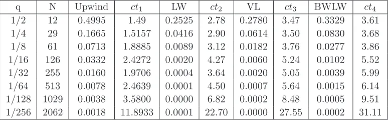
The second experiment for the progressive mesh focuses on the convergence of the error in q (or in the corresponding number of elements N). All meth-ods converge satisfactorily (Table 4 and 5 and Figure 3). In terms of the error

eM, the Lax-Wendroff method is best but again exhibits oscillations in the

dis-tribution c. In Figure 6, we present the relative error erel(t) = |M

h₍_t₎₋_M₍_t₎_|

|M| .

At the beginning, all methods have a large relative error. The model uses an instantaneous inflow of conformers which could be compared to a Dirac-delta function. Since all methods start with solving (38) up toi =N0, this peak is

the same for all cases. Fort≥1, the relative error is about constant and thus the approximationMh _{is found in a fan-shaped environment around}_M_{. It is}

clearly shown that Lax-Wendroff gives the best approximation toM, while the upwind method performs the worst.

Comparing the two meshes, the error using the progressive mesh is smaller than that using the uniform mesh. In conclusion, a choice for practical simulations would be a flux limiter method to avoid the oscillations in the approximation ofci in combination with a progressive mesh to make use of the smaller error.

3.4 Example 2

In the second numerical example, we approximate (43)-(46) using (16)-(20). The polymerization function is chosen as ki

on =k1on+ikon2 for the ODE, and

askon(x) =k1on+xkon2 in the continuous case. We use the following parameter

(18)

Table 3: Ex.1: ErroreM for the progressive mesh with ∆tmax= 10−3

q N0 N BWLW Upwind LW VL

0.10 10 97 0.0554 0.00549 0.0126 0.0199

0.10 100 77 0.0554 0.00549 0.0127 0.0199

0.10 1000 55 0.0553 0.00549 0.0127 0.0199

0.01 10 1009 0.0049 0.00005 0.0003 0.0008

0.01 100 803 0.0049 0.00003 0.0003 0.0008

0.01 1000 577 0.0049 0.00002 0.0003 0.0008

Table 4: Ex.1: ErroreM and convergence ratesλi for the progressive mesh with

∆tmax= 10−3 andN0= 100

q N Upwind λ1 LW λ2 VL λ3 BWLW λ4

1/2 12 0.4995 0.2525 0.2780 0.3329

1/4 29 0.1665 1.2451 0.0416 2.04 0.0614 1.71 0.0830 1.57

1/8 61 0.0713 1.1409 0.0089 2.08 0.0182 1.63 0.0277 1.48

1/16 126 0.0332 1.0536 0.0020 2.04 0.0060 1.53 0.0102 1.38

1/32 255 0.0160 1.0357 0.0004 2.17 0.0020 1.53 0.0039 1.36

1/64 513 0.0078 1.0266 0.0001 2.91 0.0007 1.56 0.0015 1.37

1/128 1029 0.0038 1.0312 0.0000 0.34 0.0002 1.76 0.0005 1.44 1/256 2062 0.0018 1.0413 0.0001 -0.86 0.0000 3.00 0.0002 1.75

Table 5: Ex.1: Error eM and computation time cti for the progressive mesh

with ∆tmax= 10−3 andN0= 100

q N Upwind ct1 LW ct2 VL ct3 BWLW ct4

1/2 12 0.4995 1.49 0.2525 2.78 0.2780 3.47 0.3329 3.61

1/4 29 0.1665 1.5157 0.0416 2.90 0.0614 3.50 0.0830 3.68

1/8 61 0.0713 1.8885 0.0089 3.12 0.0182 3.76 0.0277 3.86

1/16 126 0.0332 2.4272 0.0020 4.27 0.0060 5.24 0.0102 5.52

1/32 255 0.0160 1.9706 0.0004 3.64 0.0020 5.05 0.0039 5.99

1/64 513 0.0078 2.4639 0.0001 4.50 0.0007 5.64 0.0015 6.14

1/128 1029 0.0038 3.5800 0.0000 6.82 0.0002 8.48 0.0005 9.51

(19)

Figure 2: Example 1: Convergence plots for erroreM (uniform mesh)

101 102 103 104 10−5

10−4 10−3 10−2 10−1 100 101

Convergence Plot in loglog−scale (uniform mesh), N0=100

number of elements N

error e

M

Upwind Lax−Wendroff Van−Leer

Lax−Wendroff/Beam−Warming

Figure 3: Example 1: Convergence plots for erroreM (progressive mesh)

101 102 103 104 10−5

10−4 10−3 10−2 10−1 100

Convergence Plot in loglog−scale (progressive mesh), N0=100

error e

M

(20)

Figure 4: Example 1: Polymer Distribution (uniform mesh)

0 1 2 3 4 5 6

x 104 0

0.5 1 1.5 2 2.5

x 10−10

x

c(x,t=40)

Polymer Distribution c(x,t=40), N=640, N 0=100

Upwind LW Van−Leer BWLW exact

Figure 5: Example 1: Polymer Distribution (progressive mesh)

0 1 2 3 4 5 6

x 104 0

0.5 1 1.5 2 2.5

x 10−10

x

c(x,t=40)

Polymer Distribution c(x,t=40), q=1/64, N 0=100

(21)

Figure 6: Example 1: Development of errorerel in time (progressive mesh) for

q=1/32,N0= 100 and ∆tmax= 10−3

0 5 10 15 20 25 30 35 40 0

0.01 0.02 0.03 0.04 0.05 0.06 0.07 0.08 0.09

t

error e

rel

Development of relative error in time

upwind LW VL BWLW

Table 6: Ex.1: Errorec and convergence rates λi for the uniform mesh with

∆tmax= 10−3 andN0= 100

N Upwind λ1 LW λ2 VL λ3 BWLW λ4

80 3.11e-01 2.35e-01 2.52e-01 2.59e-01

(22)

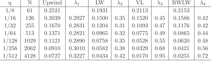
Table 7: Ex.1: Errorec and convergence ratesλi for the progressive mesh with

∆tmax= 10−3 andN0= 100

1/8 61 0.2521 0.1931 0.2113 0.2153

1/16 126 0.2039 0.2927 0.1500 0.35 0.1520 0.45 0.1586 0.42

1/32 255 0.1670 0.2831 0.1204 0.31 0.1093 0.47 0.1176 0.42

1/64 513 0.1371 0.2821 0.0965 0.32 0.0775 0.49 0.0865 0.44

1/128 1029 0.1121 0.2890 0.0758 0.35 0.0528 0.55 0.0620 0.48 1/256 2062 0.0910 0.3010 0.0582 0.38 0.0329 0.68 0.0421 0.56 1/512 4128 0.0727 0.3227 0.0434 0.42 0.0170 0.95 0.0255 0.72

c0= 285·10−6, k_I+= 5.7428·10−1, k−_I = 1·10−2_, kN_on= 5.5079·103_, k1_on= 8.2766103,

k2_on= 6.5916·103, imax= 3.2907·105,

i0= 3.

The simulated curve for the total polymerized mass has a typical shape (Figure 11) for the polymerization-aggregation model. After having a lag-phase at the beginning where the conforming step takes place, it grows steeply (polymeriza-tion) and damps out in the end when all monomers are bound to a polymer.

We again discuss the convergence of the different suggested schemes in terms of the total polymerized massM. This example does not permit an exact solution. We solve the (finite) system of ODEs (43)-(45) and (48)-(49) numerically, which gives a good approximation ˜M to the exact solution. The approximation error is then computed as

eM˜ =

kM˜ −MhkL2_[0_,T_]

kM˜kL2_[0_,T_]

(52)

We define a maximum time step size to solve the ODE system for ˜M, while the minimum time step size is determined through the CFL condition. In the follow-ing numerical computations, we use ∆tmax= 10−4. For the uniform mesh, we

(23)

Table 8: Ex.2: Errore_M˜ and convergence rates λi for the uniform mesh with

∆tmax= 10−3 andN0= 100

10 0.5400 0.5234 0.4761 0.5234

20 0.5065 0.09 0.4808 0.12 0.3944 0.27 0.4808 0.12

40 0.4642 0.13 0.4277 0.17 0.2859 0.46 0.4277 0.17

80 0.4130 0.17 0.3649 0.23 0.1796 0.67 0.3650 0.23

160 0.3537 0.22 0.2948 0.31 0.1071 0.75 0.2948 0.31

320 0.2882 0.30 0.2213 0.41 0.0651 0.72 0.2214 0.41

640 0.2207 0.38 0.1504 0.56 0.0389 0.74 0.1505 0.56

1280 0.1568 0.49 0.0888 0.76 0.0209 0.90 0.0891 0.76 2560 0.1023 0.62 0.0432 1.04 0.0094 1.15 0.0439 1.02 5120 0.0615 0.74 0.0164 1.40 0.0034 1.46 0.0173 1.35 10240 0.0345 0.83 0.0044 1.89 0.0010 1.82 0.0057 1.60

computation times for the four different methods using the uniform mesh with

N0= 100 andN0= 500 are given in Tables 8 - 11. For the progressive mesh, the

errorse_M˜ and convergence rate are given in Tables 12 - 16. We distinguish

be-tween ∆tmax= 0.5·10−3and ∆tmax= 10−3, as well asN0= 100 andN0= 500.

For the uniform mesh and N0 = 100 and N0 = 500, the numerical method

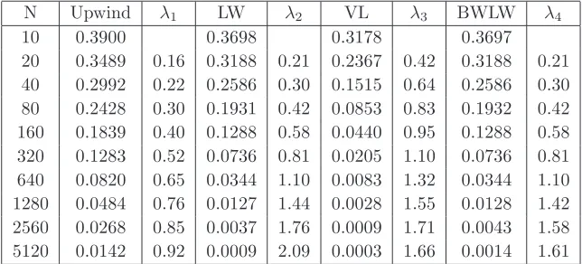
has not reached the asymptotic range yet for N, as the convergence rates are still changing. A convergence rate of 1 for the upwind method and 2 for the LW method are likely. We stopped the computations at this point and did not further investigate the convergence rates, as the computation times in combi-nation with the size of the error had already reached an impractical size for our application. It should be noted that the errore_M˜ is smaller forN0 = 500

throughout all methods and mesh sizes. This confirms the theory; the longer we use the actual ODE model for smaller polymers, the better is the approximation.

In case of the progressive mesh, the numerical scheme ceases to converge at a certain mesh size. To explain this, we first lowered the maximum time step size, to exclude that the error is caused by the temporal approximation. Having a smaller time step however gives an error in roughly the same range as be-fore. We may conclude that the stagnating error is not caused by the temporal approximation. Recall that the PDE is only an approximation to the infinite ODE system, but the error e_M˜ is computed with respect to the (numerical)

ODE solution. IncreasingN0 to 500 shows a smaller error and the stagnated

(24)

ob-Table 9: Ex.2: Errore_M˜ and computation timecti for the uniform mesh with

∆tmax= 10−3 andN0= 100

N Upwind ct1 LW ct2 VL ct3 BWLW ct4

10 0.5400 0.61 0.5234 0.90 0.4761 1.14 0.5234 1.19

20 0.5065 0.62 0.4808 0.90 0.3944 1.16 0.4808 1.22

40 0.4642 0.62 0.4277 0.93 0.2859 1.18 0.4277 1.23

80 0.4130 0.66 0.3649 1.08 0.1796 1.24 0.3650 1.30

160 0.3537 0.76 0.2948 1.44 0.1071 1.63 0.2948 1.71

320 0.2882 0.89 0.2213 1.78 0.0651 2.06 0.2214 1.76

640 0.2207 1.10 0.1504 1.82 0.0389 2.42 0.1505 2.63

1280 0.1568 2.13 0.0888 4.11 0.0209 5.44 0.0891 5.48

2560 0.1023 8.10 0.0432 16.21 0.0094 21.10 0.0439 21.34

5120 0.0615 24.07 0.0164 50.11 0.0034 62.94 0.0173 73.25

10240 0.0345 104.97 0.0044 198.91 0.0010 234.69 0.0057 267.99

Table 10: Ex.2: Errore_M˜ and convergence ratesλi for the uniform mesh with

∆tmax= 10−3 andN0= 500

10 0.3900 0.3698 0.3178 0.3697

20 0.3489 0.16 0.3188 0.21 0.2367 0.42 0.3188 0.21

40 0.2992 0.22 0.2586 0.30 0.1515 0.64 0.2586 0.30

80 0.2428 0.30 0.1931 0.42 0.0853 0.83 0.1932 0.42

(25)

Table 11: Ex.2: Errore_M˜ and computation timescti for the uniform mesh with

∆tmax= 10−3 andN0= 500

N Upwind ct1 LW ct2 VL ct3 BWLW ct4

10 0.3900 0.77 0.3698 1.09 0.3178 1.31 0.3697 1.35

20 0.3489 0.78 0.3188 1.07 0.2367 1.34 0.3188 1.42

40 0.2992 0.79 0.2586 1.13 0.1515 1.37 0.2586 1.43

80 0.2428 0.81 0.1931 1.16 0.0853 1.44 0.1932 1.49

160 0.1839 0.88 0.1288 1.29 0.0440 1.55 0.1288 1.62

320 0.1283 0.94 0.0736 1.43 0.0205 2.02 0.0736 1.90

640 0.0820 1.33 0.0344 1.96 0.0083 2.49 0.0344 2.62

1280 0.0484 2.64 0.0127 4.53 0.0028 6.08 0.0128 7.45

2560 0.0268 9.15 0.0037 17.39 0.0009 20.89 0.0043 22.81 5120 0.0142 27.48 0.0009 52.64 0.0003 64.11 0.0014 72.69

Table 12: Ex.2: Error e_M˜ and convergence rates λi for the progressive mesh

1/2 12 0.2857 0.2018 0.1253 0.1990

1/4 29 0.1480 0.75 0.0475 1.64 0.0159 2.34 0.0488 1.59

1/8 61 0.0726 0.96 0.0102 2.07 0.0023 2.58 0.0114 1.95

1/16 126 0.0354 0.99 0.0018 2.38 0.0002 3.24 0.0027 1.99

1/32 255 0.0172 1.02 0.0003 2.54 0.0004 -0.73 0.0005 2.48

1/64 513 0.0083 1.04 0.0007 -1.11 0.0007 -0.82 0.0004 0.12

1/128 1029 0.0039 1.09 0.0008 -0.21 0.0009 -0.39 0.0008 -0.83 1/256 2062 0.0017 1.19 0.0008 -0.05 0.0010 -0.28 0.0008 -0.05

tained a converged solution for the chosenN0 for which the error to the ODE

model can only be diminished by choosing a larger N0 or a better continuous

approximation to the ODE system (e.g., a second order PDE).

The goal of our study was to find an efficient scheme for the nucleation step in terms of accuracy and computation time. Fixing an acceptable computa-tion time of 1.5s, for example, and interpreting ˜M as good approximation to the exact solution, we can make several conclusions from Tables 13 and 16. ForN0= 100 and for the allowed upper temporal bound, the Upwind method

achieves a minimal error of 4·10−3_{, while LW and VL fall below an error of}

3·10−4_{. The VL method performs best with an error of 0.02% in 1.38s. A}

similar outcome is observed for N0 = 500 in Table 16. Again for a maximal

(26)

Table 13: Ex.2: Errore_M˜ and computational timesctifor the progressive mesh

1/2 12 0.2857 0.63 0.2018 0.93 0.1253 1.21 0.1990 1.19

1/4 29 0.1480 0.62 0.0475 0.93 0.0159 1.19 0.0488 1.23

1/8 61 0.0726 0.64 0.0102 0.96 0.0023 1.22 0.0114 1.29

1/16 126 0.0354 0.71 0.0018 1.10 0.0002 1.38 0.0027 1.42

1/32 255 0.0172 0.76 0.0003 1.25 0.0004 1.51 0.0005 1.60

1/64 513 0.0083 0.97 0.0007 1.74 0.0007 1.91 0.0004 2.00

1/128 1029 0.0039 1.16 0.0008 2.14 0.0009 2.82 0.0008 3.11 1/256 2062 0.0017 2.41 0.0008 3.71 0.0010 4.66 0.0008 4.99

Table 14: Ex.2: Error e_M˜ and convergence rates λi for the progressive mesh

with ∆tmax= 0.5·10−3 andN0= 100

1/2 12 0.2857 0.2017 0.1252 0.1990

1/4 29 0.1480 0.75 0.0474 1.64 0.0157 2.35 0.0487 1.59

1/8 61 0.0726 0.96 0.0100 2.09 0.0022 2.67 0.0113 1.96

1/16 126 0.0354 0.99 0.0016 2.49 0.0001 4.41 0.0026 2.04

1/32 255 0.0172 1.02 0.0004 1.96 0.0005 -2.53 0.0003 2.98

1/64 513 0.0083 1.04 0.0008 -1.01 0.0008 -0.67 0.0006 -0.86 1/128 1029 0.0039 1.09 0.0010 -0.18 0.0011 -0.33 0.0010 -0.71 1/256 2062 0.0017 1.19 0.0010 -0.04 0.0012 -0.24 0.0010 -0.04

0.03% in 1.45s (with q=1/16), which is about 8x smaller than the corresponding Upwind error of 0.23% in 1.34s (with q=1/128).

(27)

Table 15: Ex.2: Error eM˜ and convergence rates λi for the progressive mesh

1/2 10 0.2022 0.1429 0.0901 0.1406

1/4 23 0.0992 0.85 0.0329 1.76 0.0119 2.43 0.0334 1.73

1/8 49 0.0474 0.98 0.0074 1.98 0.0018 2.50 0.0078 1.92

1/16 101 0.0228 1.01 0.0017 2.05 0.0003 2.45 0.0019 1.97

1/32 205 0.0110 1.03 0.0004 2.17 0.0001 1.32 0.0005 1.99

1/64 412 0.0053 1.06 0.0001 1.37 0.0001 -0.09 0.0001 1.61

1/128 827 0.0024 1.12 0.0002 -0.16 0.0001 -0.15 0.0001 0.21 1/256 1657 0.0010 1.26 0.0002 -0.09 0.0002 -0.14 0.0001 -0.18

Table 16: Ex.2: Errore_M˜ and computational timesctifor the progressive mesh

1/2 10 0.2022 0.82 0.1429 1.18 0.0901 1.42 0.1406 1.41

1/4 23 0.0992 0.81 0.0329 1.11 0.0119 1.38 0.0334 1.43

1/8 49 0.0474 0.81 0.0074 1.13 0.0018 1.43 0.0078 1.50

1/16 101 0.0228 0.88 0.0017 1.22 0.0003 1.47 0.0019 1.52

1/32 205 0.0110 0.88 0.0004 1.33 0.0001 1.67 0.0005 1.76

1/64 412 0.0053 1.06 0.0001 1.58 0.0001 2.00 0.0001 2.12

1/128 827 0.0024 1.34 0.0002 2.00 0.0001 2.62 0.0001 2.79

(28)

Figure 7: Example 2: Convergence plots of errore_M˜ (uniform mesh), ∆tmax=

10−3 _and_N 0= 100

101 102 103 104 105 10−4

10−3 10−2 10−1 100

Convergence Plot in loglog−scale (uniform mesh), N 0=100

error

Figure 8: Example 2: Convergence plots of errore_M˜ (uniform mesh), ∆tmax=

10−3 _and_N 0= 500

101 102 103 104 10−4

10−3 10−2 10−1 100

Convergence Plot in loglog−scale (uniform mesh), N₀=500

error

(29)

Figure 9: Example 2: Convergence plots of error e_M˜ (progressive mesh),

∆tmax= 10−3 andN0= 100

101 102 103 104 10−4

10−3 10−2 10−1 100

Convergence Plot in loglog−scale, N 0=100

error

Figure 10: Example 2: Convergence plots of error e_M˜ (progressive mesh),

∆tmax= 10−3 andN0= 500

101 102 103 104 10−4

10−3 10−2 10−1 100

Convergence Plot in loglog−scale, N₀=500

error

(30)

Figure 11: Example 2: Distribution of polymers att= 12

0 100 200 300 400 500 0

0.2 0.4 0.6 0.8 1 1.2 1.4 1.6x 10

−9

x

c(x,t=12)

Polymer Distribution c(x,t=12), q=1/32, N 0=100

Upwind LW Van−Leer BWLW

Conclusion

This article proposes a method to deal numerically with both small sizes, pre-dominant during early reaction phases for instance, and with very large aggre-gates. It is based on a mixed ODE-PDE approach, which keeps the original ODE system for small sizes and uses an approximate PDE, on a progressive grid, for larger sizes. Tested on simplified cases for which explicit solutions are available, the method proved to be accurate, especially when using a flux limiter method in combination with a progressive mesh.

For the PDE component, we used finite volume methods which were accu-rate for the simplified case we were investigating. The methods presented in this paper neglect the possibility of depolymerization. However, they could be applied equally, by defining the flux limiter method according to [15, Chapter 9.5]

Fi−1/2=koni−1/2Qi−1+kidep−1/2Qi+ ˜Fi−1/2 (53)

where ˜Fi−1/2 is defined in [15, Chapter 9.3.1, (9.19)].

(31)

and accurate method developed by T. Goudon, F. Lagouti`ere and L.M. Tine in [12] for the Lifshitz-Slyozov equation, even if derived on uniform meshes, can be adapted on a non-uniform mesh, and others like [10] are already written on non-uniform grids.

References

1. J.P. Bourgade and F. Filbet. Convergence of a finite volume scheme for coagulation-fragmentation equations. Math. Comp., 77(262):851–882, 2008.

2. J. A. Caizo, L. Desvillettes, and K. Fellner. Regularity and mass con-servation for discrete coagulation-fragmentation equations with diffu-sion. Annales de lInstitut Henri Poincare. Annales: Analyse Non Lin-eaire/Nonlinear Analysis, 27(2):639–654, 2010.

3. J. A. Carrillo and T. Goudon. A numerical study on large-time asymp-totics of the Lifshitz-Slyozov system.J. Sci. Comput., 20(1):69–113, 2004.

4. J.F. Collet, T. Goudon, F. Poupaud, and A. Vasseur. The Becker– D¨oring system and its Lifshitz–Slyozov limit. SIAM J. on Appl. Math., 62(5):1488–1500, 2002.

5. J.F. Collet and S. Hariz. A modified version of the Lifshitz-Slyozov model. Applied Mathematics Letters, 12:81–95, 1999.

6. P Deuflhard, W Huisinga, T Jahnke, and M Wulkow. Adaptive discrete Galerkin methods applied to the chemical master equation. Technology, 30(6):2990–3011, 2008.

7. M. Doumic, T. Goudon, and T. Lepoutre. Scaling limit of a discrete prion dynamics model. Comm. in Math. Sc., 7(4):839–865, 2009.

8. F. Filbet and P. Lauren¸cot. Numerical approximation of the Lifshitz-Slyozov-Wagner equation. SIAM J. Numer. Anal., 41(2):563–588 (elec-tronic), 2003.

9. F. Filbet and P. Lauren¸cot. Mass-conserving solutions and non-conservative approximation to the Smoluchowski coagulation equation. Arch. Math. (Basel), 83(6):558–567, 2004.

(32)

11. Francis Filbet. An asymptotically stable scheme for diffusive coagulation-fragmentation models. Commun. Math. Sci., 6(2):257–280, 2008.

12. T. Goudon, F. Lagouti`ere, and L.M. Tine. The Lifschitz-Slyozov equation with space-diffusion of monomers. Kinetic and Related Models, 5(2):325– 355, 06 2012.

13. J. Kumar, M. Peglow, G. Warnecke, S. Heinrich, and L. Mrl. Improved ac-curacy and convergence of discretized population balance for aggregation: The cell average technique. Chemical Engineering Science, 61(10):3327 – 3342, 2006.

14. Lauren¸cot, P., and S. Mischler. From the discrete to the continuous coagulation-fragmentation equations. Proc. Roy. Soc. Edinburgh Sect. A, 132(5):1219–1248, 2002.

15. Randall J. LeVeque. Finite Volume Methods for Hyperbolic Problems. Cambridge Texts in Applied Mathematics. Cambridge University Press, Cambridge, 2002.

16. J. Masel, V.A.A. Jansen, and M.A. Nowak. Quantifying the kinetic pa-rameters of prion replication. Biophysical Chemistry, 77(2-3):139 – 152, 1999.

17. F. Oosawa and S. Asakura. Thermodynamics of the Polymerization of Protein. Academic Press, 1975.

18. Oliver Penrose. Metastable states for the becker-dring cluster equations. Communications in Mathematical Physics, 124(4):515–541, 1989.

19. S. Prigent, A. Ballesta, F. Charles, N. Lenuzza, P. Gabriel, L.M. Tine, H. Rezaei, and M. Doumic. An efficient kinetic model for assemblies of amyloid fibrils and its application to polyglutamine aggregation. PLoS ONE, 7(11):e43273, 11 2012.

20. Suzanne S. Sindi and Tricia R. Serio. Prion dynamics and the quest for the genetic determinant in protein-only inheritance. Current Opinion in Microbiology, 12(6):623–630, 2009.