University of Windsor University of Windsor
Scholarship at UWindsor
Scholarship at UWindsor
Electronic Theses and Dissertations Theses, Dissertations, and Major Papers
7-17-1969
Drought in the St. Clair Region.
Drought in the St. Clair Region.
Ronald C. A. Johnson
University of Windsor
Follow this and additional works at: https://scholar.uwindsor.ca/etd
Recommended Citation Recommended Citation
Johnson, Ronald C. A., "Drought in the St. Clair Region." (1969). Electronic Theses and Dissertations. 6566.
https://scholar.uwindsor.ca/etd/6566
This online database contains the full-text of PhD dissertations and Masters’ theses of University of Windsor students from 1954 forward. These documents are made available for personal study and research purposes only, in accordance with the Canadian Copyright Act and the Creative Commons license—CC BY-NC-ND (Attribution, Non-Commercial, No Derivative Works). Under this license, works must always be attributed to the copyright holder (original author), cannot be used for any commercial purposes, and may not be altered. Any other use would require the permission of the copyright holder. Students may inquire about withdrawing their dissertation and/or thesis from this database. For additional inquiries, please contact the repository administrator via email
INFORMATION TO USERS
This manuscript has been reproduced from the microfilm master. UMI films the text directly from the original or copy submitted. Thus, some thesis and dissertation copies are in typewriter face, while others may be from any type of computer printer.
The quality of this reproduction is dependent upon the quality of the copy submitted. Broken or indistinct print, colored or poor quality illustrations and photographs, print bleedthrough, substandard margins, and improper alignment can adversely affect reproduction.
In the unlikely event that the author did not send UMI a complete manuscript and there are missing pages, these will be noted. Also, if unauthorized copyright material had to be removed, a note will indicate the deletion.
Oversize materials (e.g., maps, drawings, charts) are reproduced by sectioning the original, beginning at the upper left-hand comer and continuing from left to right in equal sections with small overlaps.
ProQuest Information and Learning
By
RONALD C. A. JOHNSON
A THESIS
Undertaken as partial fulfillment of requirements for the M. A. degree
at the University of Windsor
Windsor, Ontario
UMI Number:EC52749
®
UMI
UMI Microform EC52749
Copyright 2007 by ProQuest Information and Learning Company. All rights reserved. This microform edition is protected against
unauthorized copying under Title 17, United States Code.
ProQuest Information and Learning Company 789 East Eisenhower Parkway
P.O. Box 1346 Ann Arbor, Ml 48106-1346
ABSTRACT
The St. Clair Region, although situated in a productive and humid agricultural area, suffers from moisture deficiency during the growing season great enough to decrease crop yields. The fre quency and severity of such moisture deficiency is important to determine the loss to farmers because of reduced yields and if irrigation would be a practical solution.
Monthly water balances were computed for the 12 climatological stations within the Region based on available record and soil type. The results were then statistically analysed to determine how severe drought is within the area.
Farmers were interviewed to determine to what extent they per ceived the danger of drought, and their reaction to drought con ditions .
The results showed a north to south variation in both precipita tion and potential evapotranspiration. This factor combined with different types of soils resulted in large variations of moisture deficiency throughout the Region. Although the farmers recognized the danger of drought, their reaction was quite different depending upon type of farm and expected increased yields.
Supplemental irrigation would greatly increase crop yields in the Region. Whether irrigation would be practical depends upon the increased value of the crop compared to the cost of irrigation.
ii
Expressions of gratitude must be given to the following persons and agencies for their kind assistance:
M. E. Sanderson, Department of Geography, University of Windsor
I. Stebelsky, Department of Geography, University of Windsor
Rev. J. F. Callaghan, Department of Economics, University of Windsor
J. R. Mather, C. W. Thornthwaite Associates, Centerton, New Jersey,
J. M. Fulton and staff, Agricultural Research Station, Harrow, Ontario.
TABLE OF CONTENTS
Page
A B S T R A C T ... ii
ACKNOWLEDGMENT... iii
LIST OF T A B L E S ... v
LIST OF ILLUSTRATIONS... vi
Chapter I. INTRODUCTION... 1
Definitions of Drought Four Types of Drought Results of Irrigation in Humid Areas II. M E T H O D O L O G Y ... 8
Water Balance Soils III. ANALYSIS OF D A T A ... 23
Precipitation Potential Evapotranspiration Deficiency During the Growing Season Monthly Deficiency IV. PERCEPTION OF THE DROUGHT H A Z A R D ... 58
The Sample Area I Area II Summary V. C O N C L U S I O N S ... 70
APPENDIX A ... 72
APPENDIX B ... 75
BIBLIOGRAPHY ... 77
iv
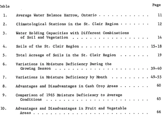
Tab le Page
1. Average Water Balance Harrow, Ontario ... II
2. Climatological Stations in the St. Clair Region ... 12
3. Water Holding Capacities with Different Combinations
of Soil and V e g e t a t i o n ... 14
4. Soils of the St. Clair R e g i o n ... 15-18
5. Total Acreage of Soils in the St. Clair R e g i o n ... 19
6. Variations in Moisture Deficiency During the
Growing Season ... 39-40
7. Variations in Moisture Deficiency by Month ... 49-55
8. Advantages and Disadvantages in Cash Crop A r e a s ... 60
9. Comparison of 1965 Moisture Deficiency to Average
C o n d i t i o n s ... 65
10. Advantages and Disadvantages in Fruit and Vegetable
LIST OF ILLUSTRATIONS
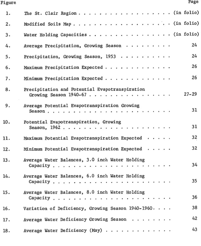
Figure Page
1. The St. Clair Region (in folio)
2. Modified Soils M a p ... . . (in folio)
3. Water Holding Capacities ... (in folio)
4. Average Precipitation, Growing Season ... 24
5. Precipitation, Growing Season, 1953 24
6. Maximum Precipitation Expected... 26
7. Minimum Precipitation Expected... 26
8. Precipitation and Potential Evapotranspiration
Growing Season 1940-67 ... 27-29
9. Average Potential Evapotranspiration Growing
Season... 31
10. Potential Evapotranspiration, Growing
Season, 1962 ... 31
11. Maximum Potential Evapotranspiration Expected ... 32
12. Minimum Potential Evapotranspiration Expected ... 32
13. Average Water Balances, 3.0 inch Water Holding
Capacity... 34
14. Average Water Balances, 6.0 inch Water Holding
Capacity... 35
15. Average Water Balances, 8.0 inch Water Holding
Capacity... 36
16. Variation of Deficiency, Growing Season 1940-1960. . . . 38
17. Average Water Deficiency Growing Season ... 42
18. Average Water Deficiency (May) ... 43
vi
19. Average Water Deficiency (June) ... 44
20. Average Water Deficiency (July) ... 45
21. Average Water Deficiency (August) ... 46
22. Average Water Deficiency (September) ... 47
23. Study Area 1 ... 62
CHAPTER 1
INTRODUCTION
The St. Clair Region, considered in the present study as Essex,
Kent and Lambton counties, lies in one of the most productive agri
cultural regions in Canada. Although possessing only 11.3 per cent
of the arable land in Ontario the St. Clair Region produces 15.7 per
cent of all principal field crops and 30.9 per cent of all fruits
and vegetables. The three county area dominates the Ontario pro
duction of soybeans (86%), shelled corn (45%), winter wheat (39%)
and barley (36%). The importance of the area is further emphasized
by the figures for the production of fruits and vegetables. Of the
total Ontario production of cantaloupes, tomatoes, pepper, beets, and
onions (market), Essex and Kent counties'*' produce 95, 72, 72, 57,
and 50 per cent respectively.
An area so dependent upon agricultural production will be greatly
affected economically by any climatic condition that reduces crop
yield. Experiments at Harrow^ have shown that seasonal rainfall is
almost always insufficient to allow maximum crop production.
The present study of moisture deficiency within the St. Clair
Region will analyse the frequency and severity of water shortages
within this area. Statistics were calculated with the aid of a
computer programme from the Thornthwaite Laboratory of Climatology,
New Jersey, which computes the monthly water balance} (Appendix A).
The monthly deficiencies will be analysed to show maximum and
1
minimum deficiencies expected, frequencies of varying degrees of defi
ciency and averages for both monthly and seasonal time periods.
The farmers perception of the danger of drought is also very
important in determining how they will react to the situation. By
use of a questionnaire an attempt was made to discover how great the
farmers felt the danger of water deficiency was to crop production
and their reaction to the situation.
Definitions of Drought
Drought is not an easily defined term. How severe must a water
shortage be before it is classed as a drought? How can the dividing
line between a moderate and severe drought be determined? These are
questions that have perplexed climatologists and agriculturalists for
many years.
Drought has most often been defined in terms of the amount of
rainfall below average conditions, or a period of consecutive days
without rainfall. The United States weather bureau considers drought
to exist whenever the rainfall for a period of 21 days or longer is
30 per cent of the average.3 The British Rainfall Organization defines
"absolute" drought as a period of 15 or more consecutive days without
rain, whereas a partial drought occurs after a period of 28 days with
rainfall averaging not more than one hundredth of an inch a day.
Russian meteorologists define drought as a period of ten days with a
total rainfall not exceeding a fifth of an inch.
Other attempts at a definition of drought have been less quan
3
relatively temporary departure of the climate from the normal or
average climate toward aridity."^" and " . . . a prolonged and abnormal
moisture deficiency."^ H. E. Thomas gives a more complicated definition:
drought (is) . . . a meteorological phenomenon which occurs during a period when precipitation is significantly less than the long term average and when this deficiency is great enough and continues long enough to affect mankind.
Drought has been defined in terms of its effects on vegetation.
One such definition by Barger and Thom considered drought to occur
after:
a specific period of time during which the total amount of rainfall recorded at a station is deficient to the extent that, more often than not, the yield falls below normal for the county in which the station is located.^
Tannehill more simply defines drought as " . . . a period of deficient
Q
rainfall that is seriously injurious to vegetation."
All of the above definitions have drawbacks. The definitions
offered by the United States weather bureau, the British Rainfall
Organization and the Russian weather bureau all define drought in terms
of rainfall alone. Drought obviously cannot be defined in this manner,
for such a definition would fail to take into consideration the amount
of water that was actually needed. For example, the effect of 15 days
without rainfall would be much greater if the soil were relatively dry
at the beginning of the 15 day period than if it had been saturated
with water.
The definitions of Palmer and Thomas, based on the events and
the end result of drought, fail to give a quantitative measure whereby
the intensity, duration or seriousness of a drought can be measured.
What actually constitutes a "prolonged and abnormal moisture deficiency"?
The definition of Burger and Thom is closer to a definition of
agricultural drought, but it too is unsatisfactory. A crude measure
of rainfall is not sufficient for accurate prediction of its effect
upon crop production. More precisely drought begins when the crop
cover can no longer draw upon the soil moisture rapidly enough to
replace that lost by evapotranspiration, with the result that the
actual evapotranspiration becomes less than the potential evapo
transpiration. This will not necessarily begin on the day that rain
ceases but will depend upon the potential evapotranspiration and level
of soil moisture.
Four Types of Drought
There are four basic types of drought. The first is permanent
drought. This occurs in the driest climates where there is always a
water deficit, vegetation is sparse and agriculture is only possible
by extensive irrigation. The second is seasonal drought which occurs
in areas with definite wet and dry seasons. Planting must be adjusted
so that the crop will grow through the wet season. Crops grown at other
times of the year must have irrigation. The third kind, contingent
drought, results from the fact that rainfall is irregular. Contin
gent drought is not limited to any special time period but is more
probable during the summer when potential evapotranspiration is high.
Contingent droughts are most commonly associated with subhumid and
humid climates and result in brief and irregular water shortages. A
fourth type of drought has been receiving increasingly greater attention.
5
rainfall is insufficient to restore the water lost by evaporation and
transpiration, with the result that the crop yield is greatly reduced.
When water is added by irrigation to overcome this deficiency the crop
yields can be significantly increased.
The question of invisible drought and its effect upon crop yield
is closely connected with two schools of thought that have developed
over the question of moisture stress on plants. The first, led by
Q
F. J. Viehmeyer, holds the view that water is rapidly available to
plants over the range from field capacity almost to the permanent
wilting point; that is, the actual evapotranspiration equals the
potential evapotranspiration until all available water is gone. The
second school of thought led by P. J. Kramer'*'® asserts that water
becomes progressively less available as the water content of the soil
decreases, with the result that the plants begin to suffer from water
deficits long before the water content reaches the permanent wilting
point. Thus Kramer's view is that the actual evapotranspiration equals
a decreasing fraction of the potential evapotranspiration as the water
level decreases.
The view held by Kramer is the generally accepted theory today.
G. Stanhi11 found, when studying eighty papers on soil moisture-crop
yield experiments, that over 80 per cent showed that plant growth was
affected by differences in available water: as soil moisture decreased,
plant growth was retarded. Invisible drought, therefore, seems to be
a definite factor in crop production.
Results of Irrigation in Humid Areas
The humid eastern part of North America, which includes Ontario
and eastern United States, generally has sufficient rainfall to support
the production of crops and pastures. Supplemental irrigation has been
used in the east to overcome the poor distribution of rainfall during
the growing season. The purpose of such irrigation has been to improve
the crop production, rather than enable the introduction of new crops as
has been the case in Western United States. Researchers have found that
supplemental irrigation results in higher yields and better quality
products by guarding against the effect of droughts. 12
Experiments at Athens, Georgia showed that supplemental irrigation
increased corn yields by 6 bushels per acre in years of nearly adequate
rainfall; in years of drought, however, the yields were increased by
T O
64 bushels per acre. Similarly E. E. Hartwig, P. Grissom, and W. A. Raney
found that supplemental irrigation of soybeans in the humid east increased
yields by 5 to 7 bushels per acre on sandy loam soil and 10 bushels per
acre on clay soil. Thus supplemental irrigation allowed maximum pro
duction by insuring that the plants were not deprived of water at any
7
REFERENCES
Agricultural statistics were obtained from Agricultural Statistics for Ontario, 1967, Ontario Department of Agriculture and Food (Toronto, 1968). Separate statistics are not available for Lambton County.
O
J. M. Fulton, "Soil Moisture for Crop Production," Canada Agri culture, (Winter, 1967), 1.
3
I. R. Tannehill, Drought; Its Causes and Effects (Princeton, 1947), p. 37.
^Wayne C. Palmer, Weekly Weather and Crop Bulletin, U. S. Weather Bureau, XIIV, No. la (January 10, 1957), 1.
^Wayne C. Palmer, "Meteorological Drought," U. S. Weather Bureau Research Paper No. 45. (February, 1965), 2.
% . E. Thomas, "General Summary of Effects of Drought in the South west," Geological _Survej professional ^Pajjer 372-H. (Washington: U. S.
Government Printing Office, 1963), 1.
^Gerald L. Barger and H. C. S. Thom, "A Method for Characterizing Drought Intensity in Iowa," Agronomy Journal, XLI (1949), 13-19.
^Tannehill, p. 39.
^F. J. Veihmeyer and A. H. Hendrickson, "Does Transpiration Decrease as.the Soil Moisture Decreases?" Transactions of the American Geophysical Union, XXXVI (1955), 425-428.
10p. J. Kramer, "The Role of Water in the Physiology of Plants," Advances in Agronomy, II, (1959), 51-70.
l^G. Stanhill, "The Effect of Differences in Soil Moisture Status on Plant Growth: A Review and Evaluation," Soil Science, LXXXIV (1957), 205-214.
^H. F. Rhoades and L. B. Nelson, "Growing 100-Bushel Corn with Irrigation," in Water, The Yearbook of Agriculture, ed. Alfred Stefferud (Washington, U. S. Department of Agriculture, 1955), p. 395.
^D. M. Whitt and C. H. M. Van Bavel "Irrigation of Tobacco, Peanuts and Soybeans," in Water, The Yearbook of Agriculture, ed. Algred
Stefferud (Washington, U. S. Department of Agriculture, 1955), p. 380.
METHODOLOGY
Water Balance
In choosing a method for calculating deficiency it was necessary
to find a system that could be used with the available data and one
that gave a fairly accurate measure of deficiency. Several such
methods are available. Two of the most common, those introduced by
Thornthwaite and Penman, employ similar approaches. Both methods are
based on computing potential evapotranspiration, computing actual evapo
transpiration as a function of potential evapotranspiration and soil
moisture, and a system of budgeting soil moisture.
Penman's method, although more theoretically sound than Thornthwaite'
has the difficulty of requiring parameters that are neither easily
measured nor easily available. The method chosen for this study, the
Thornthwaite water balance model, estimates monthly soil moisture and
deficiency with knowledge of only average temperature, precipitation and
type of soil. Such data are available for the St. Clair Region from
the Monthly Record published by the Department of Transport, and the
Ontario Soil Surveys published by the Ontario Department of Agriculture
and Food.
Many researchers have found a high correlation between measured
potential evapotranspiration and the Thornthwaite estimates. Smith-*-
in Trinidad found the Thornthwaite estimates to be as reliable as
9
Penman's. Sanderson^ at Windsor and Toronto found a very high correla
tion coefficient of r=.93 for measured and computed monthly estimates.
•3
Pelton, King and Tanner examined the use of air temperature to
derive potential evapotranspiration. Their criticisms are based on the
fact that potential evapotranspiration is dependent upon net radiation,
while air temperature is not a true measure of energy available for
evapotranspiration. Thornthwaite and Mather, in justifying the use of
mean temperature, found that mean temperature could serve as an index
of potential evapotranspiration because there is on a monthly basis a
fixed relationship between the net radiation used for heating and that
used for evaporation and that this ratio varies with temperature.^
It is known that as radiation (the energy needed for evaporation)
increases and decreases during the year, the temperature will vary
similarly, although there will be a lag effect. Pelton, King and Tanner
at Madison, Wisconsin found that the thermal lag is least when both
temperature and net radiation are maximum which occurs in July. This
lag effect will cause an underestimation of potential evapotranspiration
and deficiency in May and June, fairly accurate estimates in July, and
an overestimation in August and September.-*
Monthly figures were used rather than shorter time periods because
the accuracy of the method decreases with shorter periods of time. Pistor
found that the longer periods of measurement yielded more accurate
estimates of actual evapotranspiration. When correlating measured and
computed actual evapotranspiration on a one-day, five-day, ten-day and
monthly time periods in Harrow, he found a correlation coefficient of
r=.349, .784, .797, .939 respectively.^
Table 1 shows the average water balance for Harrow. The Thornthwaite
water balance uses potential evapotranspiration (P. E. line 3), defined
by Thornthwaite as the amount of water that would evaporate and trans
pire from a vegetated surface if available in optimum quantities at
all times. The crop, however, does not always have the moisture "avail
able to evaporate and transpire at the potential rate, but will use less
water as the soil moisture (line 7) decreases. The amount actually
used by the plant is the actual evapotranspiration (AE line 9) . The
difference between the potential and the actual evapotranspiration
represents the amount of water which was required by the plant cover,
but was not available, that is, the deficiency (line 10). This is the
"invisible drought," and the greater the deficiency during the growing
season, the greater the reduction in yield.
Twelve climatic stations are located within the St. Clair Region
with records varying from 9 to 28 years (see table 2). Although many
more stations would be desireable, their even spacing throughout the
region (figure 1 in folio)^ provides this area with one of the most
comprehensive coverages in Canada.
Soils
The use of the Thornthwaite water balance requires a knowledge of
the moisture holding capacity of the soil. For this, it is necessary
to know the root depths and the texture of the soil. These two factors
will give the water holding capacity for any combination of soil and
crop. Clay soil, for example, holds approximately 3.6 inches of water
R e p ro d u c e d w ith pe rmission of th e c o py ri g h t o w n e r. F u rth e r rep ro duc ti on p ro h ib it e d wi th o ut p e rm is s io n .
TABLE 1
AVERAGE WATER BALANCE HARROW ONTARIO
(Water Holding Capacity of 6.0 Inches)*
J F M A M J J A S 0 N D Year
X ]?** 25.6 26.4 33.5 45.9 57.4 68.3 72.7 71.3 63.8 52.8 39.7 28.8 48.9
Unadj PE 0 0 0 .04 .09 .13 .15 .14 . 11 .07 .02 0 29.01
PE 0 0 0 1.34 3.40 4.95 5.76 5.00 3.43 2.00 .49 0 26.37
P 2.26 2.16 2.32 2.68 2.68 3.09 2.52 2.61 2.25 2.21 2.11 2.12 P-PE 2.26 2.16 2.32 1.34 -.72 -1.86 -3.24 -2.39 -1.18 .21 1.62 2.12
Acc Pot WL -.72 -2.58 -5.82 -8.21 -9.39
ST 7.41 9.57 6.00 6.00 5.31 3.87 2.23 1.48 1.20 1.41 3.03 5.15 AST .85 0 0 0 -.69 -1.44 -1.64 -.75 -.28 .21 1.62 2.12
AE 0 0 0 1.34 3.37 4.53 4.16 3.36 2.53 2.00 .49 0 21.78
D 0 0 0 0 .03 .42 1.60 1.64 .90 0 0 0 4.59
S 0 0 5.89 1.34 0 0 0 0 0 0 0 0 7.23
RO 0 0 2.95 2.15 1.07 .54 .27 .14 .07 .03 .02 .01 7.23
* All values except T are in inches.
e p ro d u c e d w ith pe rmission of th e c o py rig h t o w n e r. F u rth e r re pr od uct ion p ro h ib ite d wi th o ut p e rm
TABLE 2
CLIMATOLOGICAL STATIONS IN THE ST. CLAIR REGION
Station
Years of
Record Station
Years of Record
Camlachie 9 Pelee Island 27
Chatham 28 Ridgetown 28
Forest+ 25 Sarnia 19
Harrow 28 Wallaceburg+ 22
Leamington 28 Windsor 27
Oil Springs*+ 13 Woodslee 21
13
Q
available to the crop when the soil is at field capacity.
The Laboratory of Climatology in Centerton, New Jersey has grouped
the number of soil types into 5 major classes: fine sand, fine sandy
loam, silt loam, clay loam and clay, each having unique water holding
capacity (see table 3). For the purposes of this study the soils
of the St. Clair Region have also been grouped into the same five cate
gories, as shown in Table 4.
Soil surveys and maps of Essex, Kent and Lambton Counties were
obtained from the Ontario Department of Agriculture and the soils
shown were grouped into the above five texture categories on the basis
of the percentage of clay, silt or sand in each type of soil. Figure 2
(in folio) shows the five soil classes of the St. Clair Region.
Table 5 summarizes the percentages of the various soils in the
St. Clair Region by county. The most predominant type of soil is
clay (59.2%). The remaining soils are much less prevalent in the
area: fine sandy loam (15.1%), clay loam (8.8%), silt loam (6.3%),
fine sand (5.9%) and miscellaneous soils (4.6%). The miscellaneous
soils have not been included in the breakdown of water holding capacities
(see figure 3 in folio) because they are made up of various soils which
are hard to define e.g. bottomland, or are not fully developed soils
e.g. marsh.^ These soils appear in only small patches throughout the
region except for areas in southwest Essex County, Point Pelee,
Rondeau, and northeast Lambton County. In other areas they are
found mainly along rivers or poorly drained lowlands. Because of this
scattered nature, diversity of soil type and the relatively small
percentage the miscellaneous soils covering the area, they have been
omitted from the deficiency studies.
TABLE 3
WATER HOLDING CAPACITIES WITH DIFFERENT COMBINATIONS OF SOIL AND VEGETATION
Soil Type Available Water IN/FT
Root Zone FT
Applicable Soil Moisture Retention Table
IN
Shallow-Rooted Crops Fine Sand
(Spinach, Peas, 1.2
Beets, Carrots, Etc.)
1.67 2.0
Fine Sandy Loam 1.8 1.67 3.0
Silt Loam 2.4 2.08 5.0
Clay Loam 3.0 1.33 4.0
Clay 3.6 .83 3.0
Moderately Deep-Rooted Crops (Corn, Fine Sand 1.2
Tobacco, Cereal Grains)
2.50 3.0
Fine Sandy Loam 1.8 3.33 6.0
Silt Loam 2.4 3.33 8.0
Clay Loam 3.0 2.67 8.0
Clay 3.6 1.67 6.0
Deep-Rooted Crops (Alfalfa, Pastures Fine Sand 1.2
, Shrubs)
3.33 4.0
Fine Sandy Loam 1.8 3.33 6.0
Silt Loam 2.4 4.17 10.0
Clay Loam 3.0 3.33 10.0
Clay 3.6 2.22 8.0
Orchards
Fine Sand 1.2 5.00 6.0
Fine Sandy Loam 1.8 5.55 10.0
Silt Loam 2.4 5.00 12.0
Clay Loam 3.0 3.33 10.0
Clay 3.6 2.22 8.0
Closed Mature Forest
Fine Sand 1.2 8.33 10.0
Fine Sandy Loam 1.8 6.66 12.0
Silt Loam 2.4 6.66 16.0
Clay Loam 3.0 5.33 16.0
Clay 3.6 3.90 14.0
15
TABLE 4
SOILS OF THE ST. CLAIR REGION
County Name of Soil Acreage
Class (By Thornthwai te
Laboratory)
Per Cent of County
Total
Essex Brookston Clay Toledo Clay Clyde Clay Jeddo Clay Caistor Clay Perth Clay 250,000 17.500 2.500 3.500 13.500 9,000 Clay 65.8
Total Clay 301,000
Perth Clay Loam Castor Clay Loam Brookston Clay Loam Burford Loam Burford Loam-Shallow 8,000 2,500 30,000 3,700 5,300
Clay Loam 10.8
Total Clay Loam 49,500
Toledo Silt Loam Harrow Loam Farmington Loam Parkhill Loam Parkhill Loam
Red Sand Spot Phase
1,000 4.000 2.000 5.000
5.000
Silt Loam 3.7
Total Silt Loam 17,000
Tuscola Fine Sandy Loam Colwood Fine Sandy Loam Harrow Sandy Loam
Fox Sandy Loam Berrien Sandy Loam Caistor Sand Spot Phase Brookston Clay Sand
Spot Phase Wauseon Sandy Loam
6,000 7.000 3.500 5,300 16,000 1.500 18,000 3.000
Fine Sandy
Loam 13.1
Total Fine Sandy Loam 60,300
TABLE 4— Continued
Class (By Per Cent Thornthwaite of County County Name of Soil Acreage Laboratory) Total
Essex Granby Sand Berrien Sand Plainfield Sand Eastport Sand
1,000
8,000
1,700 2,500
Fine Sand 2.8
Total Fine Sand 13,200
Bottom Land 7,300
Marsh 7,000 Miscellaneous 3.5
Muck 1,700
Total Miscellaneous 16,000
Kent Haldimand Clay 2,000 Napanee Clay 5,000
Brookston Clay 177,000 Clay 32.0 Clyde Clay 35,000
Total Clay 189,000
Miami Clay Loam 44,000 Miami Clay Loam
(Gravelly Phase) 5,000
Canover Clay Loam 8,000 Clay Loam 17.6 Canover Loam 2,000
Thames Clay Loam 18,000 Brookston Clay Loam 31,000
Total Clay Loam 104,000 Haldimand Loam 16,000 Beverly Loam 10,000
Brookston Silt Loam 37,000 Silt Loam 14.0 Brookston Loam 10,000
Clyde Silt Loam 10,000
17
TABLE 4— Continued
County Name of Soil Acreage
Class (By Thornthwaite
Laboratory)
Per Cent of County
Total
Kent Fox Sandy Loam Fox Gravelly Loam Berrien Sandy Loam Beverly Fine Sandy Loam Brookston Sandy Loam Clyde Loam
Gilford Gravelly Loam Brady Gravelly Loam
Total Sandy Loam
Plainfield Sand Berrien Sand Granby Sand
Total Fine Sand
Muck
Bottom Land Eroded
Total Miscellaneous
Lambton Huron Clay Perth Clay Brookston Clay Caistor Clay Toledo Clay Clyde Clay Blackwell Clay
Brookston and Berrien Complex
Perth and Berrien Complex
Total Clay
Caistor and Berrien Mixture
Toledo Clay Loam
400 17.000 46.000 9.000 51.000 17.000 2.000 1,000 143 ,400 300 53 ,000 9,000 62,300 7;,000 700 400 8:,100
19 :,100 137.,300 308.,300 69,,100 300 1=,900 8,,600 4,,700 1,,700 559,,000 1,,900 1, 200
Fine Sandy
Loam 24.3
Fine Sand 10.5
Miscellaneous 1.3
Clay 77.1
Clay Loam 0.4
Total Clay Loam 3,100
TABLE 4— Continued
County Name of Soil Acreage
Class (By Thornthwai te
Laboratory)
Per cent of County
Total
Lambton Lambton Silt Loam Shashawandah Loam Gilford Loam
11,400 500
100
Silt Loam 1.6
Total Silt Loam 12,000
Colwood Fine Sandy Loam 15,300 Fox Sandy Loam 4,700 Brady Sandy Loam 7,800 Granby Sandy Loam 1,800 Berrien Sandy Loam 7,100
Guelph Loam 500
Brisbane Loam 13,600 Burford Loam 8,000 Brady and Brookston
Mixture 4,800
Fine Sandy
Loam 8.7
Total Sand Loam 63,600
Plainfield Sand 15,900
Brady Sand 10,700
Eastport Sand 2,400 Fine Sand 4.0
Berrien Sand 100
Total Sand 29,100
Muck 4,500
Peat 900
Marsh 16,500 Miscellaneous 7.9
Bottomland 35,900
R e p ro d u c e d w ith pe rmission of th e c o py ri g h t o w n e r. F u rth e r rep ro duc ti on p ro h ib it e d wi th o ut p e rm is s io n . TABLE 5
TOTAL ACREAGE OF SOILS IN THE ST. CLAIR REGION
County Clay Clay Loam Silt Loam
Fine Sandy Loam
Fine
Sand Miscellaneous Totals
Essex 301,000 49,500 17,000 60,300 13,200 16,000 457,000
Kent 189,000 104,000 83,000 143,400 62,300 8,100 589,800
Lamb ton 559,000 3,100 12,000 63,600 29,100 57,800 724,700
Total Acreage 1,049,000 156,100 112,000 267,300 104,600 81,900 1,770,900
Percent of each Soil Type in
the Region 59.2 8. 8 6.3 15.1 5.9 4.6 99.9
The clay soils are most prominent in Lambton and Essex counties,
covering 77% and 66% of the area respectively- In Lambton the clay
soils cover all the area except near Sarnia, the northeast section,
near Port Lambton, along the east county boundary and a narrow band
of sand loam stretching from Thedford to Wyoming. In Essex County
clay is predominant in the interior of the county with various other
soils along the shoreline. Large areas of non-clay soils can be found
around Leamington, Windsor and the area from east of Kingsville to west
of Harrow. In Kent County the only large area of clay is in the south
west section.
The various loam soils cover 30.2 per cent of the total area of
the St. Clair Region. Clay loam is insignificant in Lambton County
(0.4%). Large patches can be found around Windsor, Malden Township
and Kingsville in Essex County and near Ridgetown, along Highway No. 2
east of Chatham in Kent County. Only small amounts of silt loam can be
found in Essex and Lambton Counties, 3.7 and 1.6 per cent respectively,
with the concentrations being at Harrow, northwest of Leamington and
around Watford. Large areas of silt loam can be found in Kent County
especially south of Wallaceburg and south and east of Chatham. The
largest loam soil is the fine sandy loam, covering 15.1 per cent of
the region's acreage. This soil is found in patches throughout the
region.
A large concentration of sandy soils is found in northeast Kent
and southeast Lambton as well as along the shoreline of Lambton County
from Port Frank to Grand Bend. Small patches are also found near Harrow
21
In the present paper only one type of crop, with moderately deep
roots e.g. corn and wheat, has been analyzed. This has been done since
these crops are the most important in the area. Thus the maps and tables
that follow apply to moderately deep-rooted crops only. Additional maps
would be necessary to study drought in shallow-rooted crops, deep-rooted
crops or orchards.
For the climatic model what is required is not a map of soil types,
but water holding capacities. Although the region has been divided into
five basic soil types, for moderately deep-rooted crops, only three
different water holding capacities result, using the Laboratory of Climat
ology figures. The water holding capacity is the product of the available
water per foot of soil and the root zone. For example, fine sandy loam,
with much less available water per foot of soil than clay (1.8 and 3.6
inches respectively,), has the same water holding capacity as clay because
the root zone of fine sandy loam is much deeper (see Table 3).
In the St. Clair Region 74 per cent of the land has a water holding
capacity of 6.0 inches, 15 per cent 8.0 inches and 6 per cent 3.0 inches.^1
REFERENCES
■*"G. W. Smith, "The Determination of Soil Moisture Under a Permanent Grass Cover," Journal of Geophysical Research, LXIV (1959), 477-483.
E. Sanderson, "Observations of Potential Evapotranspiration at Windsor, "Publications in Climatology, VII (1954), 91-93.
W. L. Pelton, K. M i King and C. B. Tanner, "An Evaluation of the Thornthwaite and Mean Temperature Methods for Determining Potential Evapotranspiration," Agronomy Journal, LII (1960), 387-395.
^C. W. Thornthwaite and J. R. Mather, "The Water Balance," Publications in Climatology, VIII (1955), 1-86.
-*Pelton, King and Tanner, pp. 388-90.
^Pistor, A Climatological Approach to Irrigation Scheduling: A Comparison of Three Methods of Computing Water Use (University of Windsor, 1967), p. 43.
^Maps 1 to 3 (in folio) are of the same scale and serve the purpose of locating more exactly where the various soils and water holding capacities are by means of overlays.
O
C. W. Thornthwaite and J. R. Mather, "Instructions and Tables for Computing Potential Evapotranspiration and the Water Balance, "Publications in Climatology, X (1956), 244.
^Miscellaneous soils form only a minor part of the soils in the St. Clair Region. Although some of these soils are quite productive agriculturally, they vary greatly in water holding capacity, making it impractical to include them in the study.
CHAPTER III
ANALYSIS OF DATA
Precipitation
1 9
Figure 4 shows the average precipitation for the growing season
in the St. Clair Region. The average precipitation ranges from less
than 14.0 inches at Harrow and Camlachie, to over 16.0 inches at
Forest. When the map of average growing season precipitation is
compared to a specific year, vast differences can be seen. Whereas
Figure 4 shows a variation of only 2 inches in the area, Figure 5
depicting the 1953 precipitation indicates strong spatial variation.
Figure 5 shows a definite decrease in precipitation from north to
south, with pockets of high precipitation around Windsor and Pelee
Island. The 1953 figures show a very large variation in precipitation
of greater than 12 inches, with a low near Harrow of less than 8 inches
and a high near Camlachie and Forest of greater than 20 inches.
Drastic variations in precipitation can occur in a relatively small
and uniform area such as the St. Clair Region.
Of interest to farmers is the maximum and minimum precipitation
that can be expected in any given area, and the chances of such a
situation occuring. To find this the standard deviations of the 4 growing season precipitation for all the stations were found.
Figure 6 shows the maximum precipitation expected. This was
obtained by plotting two standard deviations above the mean, that is
23
e p ro d u c e d w ith pe rmission of th e c o py ri g h t o w n e r. F u rth e r rep rod uct ion p ro h ib it e d wi th o ut p e rm
AVERAGE PRECIPITATION
GROWING SEASON
,
ISOLINE INTERVAL 2 INCHES
METEOROLOGICAL STATION
PRECIPITATION - 1953
ISOLINE INTERVAL 2 INCHES
25
97.5 per cent of all years will have precipitation of less than that
shown in Figure 6. This represents the maximum rainfall that can be
expected for the area. Essex and Kent counties appear to be the
areas of lowest rainfall expected whereas relatively heavy precipita
tion may occur in the northeast section of Lambton County.
Figure 7 shows the lowest rainfall that can be expected in 97.5
per cent of the years. Relatively uniform conditions exist through
out the region for the minimum precipitation expected, except around
Wallaceburg. In one year in 50 the precipitation can be expected to
be only 8 inches during the growing season.
The yearly growing season precipitation and potential evapotrans
piration at the 12 climatological stations (obtained from the climatic
water balance computer programme) is shown in Figure 8. While there
is relative stability of potential evapotranspiration, there is a
great variability in the amount of moisture received each year with
a maximum of 24.7 inches at Forest in 1945 and a minimum of 6.0 inches
at Chatham in 1954. This amounts to a variation over the whole region
of 18.7 inches of precipitation for the period of study. A great
variation can also be found for any one station. Forest had the largest
variation with a high of 24.7 inches of precipitation in 1945 and a
low of 7.7 inches in 1963 for a difference of 17.0 inches. The highest
variation in precipitation in any one year occured in 1953 when a high
was recorded at Forest of 21.8 inches and a low at Harrow of 8.7 inches,
for a difference of 18.1 inches.
O nr q A 0 °f-cS *_> KJ w O
e p ro d u c e d w ith pe rmission of th e c o py ri g h t o w n e r. F u rth e r re pr od uct ion p ro h ib it e d wi th o ut p e rm
MAXIMUM PRECIPITATION
EXPECTED
j
ISOLINE INTERVAL 2 INCHES
METEOROLOGICAL STATION
20
MINIMUM PRECIPITATION
EXPECTED
jISOLINE INTERVAL 2 IN C H ES
Inch es In c h e s 27
PRECIPITATION AND POTENTIAL EVAPOTRANSPIRATION
GROWING SEASON
CAMLACHIE
28 -i
24
-2 0
-O
to tD(O
o
4- at♦ IDin
Y e a r
a
FOREST
28
2 4
20
-CD
<0 O
<r GO o10 <oo Y e a r
C
---* P re c ip ita tio n
* — - Potential Evapotranspiration
F ig u
1 9 4 0 -1 9 6 7
CHATHAM 28 24 20 16 12 8 4 0 o o co <o CNJ in GO *
Y e a r
b HARROW 28 24 20 o to CO o GO
* ©CO
Ye a r
d
8
R eproduced with permission of the copyright owner. Further reproduction prohibited w ithout permission.
19
In
c
h
e
s
PRECIPITATION AND POTENTIAL EVAPOTRANSPIRATION
GROWING SEASON 1 9 4 0 -1 9 6 7
LEAMINGTON
28
24
20
</> ©
JZ
a
c
o o
<0 ©©
© N
tn
Year
e
PELEE ISLAND
28
24
W \
20 © © o o © *■© © * Year 9
— P recip itation
—* Potential Evapotranspiration
OIL SPRINGS
28 24 20 16 12 8 4 O o o © *© © * CVJ10
Year f RIDGETOWN 28 24 A
20
-o © CVJ
© ©© ©o *•© ©©
Year
h
19
6
In c h e s In c h e s 29
PRECIPITATION AND POTENTIAL EVAPOTRANSPIRATION
GROWING SEASON 1 9 4 0 -1 9 6 7
SARNIA WALLACEBURG
28
24
20
16
12 -
8 -
4 -
0
CO
o
“ T ”
CO
w o Y ea r
o (0 O) rr (0 a <D CO 0) 28
24 J
20 4
o co to
o
<5* CO CMW if
Y e a r
j
WINDSOR WOODSLEE
28
2 4 J
20 ^
CO
CO CO
o <r
■c COc* inCM COin COo
Y e a r
k 28 24 20 16 12 8
4 H
o 0) 'J-o
•'*> p -\ S' /'
/ \ t w I » i \ j* jr
* * \ I*' *' \
00 ’S' C) CM tn O CO <n
Y e a r
m
o
CO CO
o
P re c ip itatio n
Potential Evapotranspiration
Figure .8— C o n tinued
R eproduced with permission of the copyright owner. Further reproduction prohibited without permission.
19
68
,9
6
Potential Evapotranspiration
The potential evapotranspiration, the heat factor in the water
balance, appears to be much more uniform. Figure 9 indicates an
increase in the average potential evapotranspiration from north to
south of only about one inch for the five month growing season. In
1962, the year with the most variation in potential evapotranspiration
(Figure 10), the maximum difference was two inches. Figures 11 and
12 showing plus and minus two standard deviations again show a similar
pattern, but with larger variations, 4.2 inches for plus two standard
deviations and 2.2 inches for minus two standard deviations. In the
southern part of Essex County in 1 year in 50 the potential evapotrans
piration can be 24 inches, but in 1 year in 50 it can be less than 19
inches.
A maximum of 25.1 inches of potential evapotranspiration occured
at Harrow in 1944 and minimum of 19.0 inches at Sarnia and Oil City
in 1956 and 1958 respectively for a difference of 6.1 inches of
potential evapotranspiration. For one station the greatest variation
occured at Harrow where a high of 25.1 inches was recorded in 1944 and
a low of 20.0 inches in 1957 and 1958 for a difference of 5.1 inches,
a variation of 25 per cent. The year with the greatest variation was
1962 when Pelee Island recorded 23.7 inches of potential evapotranspira
tion and Forest 20.2 inches for a difference of 3.5 inches.
Deficiency During the Growing Season
To arrive at a quantitative measure of drought intensity and fre
R e p ro d u c e d w ith pe rmission of th e c o py ri g h t o w n e r. F u rth e r rep ro duc ti on p ro h ib it e d wi th o ut p e rm is s io n .
AVERAGE POTENTIAL
EVAPOTRANSPIRATION
GROWING SEASON
ISOLINE INTERVAL I INCH
• METEOROLOGICAL STATION
Figure 9
POTENTIAL EVAPOTRANSPIRATION
1962
ISOLINE INTERVAL I INCH
METEOROLOGICAL STATION
U>
e p ro d u c e d w ith pe rmission of th e c o py ri g h t o w n e r. F u rth e r rep ro duc ti on p ro h ib it e d wi th o ut p e rm
MAXIMUM
POTENTIAL
EVAPOTRANSPIRATION
EXPECTED
ISOLINE INTERVAL I INCH
• METEOROLOGICAL STATION
MINIMUM
POTENTIAL
EVAPOTRANSPIRATION
EXPECTED
ISOLINE INTERVAL I INCH
33
several years. Computerized water balances were run using water holding
capacities of 3, 6, and 8 inches for each of the 12 stations within the
Region, for the period of time available from 9 to 28 years.
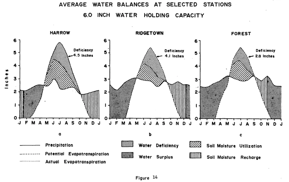
Three stations were selected for purposes of comparison: Harrow,
which has the greatest deficiency; Forest, which has the least deficiency;
and Ridgetown, which has a deficiency between the two extremes. Figures
13 to 15 show the average monthly precipitation, potential evapotranspira
tion and monthly deficiency at the three stations using 3, 6, and 8 inch
water holding capacities.
All three stations have similar graphs. The potential evapotrans
piration is 0 in the winter months but begins to rise in the early spring,
reaching a peak in July of between 5.0 and 6.0 inches. It then falls
rapidly in autumn until 0 potential evapotranspiration is again reached
in December. The precipitation is more evenly distributed throughout
the year with a monthly variation at Forest, Ridgetown and Harrow of
only 1.0, 1.1, and 1.0 inches respectively.
Although rainfall exceeds potential evapotranspiration on an annual
basis at all three stations, during the summer months, the potential
evapotranspiration greatly exceeds the precipitation resulting in mois
ture deficiency at the peak of the growing season. During the late
fall and winter when plants do not need water there is a moisture surplus.
In the spring and early summer, however, evapotranspiration increases
rapidly, soon surpassing the precipitation. At this point the difference
between potential evapotranspiration and precipitation is made up by soil
moisture storage. But as the soil becomes drier it is unable to make up
the difference and moisture deficiency intensifies.
e p ro d u c e d w ith pe rmission of th e c o py ri g h t o w n e r. F u rth e r rep rod uct ion p ro h ib it e d wi th o ut p e
AVERAGE WATER BALANCES AT SELECTED
STATIONS
3.0 INCH WATER
HOLDING CAPACITY
HARROW RIDGETOWN (0 01 u c 6
D e fic ie n c y 6 . 2 Inches
5
4
3
2
o
J F M A M J J A S O N D J
D e fic ie n c y 5 .7 Inches
■ V lf ‘Y‘ S 0
D e fic ie n c y
3 . 9 Inches
2 - m m m
m m m
J F M A M J J A S O N D J J F M A M J J A S O N D J J F M A M J J A S O N D J
b c
Water Deficiency
Water Surplus Precipitation
Potential Evapotranspiration
Actual Evapotranspiration
Hi
'/a Soil Moisture Utilization
R e p ro d u c e d w ith pe rmission of th e c o py ri g h t o w n e r. F u rth e r re pro duc ti on p ro h ib it e d wi th o ut p e rm is s io n .
AVERAGE WATER BALANCES AT SELECTED
STATIONS
6 .0 INCH W ATER
HOLDING CAPACITY
HARROW RIDGETOWN FOREST
M *> V c
6
Deficiency 4 .5 Inches5
4
3
2
0
J F M A M J J A S O N D J
Deficiency V — 4.1 Inches
sh55
iVWAV.'.V.VW
M A M J J A S O N
Deficiency 2.8 Inches
* ; . v .
¥*“ 1*— i-- 1— r
F M A M J
i#$i
SPSS: i wftvIjX*!
,* .v ,v
Precipitation
Potential Evapotranspiration Actual Evapotranspiration
mm
Water Deficiency
Water Surplus
Soil Moisture Utilization
Soil Moisture Recharge
e p ro d u c e d w ith pe rmission of th e c o py rig h t o w n e r. F u rth e r re pro duc ti on p ro h ib it e d wi th o ut p e rm
AVERAGE WATER BALANCES AT SELECTED
STATIONS
8 .0 INCH W ATER
HOLDING CAPACITY
HARROW RIDGETOWN FOREST
€» •C u
6
Deficiency 3.8 Inches
Deficiency 3 .4 Inches
5
4
3
3
-2
0
J F M A M J J A S O N D J J F M A M J J A S O N D J
Deficiency 2.3 Inches
?SS5f??5X'X
,w W *X w !'.f
«w
t 1---1---1---1---1---r
J F M A M J J A S O N D J J F M A M J J A S O N D J
Precipitation
Potential Evapotranspiration Actual Evapotranspiration
H i Water Deficiency
U ls i Water Surplus
Soil Moisture Utilization
37
Figures 13 and 15 show that with a greater water holding capacity,,
more moisture is available to the plant cover and the soil does not dry
as rapidly. This results in the deficiency being greater for soils
with a low water holding capacity. This pattern is found when compar
ing average total water deficiency figures for the growing season.
Forest, Ridgetown, and Harrow have average total deficiencies of 3.9,
5.7, and 6.2 for a 3.0 inch water holding capacity, 2.8, 4.1, and 4.5
for a 6.0 inch water holding capacity and 2.3, 3.4, and 3.8 for an
8.0 inch water holding capacity respectively.
The variation of water deficiency at the three stations over the
period of study is shown in figure 16. Again the importance of the
water holding capacity is emphasized. The greatest variation occured
at Harrow where a maximum of 13.1 inches of moisture deficiency occured
in 1944 and a minimum of 0.5 in 1957, for a total variation of 12.6
inches for soils with a 3.0 inch water holding capacity. On soils
with an 8.0 inch water holding capacity the range of deficiency was
from 9.1 inches to 0.2 inches for a difference of 8.9 inches. Ridgetown
and Forest follow a similar pattern with a range of 11.6 and 8.2 inches
for Ridgetown and a range of 9.8 and 6.5 for Forest for soils with
water holding capacity of 3.0 and 8.0 inches respectively.
All three stations show a high possibility of severe drought
during the growing season, especially in the sandy soils which have
a low water holding capacity (see Table 6). Harrow, for example, has
the greatest chance for severe drought with 83.5 per cent of the years
having theoretically a deficiency of greater than 3.1 inches on the
sandy soils, 2.0 on medium soils and 1.5 on the high moisture retention
in
c
h
e
s
of
D
e
fi
c
ie
n
c
y
VARIATION OF DEFICIENCY
GROWING SEASON
1940-1967
14
13-12
-II
10
9
8
7
6
5
i
4
3 ■
2 •
I
FOREST
RIDGETOWN
HARROW
3 .0 6 . 0 , 8.0 3 .0 6 .0 8.0
Water Holding Capacity In Inches
3 .0 6 .0 8 .0
| 1 Variation of Deficiency Maximum Deficiency Minimum Deficiency Average Deficiency
39
TABLE 6
VARIATIONS IN MOISTURE DEFICIENCY DURING THE GROWING SEASON
Station
Water Holding Capacity
Mean Moisture Deficiency
Standard Deviation
-1 Standard Deviation*
+1 Standard Deviation **
Camlachie 3.0 4.4 2.0 2.4 6.4
6.0 3.0 1.5 1.5 4.5
8.0 2.5 1.3 1.2 3.8
Chatham 3.0 5.9 2.9 3.0 8.8
6.0 4.2 2.3 1.9 6.5
8.0 3.6 2.0 1.6 5.6
Forest 3.0 3.9 2.9 1.0 6.8
6.0 2.8 2.3 .5 5.1
8.0 2.3 1.9 .4 4.2
Harrow 3.0 6.2 3.1 3.1 9.3
6.0 4.5 2.6 1.9 7.1
8.0 3.8 2.3 1.5 6.1
Leamington 3.0 5.5 2.6 2.9 8.1
6.0 3.9 2.1 1.8 6.0
8.0 3.3 1.8 1.5 5.1
Oil Springs 3.0 4.4 2.8 1.6 7.2
6.0 3.1 2.1 1.0 5.6
8.0 2.6 1.8 .8 4.4
Pelee Island 3.0 5.8 3.0 2.8 8.8
6.0 4.1 2.4 1.7 6.5
8.0 3.5 2.1 1.4 5.6
Ridgetown 3.0 5.7 3.1 2.6 8.8
6.0 4.1 2.5 1.6 6.6
8.0 3.4 2.2 1.2 5.6
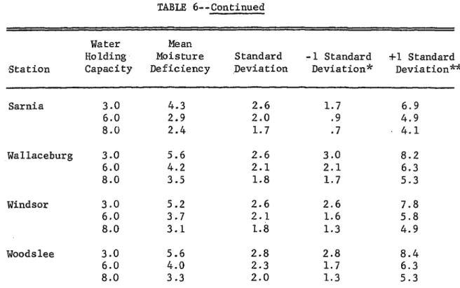
TABLE 6--Continued
Station
Water Holding Capacity
Mean Moisture Deficiency
Standard Deviation
-1 Standard Deviation*
+1 Standard Deviation*
Sarnia 3.0 4.3 2.6 1.7 6.9
6.0 2.9 2.0 .9 4.9
8.0 2.4 1.7 .7 ■ 4.1
Wallaceburg 3.0 5.6 2.6 3.0 8.2
6.0 4.2 2.1 2.1 6.3
8.0 3.5 1.8 1.7 5.3
Windsor 3.0 5.2 2.6 2.6 7.8
6.0 3.7 2.1 1.6 5.8
8.0 3.1 1.8 1.3 4.9
Woodslee 3.0 5.6 2.8 2.8 8.4
6.0 4.0 2.3 1.7 6.3
8.0 3.3 2.0 1.3 5.3
* 83.5 per cent of all cases are greater than -1 Standard Deviation.
41
soils. The degree of deficiency becomes less in the more humid areas
of the region but the danger of invisible drought is still present.
Monthly Deficiency
Crops vary as to the time when a water deficiency will be most
harmful or when they can best resist a deficiency. A deficiency of
moisture during the early stages of growth for corn will delay silking,
tasseling, and maturity. If by tasseling"^ time the water deficit is
overcome and moisture is available for the remainder of the growing £
season the crop yield will not be seriously damaged.
A moisture deficiency during silking and tasseling will greatly
decrease the yields of corn. Experiments in Washington found that a
depletion of available moisture during silking and tasseling decreased
yields by 22 to 50 per cent.^ Following this period a moisture defi
ciency will not greatly decrease crop production. A moisture defi
ciency during the entire growing season will result in stunted plants,
slow maturity and poor yield. An experiment in Nebraska, found that
with a moisture deficiency throughout the growing season a yield of
69 bushels per acre of corn resulted, whereas under conditions of
8
adequate moisture the yields increased to 153 bushels.
In the St. Clair Region there is a moisture deficiency throughout
the growing season, with the greatest deficiency occuring during the
hot summer months when corn and other crops are at a critical stage
of growth when they need sufficient moisture to mature properly.
Figures 17 to 22 show the average deficiency over the growing season
as well as the average deficiency for each of the five months. The maps
AVERAGE WATER
DEFICIENCY
GROWING
SEASON
Inches
Less than 3 . 0
3.0- 3.4
3 .5 -3 .9
4 .0 - 4 .4
4 .5 -4 .9
V.YJ 5 . 0 - 5 . 4
5.5 and greater
43
AVERAGE WATER
DEFICIENCY
(M AY)
In c h e s
□ Less than .2 0
.2 0 and greater
4 o S CA LE 8 16
Figure 18
AVERAGE WATER
DEFICIENCY
(JU N E)
Inches
Less than . 4 0
. 4 0 - . 4 9
5 0 - . 5 9
6 0 - . 6 9
7 0 - . 7 9
,80 and greater
45
AVERAGE WATER
DEFICIENCY
Inches
(J U L Y )
^ 1.30-1.39
] 1 .4 0 -1 .4 9
1 .5 0 -1 .5 9
1.60 and greater
Figure 2 0
AVERAGE
WATER
DEFICIENCY
(AUGUST)
47
AVERAGE WATER
DEFICIENCY
Inches
.9 0 and greater
Figure 2 2
were constructed by using the Theissen polygon method to determine the
area of influence for each of the 12 climatological stations. Within
these areas moisture deficiencies were found for the various soils by
use of the water balance computer programme.
Figures 17 to 22 show a general trend of increasing moisture
deficiency from north to south. In Figure 17 the 6 inch water hold
ing capacity soils have a deficiency of less than 3.0 inches in areas
influenced by the three most northerly climatological stations, whereas
in Essex County the soils with a 6 inch water holding capacity have
deficiencies ranging from 3.5 to 4.9 inches. Figures 18 to 22 show
that the highest moisture deficiencies occur on sandy soils throughout
the region in all summer months, the least deficiencies on the silt
and clay loams especially around Windsor and in northern Lambton County.
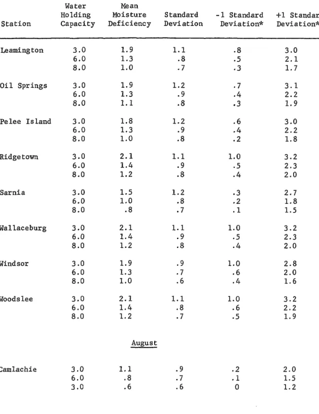
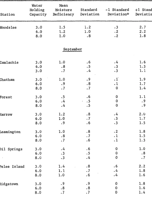
The expected frequencies and severity of water deficiency by month
for the 12 stations in the St. Clair Region are summarized in Table 7.
The most critical shortage of water occurs in the months of July and
August with a maximum average deficit at Harrow on sandy soils of 2.2
inches in July and the least for the two months at Forest with an
average deficit of 0.8 inches in both July and August. Even in the
area of least deficiency around Forest only 18 per cent of the years
recorded had no deficit in either July or August on soils of 8.0 inches
water holding capacity and only 2 per cent of the years recorded no
deficit in both months. To the other extreme Harrow recorded only 12.5
per cent of the years with no deficit in either July and August and
49
TABLE 7
VARIATIONS IN MOISTURE DEFICIENCY BY MONTH May Station Water Holding Capacity Mean Moisture Deficiency Standard Deviation -1 Standard Deviation* +1 Standard Deviation**
Camlachie 3.0 .2 .3 0 .5
6.0 .1 .2 0 .3
3.0 .1 .1 0 .2
Chatham 3.0 .3 0 .5
6.0 .1 .2 0 .3
8.0 .1 .1 0 .2
Forest 3.0 .1 .2 0 .3
6.0 .1 .1 0 .2
8.0 .1 .1 0 .2
Harrow 3.0 .3 0 .5
6.0 .1 .2 0 .3
8.0 .1 .1 0 .2
Leamington 3.0 .1 .2 0 .3
6.0 .1 .1 0 .2
8.0 .1 .1 0 .2
Oil Springs 3.0 .3 0 .5
6.0 .1 .2 0 .3
8.0 .1 .1 0 .2
Pelee Island 3.0 .1 .3 0 .4
6.0 .1 .1 0 .2
8.0 .1 .1 0 .2
Ridgetown 3.0 .3 0 .5
6.0 .1 .2 0 .3
8.0 .1 .1 0 .2
Sarnia 3.0 .3 0 .5
6.0 .1 .2 0 .3
8.0 .1 .1 0 .2
TABLE 7— Continued
May
Station
Water Holding Capacity
Mean Moisture Deficiency
Standard Deviation
-1 Standard Deviation*
+1 Standard Deviation**
Wallaceburg 3.0 .2 .3 0 .5
6.0 .1 . 1 0 .2
8.0 .1 .1 0 .2
Windsor 3.0 .3 0 .5
6.0 .1 .1 0 .2
8.0 .1 .1 0 .2
Woodslee 3.0 .3 0 .5
6.0 .1 .2 0 .3
8.0 .1
June
.1 0 .2
Camlachie 3.0 .8 .9 0 1.7
6.0 .5 . 6 0 1.1
8.0 .4 .5 0 .9
Chathan 3.0 1.0 .8 .2 1.8
6.0 .6 .5 .1 1.1
8.0 .5 .4 .1 .9
Forest 3.0 . 6 .7 0 1.3
6.0 .4 .4 0 .8
8.0 .3 .3 0 .6
Harrow 3.0 1.0 .8 .2 1.8
6.0 . 6 .5 .1 1.1
8.0 .5 .4 .1 .9
Leamington 3.0 .7 . 6 .1 1.3
6.0 .4 .4 0 .8
8.0 .3 .3 0 .6
Oil Springs 3.0 .8 .9 0 1.7
6.0 .5 .6 0 1.1