A Quick Guide to Statistical Modeling Design Defects,
Product Liability and the Protective Properties of
Suboptimal Nonparametric and Robust Statistics
Michael Lang1,∗ ID
1 Graduate School of Excellence Computational Engineering, Technische Universtät Darmstadt, Dolivostraße 15, 64293 Darmstadt, Germany; Tel.:+49 6151 1624401, Fax: 49 6151 1624404
∗Correspondence: [email protected]
Abstract: Statistical modeling lies at the heart of product design and development throughout numerous
1
engineering disciplines, especially since processing large amounts of data has become increasingly ubiquitous.
2
While mathematical statistics provide elegant guidance pertaining to the question of whether or not some
3
particular underlying modeling assumptions are justified and appropriate, when pursuing a more comprehensive
4
assessment of product design and development other considerations often increase in significance. Therefore,
5
we will examine and analyze the tedious interactions and implications of statistical modeling choices and
6
product liability exposure. To the best of our knowledge, this paper is the first to draw attention to and explore
7
some often overlooked or oversimplified dangers and pitfalls that enter the equation when product design
8
heavily relies on statistical modeling. In particular, through a diligent analysis of both statistical and legal
9
aspects we will explore how statistically optimal procedures may yield far from optimal outcomes in terms
10
of product liability when applied to actual real life problems and why suboptimal nonparametric or robust
11
approaches may constitute better alternatives.
12
Keywords: product design; design defect; robust statistics; nonparametric statistics; model uncertainty;
13
optimization; liability; tortious product liability; strict product liability
14
1. Introduction
15
IoT, Big Data, Machine and Deep Learning and related technologies first and foremost leverage the power
16
ofStatistics, a discipline which may be described as the art and science of the analysis and interpretation of
17
data. A crucial commonality encountered in all statistical endeavors lies in the necessity to impose modeling
18
assumptions, be they explicit or implicit in nature, on the observed data.
19
As will be shown in Section2and exemplified by the pitfalls of the ubiquitous Gaussian assumption, the
20
detrimental ramifications arising from an adherence to unrealistic modeling assumptions have been known for
21
centuries and eventually led to the development of the field of robust statistics and formal robustness theories in the
22
early 1960s. Somewhat ironically however, the stoic quest for optimal robust procedures made them vulnerable to
23
some of the same perils they initially set out to tackle. Nonparametric and distribution-free approaches on the other
24
hand, while being more broadly applicable, are frequently dismissed as too conservative and poor performing.
25
The main focus of this paper however is not to reiterate decades-old debates pertaining to philosophical aspects
26
of mathematical statistics, which is why Section2is exemplary and purposely non-exhaustive.
27
To the best of our knowledge, this paper is the first to draw attention to and explore some often overlooked
28
or oversimplified dangers and pitfalls that enter the equation when product design heavily relies on statistical
29
modeling. In Section3, from an engineering perspective, we will comprehensibly and exhaustively develop the
30
relevant pathways allowing for flaws in the initial modeling to yield to civil liability1for various actors involved.
31
1 wherein our focus will be on the German jurisdiction, although due to European harmonization most aspects hold for all European
Member States and can furthermore partly be extrapolated to other parts of the world.
We will emphasize that, unbeknownst to many in the engineering community, civil liability for defective products
32
cannot simply be excluded through general terms and conditions or other means and ought therefore be taken into
33
account from the very early stages of product design and development. Conceding that due to importance and
34
weight of case-specific circumstances no general solution or guidance can responsibly be provided, Section4aims
35
at providing the reader with a concise summary of the most relevant findings and some broad recommendations.
36
Finally, Section5concludes this paper with a short discussion.
37
2. Statistical Approaches
38
In the following basic concepts will be introduced together with the historical context in which they arose.
39
Customarily a distinction between parametric and nonparametric approaches is drawn, representing approaches
40
that favor efficiency over validity and vice-versa, respectively, as depicted in Table1.
41
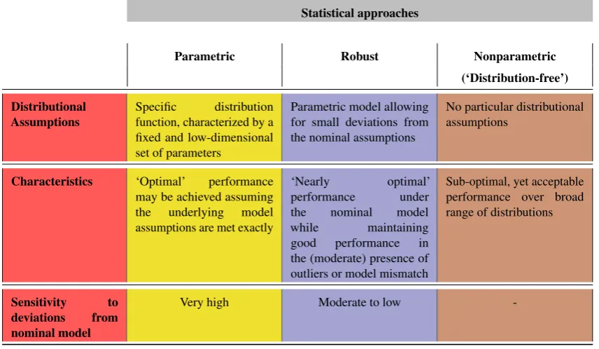
Table 1.Overview of statistical approaches: Parametric, Robust, Nonparametric
Statistical approaches
Parametric Robust Nonparametric
(‘Distribution-free’)
Distributional Assumptions
Specific distribution function, characterized by a fixed and low-dimensional set of parameters
Parametric model allowing for small deviations from the nominal assumptions
No particular distributional assumptions
Characteristics ‘Optimal’ performance may be achieved assuming the underlying model assumptions are met exactly
‘Nearly optimal’ performance under the nominal model while maintaining good performance in the (moderate) presence of outliers or model mismatch
Sub-optimal, yet acceptable performance over broad range of distributions
Sensitivity to deviations from nominal model
Very high Moderate to low
-Robust approaches, accordingly, can be thought of as pursuing a compromise between the two
42
aforementioned extremes in that they should exhibit near optimal behavior if the nominal model indeed provides
43
an accurate representation of the underlying data generating process(es) while at the same time exhibiting
44
deteriorated, yet still acceptable performance in the case of small to moderate deviations from the nominal model
45
(‘model-mismatch’) or in the case of contamination by a certain amount of (possibly arbitrarily high) extrinsic
46
disturbances (‘outliers’).
47
2.1. Normality Assumption, Maximum Likelihood and Least Squares
48
Consider the basic problem of observing a fixed but unknown valueµcontaminated by random errorsXn, 49
i.e.
50
Yn=µ+Xn (1)
withXn∼ N
0,σ2and thusYn∼ N
µ,σ2, i.e. the probability density function (p.d.f.) of the random
51
variableYis given by
52
fY(y) =
1
√
2πσexp
−(y−µ)
2
2σ2
which may also be written as fY(y;θ)withθ=
h
µ,σ2ibeing the finite set of distributional parameters
53
or distributional parameter vector that completely specifies the p.d.f. The construction of an estimator shall be
54
exemplified by illustrating the maximum-likelihood and least-squares approach to obtainµˆ.
55
2.1.1. Maximum Likelihood Estimator
56
The standard method for obtainingµˆin the above-mentioned estimation problem is given by the maximum
57
likelihood approach and was introduced by R. A. Fisher in 1922 [1]. Givenn =1,. . .,Ni.i.d. observations
58
y1,. . .,yNofYn, the joint probability density function is given by the product of the individual densities, i.e. 59
f(y1,. . .,yN;θ) = N
Y
i=1
f(yi;θ) =L(θ;y) (3)
withL(θ;y)being the likelihood function, a function of the unknown distributional parameter vectorθ
60
conditioned on the observed data sampley= [y1,. . .,yN]. The likelihood functionL(θ;y)can be interpreted as
61
pertaining to the probability of observing exactly the specific dataset at hand, i.e.y1,. . .,yN, for a particularθ. 62
Then, searching for estimatesθˆsuch thatLθˆ;yis maximized yields parameters for the assumed distribution that
63
result in the highest probability of ‘producing’ the observed data. Since the natural logarithm is a monotonically
64
increasing function, maximizing the more tractable lnL(θ;y)yields to the same result as maximizingL(θ;y).
65
Accordingly, rather than working with the likelihood function of Eq. (3) one conventionally works with the
66
log-likelihood function
67
lnL(θ;y) = N
X
i=1
lnf(yi;θ) (4)
instead. Applied to the problem formulated in Eq. (1) this yields
68
lnL(θ;y) =−N
2 ln(2π)− N
2 lnσ 2−1
2
N
X
i=1
(yi−µ)2 σ2
(5)
The so-called likelihood-equation provides the necessary condition for maximizing the log-likelihood
69
function, namely
70
∂lnL(θ;y)
∂µ =
1 σ2
N
X
i=1
(yi−µ) =0 (6)
Since
71
∂2lnL(θ;y)
∂µ2 =−
N
σ2 <0=⇒maximum (7)
holds, the maximum likelihood estimate forµis then obtained by multiplying Eq. (6) withσ2and solving
72
forµˆ, which yields
73
ˆ
µML =
1 N
N
X
i=1
yi=y (8)
2.1.2. Least Squares Estimator
74
Alternatively, one may follow a least-squares approach and construct an estimator that minimizes the`2
75
norm, i.e.
76
ˆ
µLS=arg min
µ d(µ) =arg minµ N
X
i=1
To determine the estimate that minimizes the distance function
77
d(µ) = N
X
i=1
(yi−µ)2= N
X
i=1 y2i −2µ
N
X
i=1
yi+Nµ2 (10)
one again takes the first derivative and sets it to zero
78
d0(µ) =−2
N
X
i=1
yi+2Nµ=0 (11)
and since
79
d00(µ) =2N>0=⇒minimum (12)
holds this yields
80
ˆ µLS =
1 N
N
X
i=1
yi =y (13)
Thus, if the normality assumption holds, both maximum likelihood and least squares yield the same
81
estimator, in this case the sample mean. Note that this is not generally the case.
82
2.2. History of the Normal Distribution and long-held Doubts as to the Validity of the Normality Assumption
83
The optimality of the sample mean (i.e. the arithmetic mean) as an estimate ofµin Eq. (1) should come
84
as no surprise, for the normal distribution was explicitly invoked by Gauss to justify the use of the arithmetic
85
mean. In fact, in his seminal 1809 work titled “Theoria motus corporum coelestium in sectionibus conicis solem
86
ambientium” (Latin for “Theory of the motion of the heavenly bodies moving about the sun in conic sections”), a
87
contribution to the application of mathematics to astronomy, Gauss provides that
88
It has been customary certainly to regard as an axiom the hypothesis that if any quantity has been
89
determined by several direct observations, made under the same circumstances and with equal care,
90
the arithmetical mean of the observed values affords the most probable value, if not rigorously, yet
91
very nearly at least, so that it is always most safe to adhere to it.([2] at 258)
92
Unbeknownst to some, the normal distribution was actually first introduced by Abraham de Moivre in 1733 as a
93
means of approximating the binomial distribution [3,4]. Furthermore, Irish-American mathematician Robert
94
Adrain is believed to have discovered the normal distribution independently of Gauss in 1808, concurrently
95
with his derivation of the method of least squares (the latter however bears striking resemblance to Legendre’s
96
derivation) [5].
97
In his derivation of the normal distribution Gauss built on previous attempts by Laplace to formally justify
98
the use of the sample mean as the optimal estimator for observations contaminated by random errors, an approach
99
customarily used at the time across the entire spectrum of natural sciences despite the lack of formal justification
100
[6]. While by minimizing the absolute value of the estimate’s deviation from the true value Laplace failed
101
to prove the optimality of the arithmetic mean he ended up proving the median to be the minimum-variance
102
estimator of the location parameter for the double exponential distribution2, whose p.d.f. is given by
103
fY(y) =
m
2 exp[−m|y−θ|] (14)
with 0<m<∞. Gauss was heavily influenced by Laplace’s work and about three decades later finally
104
delivered a formal justification for the use of the sample mean. As Hald (See[6] at 51) emphasizes, but for
105
2 The double exponential distribution later became known as and today commonly goes by the name of Laplacian distribution.See, e.g.
the different scaling (m/2 being replaced byh/√π), Gauss’ normal distribution is the double exponential
106
(Laplacian) distribution of Eq. (14) with the exponentm|y−θ|replaced byh2(y−θ)2withh = 1/√2σ.
107
Karlgaard remarks that “it is certainly interesting to note that minimum`1norm methods based on weighted
108
medians were in use well before the invention of minimum`2norm methods” ([7] at 6).
109
110
The ‘sacredness’ of the normality assumption is perhaps best illustrated by the following quote attributed to
111
French physicist Gabriel Lippmann by Poincaré in 1912:
112
Everyone believes in the normal distribution - Dr. Lippmann once expressed to me - the experimenters
113
because they think that it is a mathematical theorem, and the mathematicians because they think it is
114
an experimental fact.(see, e.g.[8] at 466; [9] at 20)
115
Thus, the unfoundedness of the normality assumption had clearly been known long before the advent of the
116
contemporary formal field of robust statistics (seeSection2.3). This is relevant, for it has a direct and profound
117
impact on notions such as negligence, duty of care, and perhaps most importantly, the state of scientific and
118
technical knowledge, as shall be discussed in Section??. Evidence shows that, despite its widespread use and
119
acceptance, the normality assumption has been disputed by respected scholars since the first 19th century. For
120
instance, back in 1818 Bessel in an empirical analysis of the measurement errors of astronomical observations
121
noted that they did in fact not follow Gauss’ normal distribution [7,10].
122
2.3. Contemporary Robustness Theory: Tukey, Huber and Hampel
123
The contemporary notion and use of the term ‘robustness’ was coined by George Box in his 1953Biometrika
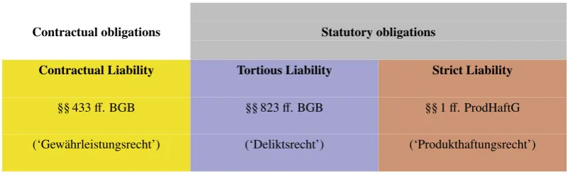
124
paper [11]. The advent of the contemporary field of robust statistics is however inextricably bound to John W.
125
Tukey, Peter J. Huber and Frank R. Hampel (in that order) [12,13].
126
2.3.1. Tukey’s 1960 Paper
127
Tukey in 1960 [14] famously drew broad attention to the fact that, when contaminating the normal
128
distribution with varying percentagesof a slightly heavier tailed distribution (in Tukey’s example a normal
129
distribution with its standard deviation increased by a factor of 3), it takes less than 1% of contamination to
130
“utterly destroy the average performance of so-called optimal estimators.” ([15] at 272)
131
132
Given some observationsxi 133
xi∼(1−)N
0,σ2+N0, 9σ2 (15)
the sample standard deviation (or root mean square deviation)
134
sn=
" 1 n
X
(xi−x)2
#1/2
(16)
and the mean deviation (or mean absolute deviation)
135
dn=
1 n
X
|xi−x| (17)
can be used as scale estimators. It turns out, however, that as soon as one contaminates the distribution of
136
xiin Eq. (15) with a fraction as tiny as =0.0018 from the heavier tailed distribution, the root mean square 137
deviation ceases to be more efficient than the mean absolute deviation and at = 0.05 the latter is twice as
138
efficient as the former (see[16] at 6). This holds for all 0.002≤≤0.5 (see[17,18] at 3;see also[16]) and
139
stands to exemplify that classical procedures are highly susceptible to even tiny deviations from the assumed
140
model. In other words, they are not distributionally robust.
2.3.2. Huber’s 1964 Minimax Approach
142
Huber’s 1964 groundbreaking paper [19] on the ‘Robust Estimation of a Location Parameter’ is commonly
143
agreed upon as the first formal and solid contribution to the modern theory of robust statistics. In said paper,
144
Huber depicts the task of constructing a robust location estimator as a zero-sum game between nature and
145
the statistician, wherein nature chooses a distribution in the neighborhood of the assumed model followed by
146
the statistician’s choice of an appropriate estimator which minimizes the asymptotic variance for the worst
147
possible case the considered neighborhood of the model allows. The neighborhood is described by the gross
148
error or-contamination model for contaminated normal distributions where a fraction of the data stems
149
from a contaminating distribution, as already encountered in Eq. (15) where the contaminating distribution is
150
N0, 9σ2. Huber solves the posed minimax problem by introducing a new class of asymptotically normal and
151
consistent generalized maximum likelihood estimators, called M-estimators.
152
153
As previously discussed in Section 2.1.1, the maximum likelihood estimate is obtained by solving for
154
the value that maximizes the log-likelihood function of the data, i.e. given observationsx1,. . .,xNfrom the 155
corresponding density fX(x;µ)one obtainsµˆMLas
156
ˆ
µML=arg max
µ N
X
i=1
lnfX(xi;µ) (18)
or equivalently by solving
157
N
X
i=1
∂lnfX(xi;µ)
∂µ =0 (19)
Huber generalizes this by instead solving
158
ˆ
µM=arg min
µ N
X
i=1
ρ(xi−µ) (20)
or equivalently by solving
159
N
X
i=1
ψ(xi−µˆM) =0 (21)
withψ=ρ0being the score-function. Note that while choosingρ=−lnf
X(x)andψ=−fX(x) 0/fX(x) 160
yields the maximum likelihood estimator as a particular case of the M-estimator, the latter is more general in
161
that the score functionψis not required to be the derivative of someρ-function with respect to the parameter of
162
interest. An importantρ-function is the so-called Huberρ-function
163
ρ(x) =
1 2x
2 |x| ≤c
Hub
cHub|x| −
1
2c2Hub |x|>cHub
(22)
with the correspondingψ-function
164
ψ(x) =
x |x| ≤cHub
cHubsign(x) |x|>cHub
(23)
Note that the limit cases ofcHub→ ∞andcHub→0 correspond to the sample mean and the sample median,
165
respectively. Accordingly,µˆMrepresents an intermediate between mean and median [19–21]. In simple cases,
166
such as the one-dimensional location estimation considered here, the aforementioned game between nature and
167
the statistician has an explicit asymptotic minimax solution. In fact, the M-estimator of Eq. (22) is the maximum
168
likelihood estimator corresponding to a unique least favorable distribution with density
169
f0(x) = (1−) (2π) −1
which behaves like a normal distribution for smallxand like an exponential distribution for larger values of
170
x(see, e.g.[13,17,19]).
171
172
Comparing ML and M estimators, the crucial difference is thatρML=−lnfX(x)andψML=−fX(x) 0/fX(x) 173
are unbounded whileρM is quadratic in the middle and linear in the tails resulting in a score functionψM
174
bounded bycHubwhere 1.0≤cHub≤2.0 will give acceptable results for all≤0.2 (see[19] at 82). A commonly
175
used value iscHub=1.345. It is in fact the boundedness ofψwhich makes the M-estimator robust [13,17,19–21].
176
2.3.3. Hampel’s Infinitesimal Approach
177
An intuitive approach to assess the influence of an arbitrary data pointxon a statistic computed on a sample
178
was proposed by Tukey [22] in form of the sensitivity curve (SC). Given a sample x1,. . .,xn−1drawn from
179
N0,σ2by adding an additional arbitrary data pointxthe sensitivity curve for the sample meanxn= 1nPni=1xi 180
is
181
S Cn(x) =
(x1+x2+· · ·+x)/n−xn−1
1/n =x−xn−1 (25)
a linear function inx(see[20] at 17). The limit ofS Cn(x)forn → ∞then represents the asymptotic 182
influence of the additional arbitrary data point x on the sample mean. S Cn(x) however is generally 183
sample-dependent (see[20] at 17). Hampel in his 1968 Ph.D. thesis [23] and 1974 paper [24] introduced a more
184
versatile notion in form of the influence function (IF), broadening the SC to more general types of estimators
185
through the use of functionals.
186
187
Let Fn denote the empirical distribution function of the sample x1,. . .,xn and θˆ = (x1+· · ·+xn)/n 188
the sample mean. Expressed as functional this would beθˆ(Fn) =R xdFn(x). Hampel’s IF is defined as 189
IFx,θˆ,F= lim
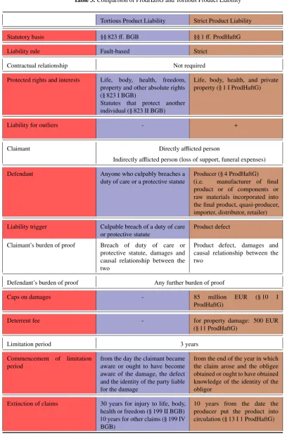
→0
ˆ
θ((1−)F+∆x)−θˆ(F)
(26)
where∆xdenotes point-mass 1 atx. That is, the IF expresses the difference of the estimator following the
190
contaminated distribution and the estimator following the nominal (uncontaminated) distribution standardized
191
by the fraction of contamination as said fraction of contamination goes to zero. For M-estimators the influence
192
function is proportional to the definingψ-function. Hampel showed that
193
bias,θˆ,F'sup
x
|IFx,θˆ,F| (27)
i.e. the asymptotic bias of an estimator with bounded influence function is bounded as well (see, e.g.[9] at
194
176; [20] at 18).
195
2.3.4. The Breakdown Point
196
An important ‘limitation’ of Hampel’s influence function is that it only describes the local stability
197
of an estimator (or, more technically, “the infinitesimal stability of (the asymptotic value of) an estimator”
198
[9] at 96). Accordingly, as Hampel points out in the same paragraph, “it must be complemented by a
199
measure of the global reliability of the estimator, which describes up to what distance from the model
200
distribution the estimator still gives some relevant information.” The Breakdown Point (BP) is one - and by
201
any means the most popular and best comprehensible - such measure. Loosely speaking, the breakdown
202
point provides the minimum amount of contamination necessary for the estimator to produce arbitrarily
203
large changes to the estimate. Put differently, it is the maximum amount of contamination an estimator
204
can withstand before it breaks down, i.e. before its bias becomes arbitrarily large. Apparently then the
205
breakdown point can take any value between 0 and 0.5, for beyond 50% contamination it is no longer
206
possible to differentiate between the nominal and the contaminating distribution(s). It shall be noted though
207
that despite its apparent tangibility, the BP is subject to some controversy in the statistical literature (see, e.g.[25]).
209
The asymptotic breakdown point (ABP) ∗ of a sequence of estimators Tn for parameter θ ∈ Θ at 210
probabilityFis defined by
211
∗
:=sup{≤1; there is a compact setK $Θ s.t. π(F,G)< =⇒G({Tn∈K}) n→∞
−→ 1} (28)
withπbeing the Prohorov distance (see[9] at 97).
212
213
The finite sample breakdown point (FSBP)n∗of the estimatorTnat sample(x1,. . .,xn)is given by
214
∗
n(Tn;x1,. . .,xn):=
1
nmax{m; maxi1,...,im
sup
y1,...,ym
|Tn(z1,. . .,zn)|<∞} (29)
where the sample(z1,. . .,zn)is obtained by replacing themdata pointsxi1,. . .,xim by the arbitrary values 215
y1,. . .,ym(see[9] at 98). In many cases, taking limn→∞n∗yields the ABP∗.
216
217
It is worth noting that the FSBP of Eq. (29) differs from the one proposed by Donoho and Huber [26]
218
in that, e.g., the latter yields 1/nfor the sample mean whereas the FSBP of Eq. (29) yields 0. This is due to
219
Donoho and Huber taking the smallestmfor which the maximum supremum of|Tn(z1,. . .,zn)|is infinite, 220
resulting in their FSBP yielding∗n+1/n(again,see[9] at 98).
221
2.4. Nonparametric Statistics
222
The limited ability to adequately represent real-world circumstances is a drawback inherent to all
223
low-dimensional parametric models, a fact which is nicely illustrated by Härdle’s analogy to the Greek
224
mythological figure ofProcrustes3. Somewhat paraphrasing Härdle, one may think of the conventional parametric
225
modeling approach as akin to projecting the observed data onto a Procrustean bed of fixed parametrization,
226
recklessly disregarding that “the preselected parametric model might be too restricted or too low-dimensional to
227
fit unexpected features” ([27] at 5). Accordingly, switching the normal distribution for another low-dimensional
228
parametric probability distribution would in essence be akin to Procrustes switching to his alternative torture
229
bed, shifting and perhaps slightly ameliorating the problem, yet remaining far from reaching a more universally
230
acceptable solution.
231
2.4.1. Clearing up Some Definitions
232
Labels such as ‘robust’, ‘nonparametric’ and ‘distribution/model free’ are not as clearly defined as one
233
might expect, which has led to rather frequent ambiguities and misclassifications (see, e.g. [18] at 6-7). The
234
following classification therefore appears in order:
235
• Robust Proceduresare essentially parametric procedures that have been “hardened” so as to allow for (small)
236
deviations from the assumed nominal model. At their core, however, they remain parametric methods, i.e.
237
they are based on the explicit or implicit assumption of a clearly defined model which is fully described by
238
a rather low-dimensional set of parameters (e.g.[µ,σ]for the normal distribution).
239
• Nonparametric Procedureson the other hand are different in that no such restrictive assumptions are made.
240
In fact, one may interpret nonparametric statistics as being ‘infinitely dimensional parametric’. However,
241
certain assumptions are commonly encountered in nonparametric statistics as well, e.g. that the data sample
242
3 Procrustes (‘the stretcher’), was a Greek robber who would lure unsuspecting travelers into his house by promising them a nice meal
is a sequence of independent and identically distributed (i.i.d.) random variables and/or that the set of
243
possible probability densities be restricted to symmetric ones.
244
• Distribution-free Proceduresare test statistics whose null distribution does not depend on the probability
245
distribution from which the sample was drawn, i.e. the sampling distribution under the null is the same
246
for all possible underlying distributions. Estimates derived from such tests are also commonly referred to
247
asdistribution-free, even though this is generally not true (see, e.g.[18] at 6-7). Nevertheless, the terms
248
‘nonparametric’ and ‘distribution-free’ are often used interchangeably (see, e.g.[28] at 114).
249
2.4.2. Some Basic Nonparametric Procedures
250
Nonparametric procedures often rely on rank transformation of the data, i.e. the observed data points are
251
replaced by their respective ranks. Even more basic is the sign-test proposed by Arbuthnot [29] back in 1710 to
252
refute the claim that newborns were equally likely to be male and female [30,31]. Givennobservations from a
253
population which may be discrete or continuous and need not be symmetric, one hypothesizes that the median
254
under the null be, sayM0and then counts the number of observations exceedingM0. The null and the alternative
255
both follow a binomial distribution and ifH0 : M= M0holds, the number of values smaller thanM0will have
256
a binomial distribution with parametersnandp=0.5 and the counted number of observations greater thanM0
257
may then be used as an alternative equivalent statistic in a one or two-tail test (see, e.g.[30], p. 1316). While the
258
basic sign-test is neither particularly efficient nor powerful, it shall be emphasized that it does not assume a
259
symmetric population.
260
261
Arguably however, the advent of the modern era of nonparametric tests can be traced back to seminal
262
contributions by Wilcoxon [32] in 1945, Mann and Whitney [33] in 1947, and Hodges and Lehmann
263
[34] in 1956. Specifically, Wilcoxon proposed the Wilcoxon signed rank test for medians of symmetric
264
distributions and the Wilcoxon rank sum test for the difference in medians and Mann and Whitney showed
265
the rank sum test to be equivalent to the sign-test for pairwise differences across the two samples while
266
Tukey in 1949 showed that the Wilcoxon signed rank test is equivalent to the sign test when applied to
267
pairwise averages from the samples, which Tukey referred to as Walsh-averages (see, e.g.[31] at 2). Hodges
268
and Lehmann [34] showed that the asymptotic relative efficiency (ARE) of the Wilcoxon tests compared
269
to t-tests is>0.864. Specifically, the ARE is 3/π=0.955 at the normal and has in general no upper limit [30,31].
270
271
For the sake of brevity and for better comparison to robust procedures discussed earlier, the discussion
272
of nonparametric procedures in this Section shall be limited to R-estimators. For a in depth appraisal the reader
273
is referred to, e.g. [28,35–37].
274
2.4.3. R-Estimators
275
Roughly speaking, procedures based on rank statistics require less restrictive assumptions regarding the
276
underlying distribution and are inherently robust against distributional departures such as misspecified models,
277
contamination and outliers. Furthermore, these inherent robust properties are generally globally robust as opposed
278
to conventional robust statistics (e.g. M-estimators) which are rather locally robust (see, e.g.[37] at 91).
279
In their seminal 1963 paper [38] Hodges and Lehmann built on the prior art by Wilcoxon, Tukey, Mann,
280
and Whitney outlined in Section2.4.2and proposed a class of robust estimators based on rank tests commonly
281
referred to as R-estimators. Most importantly, they were able to show that these estimators inherit the desirable
282
robustness and efficiency aspects of the rank tests they are based on. While originally being derived from
283
one-sample tests (cf.[38]), it has become more customary to introduce them following an approach based on
284
two-sample test (see, e.g.[9,17]). Below the derivation found in [17] will be followed.
285
286
Consider two independent samples(x1,. . .,xm) ∼ F(x)and(y1,. . .,yn) ∼G(x)withG(x) = F(x−∆), 287
i.e. withG(x)equal to F(x)but for an unknown location shift ∆. Let the two samples be merged into a
288
1≤i≤m+nbe some given scores (weights). One may then test for∆ =0 against∆>0 based on the test
290
statistic
291
Sm,n=
1 m
m
X
i=1
a(Ri) (30)
with scoresaigenerated by some functionJ 292
ai= (m+n)
Z i/(m+n)
(i−1)/(m+n)
J(s)ds (31)
with
293
Z
J(s)ds=0 (32)
and accordingly
294
X
ai=0. (33)
Under the null hypothesis of∆=0 the expected value of Eq. (30) is then 0.
295
296
In the following, let m = n for the sake of simplicity. Eq. (30) expressed in terms of functionals
297
reads as
298
S (F,G) =
Z J
" 1 2F(x) +
1 2G(x)
#
F(dx) (34)
and by substitutingF(x) =s
299
S(F,G) =
Z J
" 1 2s+
1 2G
F−1(s)
#
ds (35)
Note how Eq. (35) together with Eq. (31) yields Eq. (30).
300
301
An R-estimator of location Tn and shift∆n can be derived by adjusting ∆n such that Eq. (30) computed 302
for samples (x1,. . .,xn) and (y1−∆n,. . .,yn−∆n) becomes as close to zero as possible, i.e. Sn,n ≈ 0. 303
In the one-sample case one adjusts TN such that Sn,n ≈ 0 when computed for samples (x1,. . .,xn) and 304
(2Tn−x1,. . ., 2Tn−xn), i.e. the missing second sample is replaced by a mirror image of the first sample 305
wherein eachxiis replaced byTn−(xi−Tn) = 2Tn−xi. Put differently,Sn,n ≈0 means that one adjusts or 306
rather shifts the second sample, either through∆nin the two-sample case orTnin the one-sample case, such that 307
a difference between the two is no longer discernible.
308
309
The location estimatorTnthus derives from a functionalT(F), defined by the implicit equation 310
Z J{1
2 h
s+1−F2T(F)−F−1(s)i}ds=0 (36) (see, e.g.[17] at 62; [9] at 111).
311
312
The Wilcoxon test, J(t) = t− 1
2 e.g. yields the Hodges-Lehmann estimates ∆n = med{yi−xj} and
313
Tn=med{12(xi+xj)}. 314
315
The score generating functionJ(t)shall be assumed to be symmetric, i.e.
316
and a functionU(x)shall be introduced as the indefinite integral of
317
U0(x) =J0{1
2[F(x) +1−F(2T(F)−x)]}f(2T(F)−x). (38) The influence function of the R-estimator can then be shown to be
318
IF(x;F,T) = U(x)−
R
U(x)f(x)dx R
U0(x)f(x)dx (39)
which for symmetricF, which in turn impliesU(x) =J(F(x)), simplifies to
319
IF(x;F,T) =R J(F(x))
J0(F(x)) f(x)2dx (40)
(see[17], Section 3.4).
320
321
For a monotone and integrable J for which T(F) is uniquely defined, T is continuous at F and the
322
breakdown point∗is given the value offor which
323
Z 1−/2
1/2
J(s)ds=
Z 1
1−/2
J(s)ds (41)
(see, e.g.[17] at 67; [9] at 112).
324
325
Accordingly, the Hodges-Lehmann estimator of location J(t) = t− 12, i.e. the median of pairwise
326
averages, has a breakdown point of
327
∗
=1− √1
2
≈0.293 (42)
which is to be considered reasonably high.
328
3. Civil Liability for Product Defects
329
In the following the distinct mechanisms and ramifications arising from the three main liability constructs,
330
which are depicted in Table2, will be analyzed and necessary and up-to-date references to case law to interpret
331
and apply them correctly will be provided. In doing so, a self-contained and concise, yet exhaustive picture
332
of these extensive areas of civil law is developed, thereby removing the requirement of prior knowledge of
333
the subject matter on the part of the reader. In essence, all statutory provisions of relevance to the discussions
Table 2.Overview of the three main liability constructs for defective products
Liability for defective products
Contractual obligations Statutory obligations
Contractual Liability Tortious Liability Strict Liability
§§ 433ff. BGB §§ 823ff. BGB §§ 1ff. ProdHaftG
(‘Gewährleistungsrecht’) (‘Deliktsrecht’) (‘Produkthaftungsrecht’)
334
in this work are those of the special part of the law of obligations (‘Schuldrecht - Besonderer Teil’) and the
335
Product Liability Act (‘Produkthaftungsgesetz’). There is however a caveat to that. For these sections are not
self-contained but have to be interpreted in the broader context of the code due to provisions included by reference.
337
It will be shown that these distinct liability constructs are not mutually exclusive, but coexist and can be applied
338
in parallel. An awareness and understanding of these liability mechanisms is therefore of paramount importance
339
and ought to be incorporated into and influence all stages of research, product design and development.
340
3.1. Contractual Liability
341
Civil liability for product defects is part of the law of obligations where in turn a fundamental distinction
342
between contractual obligations (‘vertragliche Haftung’) and statutory obligations (‘gesetzliche Haftung’) shall
343
be made. The former, as the term implies, requires a contractual relationship between the parties while the latter
344
covers faulty conduct (‘Verschuldenshaftung’) as well as strict (as for there is no fault requirement) liability
345
(‘Gefährdungshaftung’)
346
Thus, before discussing the arguably more important matters of tortious product liability (‘deliktische
347
Produzentenhaftung’) and strict product liability (‘Produkthaftung nach ProdHaftG’) attention shall briefly be
348
directed to contractual liability.
349
3.1.1. Requirements
350
For a contractual liability to attach the prerequisite of the existence of a valid sales contract between buyer
351
and seller has to be satisfied. Depending on whether the relationship is “Business to Consumer” (B2C) or
352
“Business to Business” (B2B) laws pertaining to purchase agreements (‘Kaufvertragsrecht’) or to contracts to
353
produce a work (‘Werkvertragsrecht’) apply, for the B2C and B2B scenarios, respectively. Typical contractual
354
duties in a purchase agreement are listed in § 433 BGB and in § 631 BGB for a contract to produce a work.
355
3.1.2. Material and Legal Defects
356
§ 433 I 2 BGB states that the seller must procure the thing for the buyer free from material and legal defects.
357
It shall be emphasized that in this context the term defect is subject to a wide interpretation. As one would
358
expect, § 434 I 1 BGB states that in order to be considered free of material defects the thing, upon the passing
359
of risk (‘Gefahrenübergang’), has to be of the agreed quality. The legislator’s broad interpretation of the term
360
defect however becomes apparent in § 434 I 2 BGB which specifies that, in case the quality has not clearly been
361
articulated in the respective contractual agreement, the thing has to be suitable for the use intended under the
362
contract (§ 434 I 2 No. 1 BGB) or it has to be suitable for the customary use and of the quality a reasonable buyer
363
would expect from a product of this kind (§ 434 I 2 No. 2 BGB). The legislator goes on to further clarify that
364
quality under § 434 I 2 No. 2 BGB includes expectations reasonably induced in the buyer by advertisement or
365
public statements concerning product characteristics made by the seller, the producer or vicarious agents of either
366
one (§ 434 I 3 BGB).
367
The product, on the other hand, is considered free of ‘legal defect’ if pertaining to the purchase third
368
parties can either assert no rights at all or only assert such rights appropriated by the buyer in the underlying
369
contractual agreement (§ 435 BGB) Klindt et al. [39] provide the example of a software that was sold even
370
though it incorporates and uses proprietary libraries without the appropriate license. This would constitute a
371
textbook example of a ‘legal defect’ of the product as the rights holder may bring actions against the buyer of
372
said software product.
373
For B2B scenarios the notion of material and legal defect is defined analogously in § 633 BGB. For the sake
374
of brevity the following discussion will mainly consider B2C scenarios.
375
3.1.3. The Special Case of Software
376
Even though the legal community widely accepts the fact that due to the intrinsically complex nature of
377
software products an absolute absence of material defects cannot be achieved according to the prevailing opinion
378
this shall not justify a deviation from the generally accepted and above stated definitions of what constitutes a
product defect4. In a 2006 landmark decision5the BGH, among other things, found software to be a thing in
380
terms of § 90 BGB for which depending on whether the goods were surrendered subject to a purchase or a lease
381
agreement sales or tenancy laws are to be applied, respectively. Note that § 90 BGB states that only corporeal
382
objects are things as defined by law, a definition that at first sight would exclude software products. However
383
the court argued that for the software to be of any actual use it necessarily had to be materialized on some sort
384
of storage medium thereby satisfying the corporeal object requirement. This is consistent with previous BGH
385
decisions regarding the composition of software6.
386
3.1.4. Legal consequences of defects
387
The rights granted by the legislator to the buyer of a defective product are manifold (see, e.g.[40] for an
388
exhaustive discussion of the matter).
389
390
§ 437 BGB states that the buyer may:
391
1. demand cure under § 439 BGB
392
2. revoke the purchase under §§ 440, 323, 326 V BGB
393
3. reduce the purchase price under § 441 BGB
394
4. demand damages under §§ 440, 280-283, 311a BGB
395
5. demand reimbursement of futile expenses under § 284 BGB
396
3.1.5. Boundaries on the Exclusion of Contractual Liability
397
In light of the above considerations it may appear tempting to exclude or limit liability by resorting to
398
contractual provisions. However, the legislator imposed strict boundaries on such practices. Generally speaking,
399
as far as contracts go, the crucial distinction to keep in mind is between individually negotiated terms of contract
400
(‘Individualvertrag’) on one hand and general terms and conditions (‘Allgemeine Geschäftsbedingungen’ - AGB)
401
on the other hand. While the legislator imposes relatively few and very basic boundaries on the former (e.g.
402
violation of morality (‘Sittenwidrigkeit’) as in § 138 BGB), the latter are heavily regulated (§§ 305ff. BGB).
403
§ 305 I 1-2 BGB define general terms and conditions as
404
all contract terms pre-formulated for more than two contracts which one party to the contract (the
405
user) presents to the other party upon the entering into of the contract. It is irrelevant whether
406
the provisions take the form of a physically separate part of a contract or are made part of the
407
contractual document itself, what their volume is, what typeface or font is used for them and what
408
form the contract takes.
409
Clearly, in practice the vast majority of contracts will fall into this category. On the other hand, contract terms do
410
not become standard business terms to the extent that they have been negotiated in detail between the parties
411
(§ 305 I 3 BGB) and individually agreed terms take priority over standard business terms (§ 305b BGB). Caution
412
is required though due to the BGH’s very strict interpretation of what does and does not constitute a valid
413
negotiation for the sake of eventually obtaining a valid individual contractual agreement. In fact, according to
414
consistent decisions by the BGH merely ‘negotiating’ contractual provisions does not suffice, rather an act of
415
bargaining is required7.
416
417
For general terms and conditions to be validly incorporated the contracting party needs to acknowledge and agree
418
to them (§ 305 II BGB). Surprising and ambiguous clauses are void by law (§ 305c I BGB) and if doubts in the
419
interpretation arise they are resolved against the user of the pre-formulated terms and conditions (§ 305c II BGB).
420
The rules in §§ 305ff. BGB apply regardless of possible attempts to circumvent them by other constructions
421
(§ 306a BGB). The legislator severely limits the user’s ability to exclude liability. According to § 307 I BGB
422
provisions are ineffective if, contrary to the requirement of good faith, they unreasonably disadvantage the other
423
party to the contract with the user. An unreasonable disadvantage may also arise from the provision not being
424
clear and comprehensible. Furthermore, § 309 BGB explicitly forbids the exclusion of liability for injury to
425
life, body or health and in case of gross fault (§ 309 No. 7 BGB) as well as other exclusions of liability for
426
breaches of duty (§ 309 No. 8 BGB) - of particular relevance here those pertaining to defects in contracts relating
427
to the supply of newly produced things and relating to the performance of work where provisions excluding
428
liability for defects overall or in regard to individual parts are void by law as are those limiting to the granting
429
of claims against third parties or made dependent upon prior court actions (§ 309 No. 8 aa) BGB). It is also
430
worth mentioning that the recent addition of § 309 No. 14 to the German Civil Code specifies that provisions
431
mandating an attempt of Alternative Dispute Resolution (ADR) to have been undertaken and failed prior to the
432
filing of a claim against the user are also explicitly forbidden8.
433
3.2. Tortious Product Liability
434
We can think of the special part of the law of obligations (‘Schuldrecht Besonderer Teil’) as having two
435
main pillars:
436
(i) ‘contractual obligations’ (‘vertragliche Schuldverhältnisse’)
437
(ii) ‘statutory obligations’ (‘gesetzliche Schuldverhältnisse’)
438
of particular relevance to the matter at hand, the ‘law of unlawful actions’ (‘Recht der unerlaubten
439
Handlungen’ or ‘Deliktsrecht’)
440
While implications of the former were discussed in the previous section, in this section the focus will be on the
441
latter, also known as ‘the law of torts’. Broadly speaking, a tort is a civil wrong other than a breach of contract
442
for which damages can be recovered.
443
3.2.1. The German Law of Torts, §§ 823-853 BGB
444
There are three ‘general provisions’ in the German law of torts, namely §§ 823 I, 823 II and 826 BGB, of
445
which § 823 I is generally regarded as being the most significant. The sections read as follows:
446
§ 823
447
(1) A person who, intentionally or negligently, unlawfully injures the life, body, health, freedom,
448
property or another right of another person is liable to make compensation to the other party for the
449
damage arising from this.
450
(2) The same duty is held by a person who commits a breach of a statute that is intended to protect
451
another person. If, according to the contents of the statute, it may also be breached without fault,
452
then liability to compensation only exists in the case of fault.
453
454
§ 826
455
A person who, in a manner contrary to public policy, intentionally inflicts damage on another person
456
is liable to the other person to make compensation for the damage.
457
Contrary to specific product liability acts, the delict provisions of the BGB, i.e. §§ 823-853, are not specifically
458
intended to address product liability matters but are general tools for the claimant to seek compensation for
459
damages that arose from the infringement of one or multiple of the claimant’s absolute rights by a tortfeasor’s
460
faulty conduct. ‘Absolute rights’ are ‘erga omnes’ (Latin for ‘towards all’) rights, i.e. “rights which can be
461
interfered with by everyone and which can be asserted against everyone” ([41], p. 69). In contrast, ‘relative
462
8 § 309 No. 14 BGB as introduced by the amendment of the German Civil Code, effective February 26th, 2016, cf. BGBl I Nr. 9/2016, S.
rights’ would be rights that can only be asserted on the basis of an existing legal relationship, e.g. rights that can
463
be asserted by one party against other parties it has entered into a binding contractual agreement with.
464
§ 823 I and § 823 II are by far the most relevant delict provisions pertaining to product liability matters. Of
465
minor importance is § 826, which is distinct in that it allows for the recovery of purely economic loss, provided
466
that the damage was inflicted intentionally (i.e. willfully and ‘not just negligently’) and “in a mannercontra
467
bonos mores” ([41] at 15). The recovery of purely economic loss is not possible under § 823 I but it is under
468
§ 823 II. The actual applicability of § 826 compared to §§ 823 I,II is severely limited by factual prerequisites of
469
an intentional infliction that furthermore has to becontra bonos mores.
470
3.2.2. Fault-based Product Liability under Tort Law
471
§ 823 I BGB provides that damages arising from the intentional or negligent, unlawful injury to life,
472
body, health, freedom, property or other absolute rights of another person are to be compensated by the wrongdoer.
473
474
We point out that
475
1. The statute is applicable only to infringements committed by a person (physical or legal) to the detriment of
476
another person’s rights or interests, provided they are one of the rights or interests explicitly listed by the
477
statute or included by reference to the person’s ‘other (absolute) rights’, as discussed earlier.
478
2. No contractual or semi-contractual relationship between the parties is required.
479
3. Damages must arise from the wrongdoers faulty conduct (‘Verschuldenshaftung’), i.e. the conduct has to be
480
willful/intentional (‘vorsätzlich’)9or negligent (‘fahrlässig’)10.
481
4. The conduct must furthermore be unlawful. According to the prevailing opinion this requirement is
482
regularly met whenever a person’s absolute rights are infringed absent a legally recognized justification
483
(‘Rechtfertigungsgrund’).
484
5. There must be an adequate causal link between the claimant’s damages and the defendant’s conduct, either
485
through an active act (‘Aktives Tun’) or through an act of omission (‘Unterlassen’).
486
Liability arising from acts of omissions evidently deserve careful consideration in the area of products liability.
487
For it may be argued that in the ordinary course of events, an infringement of protected rights or interests by the
488
manufacturer due to negligent or intentional omission is more likely than due to active wrongdoing. This leads us
489
to the central notion of duty of care (Verkehrssicherungspflicht) pertaining to § 823 I.
490
3.2.3. Duty of Care (§ 823 I BGB)
491
The following duties of care have been established by German case law
492
1. Liability for defective design (‘Konstruktionsfehler’)
493
494
The manufacturer has to design the product such that to his best abilities and under reasonable
495
economic feasibility constraints, no unreasonably unsafe or dangerous product with respect to the current
496
scientific and technological knowledge will be placed on the market. The manufacturer is also expected to
497
anticipate and take into account the (potentially improper) use of its product outside the intended scope and
498
by users other than those it was originally intended for and marketed to if he knew or ought to have known
499
that such scenarios were conceivable.
500
501
2. Liability for defects in manufacture (‘Fabrikationsfehler’)
502
503
9 The definition of intention and negligence is provided by § 276 BGB which states that the obligor is responsible for intention and
negligence, if a higher or lower degree of liability is neither laid down nor to be inferred from the other subject matter of the obligation, including but not limited to the giving of a guarantee or the assumption of a procurement risk. The provisions of § 827 and § 828 apply with the necessary modifications. (§ 276 I BGB)
Presuming the absence of design defects, defective products may still result from irregularities in
504
the manufacturing process itself, e.g. due to human error or defective machinery. To address this, adequate
505
quality control measures and policies must be implemented and enforced to ensure the adherence to
506
established quality and safety standards. It is evident though that defects of individual products can never
507
be completely avoided, despite all quality control mechanisms and safeguards.
508
In this context it is important to emphasize that the manufacturer is not liable for ‘outliers’ (‘Ausreißer’), i.e.
509
single defective products, provided he undertook reasonable and adequate efforts to avoid them or at least
510
to detect them and hinder the afflicted products from leaving the manufacturer’s ‘sphere of control’. As
511
shall be explained in Section3.3, the ‘outlier-defense’ can however only be invoked to exculpate oneself
512
from tortious liability whereas the manufacturer will still be held strictly liable under ProdHaftG.
513
514
3. Liability for defective instruction (‘Instruktionsfehler’)
515
516
The manufacturer is obliged to clearly warn from dangers arising from the use of its product,
517
especially if used as intended and if the danger is not immediately discernible. Depending on the level of
518
danger and the foreseeability of misuse or improper use giving rise to said danger, the duty to make users
519
aware may also expand to encompass use cases outside the product’s intended use.
520
Warnings have to be articulated clearly and unambiguously and, depending on the severity of the danger, be
521
further emphasized and highlighted. There is however no duty to warn from obvious dangers of which the
522
user knew or ought to have known. The manufacturer may also be obliged to amend the original warnings
523
and/or instructions provided with the product if new facts come to light that would call for such an action.
524
525
4. Liability arising from a breach of organizational duty (‘Verletzung der Organisationspflicht’)
526
527
The manufacturer is generally obliged to implement organizational measures and procedures so
528
as to avoid the establishment of sources of potential dangers to the best of his ability. This duty overlaps
529
with other duties of care imposed onto the manufacturer, be they statutory or established by case law.
530
531
5. Liability for development risk (‘Verletzung der Produktbeobachtungspflicht’)
532
533
The manufacturer shall monitor for and react to new evidence pertaining to possible dangers
534
arising from use of the product. Case law established that, under certain conditions, this duty also
535
encompasses products by other parties (e.g. accessories) that, when used in combination with the product
536
may give rise to dangers. Depending on the severity of the newly discovered danger the manufacturer may
537
even be obliged to proceed with a product recall.
538
3.2.4. Burden of Proof
539
In German tort law - in particular pertaining to §§ 823 I,II BGB - an alleviation of the burden of proof has
540
been established by case law. For the courts acknowledged it would regularly amount to an undue burden (or
541
even be infeasible) for the claimant to prove the alleged tortfeasor’s fault (i.e. to establish that the conduct that
542
led to the damages was intentional or negligent), as would be required following a strict interpretation of the law.
543
It has therefore been established that providing so-calledprima facie(Latin for ‘at first sight’) evidence for the
544
alleged tortfeasor’s fault and the causal relationship to the damages claimed suffices as long as no compelling
545
contradictory explanation or evidence surfaces [42]. Pertaining to tortious product liability in particular, said
546
alleviations eventually culminated into a full shift of the burden of proof (‘Beweislastumkehr’) in favor of the
547
claimant. According to both case law upheld and established by the BGH and prevailing scholarly opinion said
548
reversal in product liability matters is just, for the burden on the claimant would otherwise be disproportionate,
549
especially in face of today’s complex and intricate (distributed) manufacturing processes [41–44].
550
It may therefore be argued that tortious product liability, which as a matter of principle is based on
552
faulty conduct, has effectively been tilted towards strict liability [41–43].
553
3.2.5. Statute of Limitations and Caps on Damages
554
The general limitation period of the BGB, i.e. three years under § 195 BGB, applies and according to § 199
555
I BGB begins with the end of the year in which the claim arose (§ 199 I No. 1 BGB) and the obligee obtains
556
knowledge of the circumstances giving rise to the claim and of the identity of the obligor, or would have obtained
557
such knowledge if he had not shown gross negligence (§ 199 I No. 2 BGB). It may be interrupted according
558
to § 204 BGB on the suspension of limitation periods as a result of the prosecution of rights. There are some
559
exceptions however imposing longer but absolute (as in they begin on the date on which the act, breach of
560
duty or other event that caused the damage occurred irrespective of the particular manner in which they arose
561
and the knowledge thereof) limitation periods of either thirty years for injury to life, body, health or freedom
562
(§ 199 II BGB) or ten years for most other claims (§ 199 IV BGB). The reason for claims eventually becoming
563
statute-barred is to provide legal certainty for all parties involved.
564
There are no caps on damages in the German law of torts. This constitutes a major differentiating factor
565
with respect to other constructs, e.g. specific strict liability statutes such as ProdHaftG. Furthermore German law
566
does not allow for punitive damages [45–48] and similarly rejects the concept of class action lawsuits [49].
567
3.2.6. Protective Statute (§ 823 II BGB)
568
Claims under § 823 II for compensatory damages can be brought if they arose from a person’s breach of a
569
statute that is intended to protect another person. The claimant must prove that the violated statute awarded him
570
protection from the specific act, breach of duty or other event that was perpetrated on him and gave rise to the
571
damages being claimed ([41], p. 888). The importance of § 823 II arises from the fact that it remarkably expands
572
§ 823 I by including by reference various other statutes. By doing so it allows to recover damages such as purely
573
economic losses that could not be recovered through § 823 I. It is therefore often referred to as the ‘small general
574
clause’ of the German law of torts [41–43].
575
3.3. Strict Product Liability
576
Despite some alleviations pertaining to the burden of proof in tortious product liability matters have been
577
established by case law (seeSection3.2.4), the fundamental distinction between fault-based liability under tort
578
law and strict liability under special acts still holds.
579
3.3.1. Origins and Common European Regulatory Framework
580
Strict liability pertaining to defective products in Germany is regulated by the German Product Liability Act
581
(GPLA) - Produkthaftungsgesetz (ProdHaftG) - which implements the EU Product Liability Directive 85/374/EC
582
(‘the Directive’) and came into effect on 1 January 1990. With the Directive the European legislator essentially
583
pursued the objectives of harmonizing (the at the time quite heterogeneous) national product liability statutes and
584
strengthening consumer protection [42].
585
3.3.2. The German Product Liability Act (ProdHaftG)
586
§ 1 I ProdHaftG establishes the general principle of liability under the Act and provides that
587
In such case as a defective product causes a person’s death, injury to his body or damage to his
588
health, or damage to an item of property, the producer of the product has an obligation to compensate
589
the injured person for the resulting damage. In case of damage to an item of property, this shall only
590
apply if the damage was caused to an item of property other than the defective product and this
591
other item of property is of a type ordinarily intended for private use or consumption und was used
592
by the injured person mainly for his own private use or consumption.
3.3.3. Introductory Remarks
594
The strict liability nature of the Act, in that - contrary to §§ 823ff. BGB - culpable conduct is not a required
595
element of the offense, is evidenced by § 1 I 1 ProdHaftG. Accordingly, under ProdHaftG the producer is liable
596
for ‘outliers’ (‘Ausreißer’), i.e. single products exhibiting a defect even though adequate and reasonable efforts
597
were made to avoid the occurrence of such defects or hinder the injection of defective products into the stream of
598
commerce. On the contrary, tortious product liability does not apply for outliers.
599
3.3.4. Mandatory Nature and Applicability
600
§ 14 1 ProdHaftG establishes the mandatory nature of the Act. If any attempts to circumvent, exclude or
601
limit liability pursuant to the Act were to be made, they are null and void (§ 14 2 ProdHaftG). An enumeration
602
of the rights and interests protected under the Act is provided by § 1 I 1 ProdHaftG. Note that the enumeration
603
is exhaustive, i.e. that only those rights and interests explicitly named are encompassed and thereby awarded
604
protection. Similar to § 823 I BGB, all the enumerated rights and interests are absolute rights and interests. § 1
605
I 1 ProdHaftG however limits the scope of application more so than § 823 I BGB, which makes reference to
606
‘other (absolute) rights’, does. Furthermore, for the case of property damages, § 1 I 2 ProdHaftG provides that
607
the producer shall only be liable for damages to items ordinarily intended for private use and under the facts of
608
the specific case primarily used for said purposes by the injured person. Damage to the item itself is explicitly
609
excluded as are any claims pertaining to pure economic loss. For the latter, basing the claim on § 823 II BGB
610
remains a viable option.
611
Further limitations or rather permitted exclusions of liability are codified in §§ 1 II,III ProdHaftG. Due
612
to their relevance pertaining to defense strategies and viable preemptive measures to counter claims brought
613
pursuant to the Act they will be addressed separately in Section3.3.10below.
614
3.3.5. Definition of ‘Product’ (§ 2 ProdHaftG)
615
§ 2 ProdHaftG provides a clear definition of what constitutes a product in terms of the Act and states that
616
a product within the meaning of this Act is all movables, even though incorporated into another
617
movable or into an immovable, as well as electricity.
618
Accordingly, § 2 ProdHaftG requires a product to be a physical movable item (‘bewegliche Sache’), which in
619
turn begs the question of whetherper senon-movable items such as ‘intellectual goods’, services, software etc.
620
may be regarded as products in terms of § 2 ProdHaftG or not. As for ‘intellectual goods’ (as such) and other
621
services (‘Dienstleistungen’) the situation is clear: they are not products in terms of § 2 due to the inherent lack of
622
materialization. ProdHaftG therefore shall not apply. The picture is less clear when it comes to software, where
623
in essence the same considerations outlined in Section3.1.3apply11.
624
3.3.6. Definition of ‘Product Defect’ (§ 3 ProdHaftG)
625
§ 3 ProdHaftG provides the legislator’s definition of product defects under the Act
626
(1) A product has a defect when it does not provide the safety which one is entitled to expect, taking
627
all circumstances into account, in particular
628
a) its presentation,
629
b) the use to which it could reasonably be expected that it would be put,
630
c) the time when it was put into circulation.
631
11 The status of software materialized exclusively on volatile memory and even more so of software applications executed on third party