Article
Study on Optimal Control Strategy for Cooling,
Heating and Power (CCHP) System
Kuihua Wu 1*, Jian Wu 1, Liang Feng1, Bo Yang1, Rong Liang1, Shenquan Yang1, Ren Zhao1
and Hao Wang2
1 Economic & Technology Research Institute State Grid Shandong Electric Power Company, Jinan, 250021, China.
2 School of Electrical Engineering, Southeast University, Nanjing 210096, China * Correspondence: [email protected]; Tel.: +86-1768-662-1145 (W.K.)
Abstract: An optimal scheduling strategy for cooling, heating and power (CCHP) joint-power-supply system is proposed to improve energy utilization and minimize costs in this paper. Firstly, the mathematical model of CCHP system is established. Particle swarm optimization
(PSO) is used to optimize the regularization coefficient C and the kernel parameter λ which can
affect the prediction accuracy of KELM(PSO-KELM). Then PV generation and load prediction model are established by PSO-KELM. In order to jump out of local optimal solution, Cauchy variation is introduced in SFLA local update, and adaptive mutation operation is carried out on SFLA individuals. The predictions of PV generation and load power by PSO-KELM are imported into the objective function, and the microgrid dispatching model is solved by the improved SFLA algorithm. Compared with the traditional GA-KELM and KELM, PSO-KELM has faster convergence and prediction accuracy. Compared with the power supply division, the operation cost of the power grid is reduced by the proposed optimization dispatching strategy of CCHP micro-grid.
Keywords: cooling, heating and power (CCHP) microgrid; kernel learning machine (KELM); particle swarm optimization (PSO); shuffled frog leaping algorithm (SFLA).
1. Introduction
Compared with the traditional power supply, cooling, heating and power (CCHP) microgrid ensures that the energy of the microgrid can be used at multiple levels, the energy utilization efficiency is improved, and the economic benefit is better [1-2]. It is very necessary to study the prediction of distributed new energy generation and load power in the system before studying the economic optimization operation of the combined cold, heat and power supply microgrid [3]. It is necessary to study the prediction of distributed new energy generation and load power in the system before studying the economic optimization operation of the CCHP microgrid [4]. An effective and more accurate prediction model is established, and then a scheduling model is constructed with a variety of data conditions including predicted power, etc., to determine the model optimization scheme and finally solve the optimization problem [5]. When distributed generation is connected to large power grid, such problems as large power fluctuation, high cost and difficulty in control can be solved by cold, hot and power supply, which is a powerful supplement to large power grid system. At present, the research on cold, heat and power supply has attracted the attention of many scholars. In [6],a matrix modeling method for the CCHP system structure is proposed, in which multi-energy supply is regarded as the input of system, and cooling, heating, electric load as the output of the system, and particle swarm optimization algorithm is applied to promote optimal operation of CCHP. In [7], least squares-two-stage recursive least squares (TSRLS) algorithm is used to forecast the cooling, heating, and electrical loads, then the loads is designed to
be the input of cooling, heating, and power systems (CCHP). A novel optimal operational strategy depending on an integrated performance criterion (IPC) is proposed in[8], in which the whole operating space of the CCHP system can be divided into several regions by one to three border surfaces determined by energy requirements and the integrated performance criterion, then the comprehensive operational performance can be improved. An online optimal operation approach for CCHP microgrids based on model predictive control with feedback correction to compensate for prediction error is proposed in [9], and the proposed method have better matching between demand and supply. In [10] a day-ahead co-operation strategy is proposed with the objective function to minimize daily operation cost of the CCHP system, the day-ahead collaborative control of cold, hot and electric system can be realized. In [11], combined cooling, heating and power (CCHP), an optimal joint-dispatch scheme of energy and reserve is proposed and the proposed scheme can provide more reserve capability.
Accurate new energy output and multi-type load forecasting is of great significance for establishing a reasonable scheduling model. Due to the uncertainty brought by wind-solar power generation and other new energy sources, the micro-grid system is greatly affected by meteorological conditions and other external factors, so it is difficult to predict the new energy generation and load power of the cold-heat and power co-supply micro-grid [12-13]. The research of new energy generation and load forecasting is a topic of concern to researchers. In [14], a novel probabilistic load forecasting method to leverage existing point load forecasts by modeling the conditional forecast residual which improves the accuracy of load forecasting. In [15], the deviation caused by time-series methods which used to forecast the daily load is forecasted considering the impact of relative factors, the prediction accuracy of proposed method is improved compared with that of traditional SVM. In [16], a fuzzy-weight grouping of the different short-term load and generation forecast results is proposed to forecast short-term load and generation, and the accuracy is improved. In [17], the total load data is divided into sub-data, and each type of load is predicted separately and combined according to its weight. A long short-term memory-based deep-learning forecasting framework with appliance consumption sequences is proposed to forecast the residential load, and the forecast accuracy have been verified to be improved. In [18], the variables that affect the load forecasting results are analyzed. Calendar variables, delayed actual demand observations, and the history and forecast temperature in the target power system are taken as the input of the forecast, and the output is the load demand. A multiscale reliable wind power forecasting method is proposed in [19], which implemented by building a many-to-many (M2M) mapping network and using a stack denoising automatic encoder.
Although some research achievements have been achieved in the dispatching of CCHP microgrid, the research on the dispatching of photovoltaic generation and load demand has not been taken into account, which have an important impact on CCHP system. On the one hand, the power prediction of microgrid is studied, and photovoltaic power generation and load power are taken as the prediction research objects. On the other hand, after predicting the cooling, heating, power and wind-solar power generation, the day-ahead economic optimization model is established. This paper is organized as follows. The research status of cooling, heating and power system is studied in Section I. In section II, the mathematical model of CCHP microgrids is established. In section III, a kernel extreme learning machine-based particle swarm optimization is proposed, and the proposed algorithm is applied to forecast the photovoltaic generation and load power. In section IV, the scheduling model with the minimum operating cost of CCHP system is established, and the improved shuffled frog hop algorithm is used to optimize the scheduling. In section V, comparative simulation is established to verify the effectiveness of the proposed method. Section VI is a summary.
2 Mathematical model of CCHP
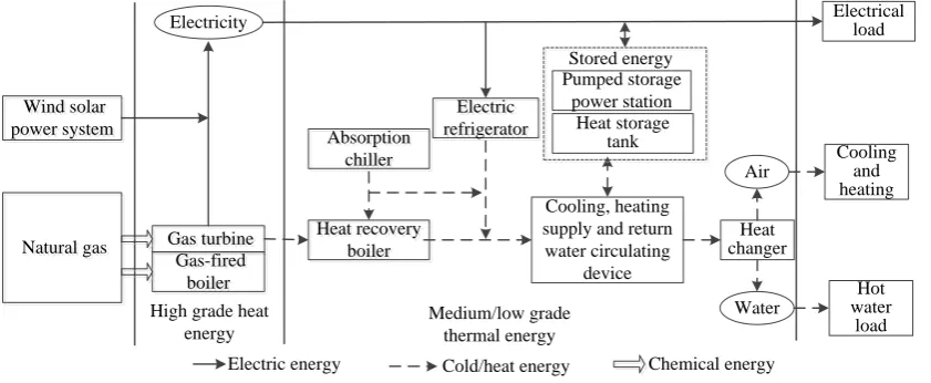
A variety of power generation, cooling and heating equipments are included in the CCHP microgrid. The energy supply structure of CCHP microgrid is shown as Figure 1.
Wind solar power system Wind solar power system Natural gas Natural gas Electricity Gas turbine Gas turbine Gas-fired boiler Gas-fired boiler Absorption chiller Absorption chiller Heat recovery boiler Heat recovery boiler Electric refrigerator Electric refrigerator Pumped storage power station Heat storage tank Cooling, heating supply and return
water circulating device Air Heat changer Water Electrical load Cooling and heating Hot water load High grade heat
energy
Stored energy
Medium/low grade thermal energy
Electric energy Cold/heat energy Chemical energy
Figure 1. Schematic diagram of CCHP microgrid power supply structure
As can be seen from Figure 1, the energy of the entire micro grid can be divided into four parts, including multi-energy supply (source), energy conversion and transmission (transmission), energy storage unit (storage) and terminal energy load (load). Multi-energy supply is a description of microgrid multi-distributed energy output, which generally consists of sustainable power, intermittent power, regional cogeneration of heat and power and primary energy. Energy conversion transmission is an abstraction of various energy conversion characteristics of CCHP microgrid system. According to different forms of energy, there are three types of functional networks: power transmission heat transmission and gas pipe. Energy storage unit is an effective storage and release of energy for load regulation response, which can effectively improve energy utilization efficiency. The terminal energy load is divided into four categories: cooling, heating, electricity and gas. Refrigerator, energy storage and user side power demand are the main forms of power load. Heating load includes hot water, steam, space thermal, etc., which is mainly provided by waste heat recovery unit of micro-turbine, gas boiler and thermal energy storage. Gas load is mainly used to supply gas consumed by gas boilers and micro-turbines. Various loads are the key to regulate energy distribution in micro grid.
2.2 Mathematical model of photovoltaic power generation
When there is no wind, the light intensity is 1KW/m2 and the temperature is 25℃, the relationship among photovoltaic power generation power, light intensity and ambient temperature can be expressed as follows.
[1 ( )]
T
pv pv STC c STC
STC G
P f P k T T
G
= + −
(1)
Where, fpv is a photovoltaic array output power derating factor that takes into account the
power loss of photovoltaic cells due to structural aging and surface covering. Under standard measurement environment, PSTC, GSTC and TSTC are PV output peak power (KWp), light intensity (KW/m2) and temperature (℃), respectively. GT is the actual light intensity of photovoltaic array; k is the temperature coefficient of photovoltaic cell; Tc is the actual temperature of photovoltaic cells, which is jointly determined by environmental temperature and light intensity. The relationship can be expressed as follows.
30 1000
T
c air
G
T =T +
(2)
intensity is greater than 1k W/m2, the peak value will be maintained. When the light intensity is less than 0.4k W/m2, the power generation efficiency will decrease. Based on this, the relationship between photovoltaic cell power generation and light intensity can be obtained.
(0.9 0.1 ) ( ), 0.4
0.4 0.8
), 0.4 1
0.8 , 1 0.8 NTC T T NTC pv T NTC P G G G P
P G G
P G + =
(3)
Where, Ppv is photovoltaic power, and PNTC is the output power of photovoltaic under rated condition. The rated condition refers to wind speed is 1m/s, and light radiation intensity is 0.8kW /m2, and temperature is 20℃.
2.3 Mathematical model of wind power generation
Wind Turbine system is a new clean energy which uses wind turbine (WT) to convert wind energy into electric energy and supply it to users. It is one of the new clean energy with large application potential and fast development. Wind power generation system generally includes wind turbines, speed regulating devices, inverters and controllers. The fan output is affected by the change of wind speed, and the mathematical relationship between them can be expressed as follows.
2 3 1 2
wt p
P = R v C
(4)
Where, Pwt is the generating power of wind turbine; v is the actual wind speed; 𝜌, R are the air
density (kg/m3) and fan wheel blade radius (m), respectively; Cp is the wind energy conversion
efficiency considering turbine loss and transmission loss.
The mathematical relationship between the actual output power and wind speed of a steady-state time-wind unit can be denoted as follows.
3 3 3 3 0, 0 , , 0, in in
r in r
wt r in
r r out
out
v v
v v
P v v v
P v v
P v v v
v v − = −
(5)
Where, Pr and vr are rated power and rated power of the fan respectively, while v, vin and vout
represent the actual wind speed of the fan, the input wind speed and the output wind speed respectively. The wind speed affects the fan's power can be written as follows.
( ) ref ref H v v H
=
(6)
Where Href and vref are the height and wind speed of the measurement point respectively; H is
the height of fan hub; 𝛼 is ground roughness factor.
2.4 Model of pumped storage power station
Pumped Storage (PS), also known as pumped storage hydropower station, is essentially a device for storing and reusing water energy. Pumped storage power generation system is a complex control system of water, machine and electricity. It is consisted of pressure water diversion system, inverter type unit, governor and generator motor, among which reversible type unit has water pump and turbine.
2 1.5
, 1 1 1
,
( )
30
( ) ( 1)
ps ch
ps ch d
P M n D h
E t E t P t
= = − +
(7)
Where, Pps,ch is the accumulative power; M1, n1 and D1are unit shaft, unit speed and runner
diameter of pump turbine respectively. h is the turbine head. E(t) represents the reservoir energy storage after time period t; 𝜂𝑑 refers to the pumped-storage power station pumping efficiency; Δt is pumping time interval.
When the turbine of a storage power station operates under the condition of discharging water, the mathematical relationship between the power converted on the shaft and the reservoir energy storage can be written as follows.
2 1.5
, 1
, 9.18
( ) ( 1) /
ps dis
ps dis g
P QD h
E t E t P t
=
= − +
(8)
Where, Pps,dis is the discharge power; Q= v /t represents the flow velocity. h is the head of the turbine. E(t) represents the upper reservoir energy storage after time period t. 𝜂g is the pumped-storage power station water efficiency. Δ t is water power generation time interval.
2.5 The equipment model of the cooling, heating and power supply system
The mathematical model for generation and heating of the micro-gas turbine used in CCHP system can be calculated as follows.
(1 )
mt mt mt mt
mt mt lost
mt
mt
P V H
P Q = − −
=
(9)
Where, Pmt is the power output of the micro-gas turbine; Qmt is the residual heat of flue gas
discharged simultaneously by the micro-turbine for power generation. Vmt represents the
consumption of fossil fuels (mainly natural gas) per unit of time by the micro-turbine. Hmt refers to
the low calorific value of natural gas, usually 9.78kwh /m3; 𝜂𝑚𝑡 and 𝜂𝑙o𝑠𝑡 are the micro gas turbine power generation efficiency and heat loss coefficient, respectively.
The output of an absorption chiller converting the heat input into heating or cooling can be expressed as follows.
cool cool in
heat heat in
Q COP Q
Q COP Q
=
=
(10)
Where, Qcool and Qheat are the cooling and heat generation power of waste heat absorption
refrigerator, respectively. COPcooland COPheatare the energy efficiency coefficient of refrigeration and
heat energy efficiency of waste heat absorption refrigerator respectively. Qinis the heat input power
of waste heat absorption refrigerator.
The cooling power produced by the compression refrigerator and the electric energy consumed can be expressed as follows.
ec ec ec
Q =COP P
(
11
)
Where,
Q
ecis the refrigeration power of compression refrigerator;
COP
ecrepresents the
refrigeration efficiency coefficient, which is a factor to measure the refrigeration
performance of the compression refrigerator.
P
ecis the power consumed by the compression
refrigerator.
The relationship among the heating power of gas-fired boiler and its output and the amount of natural gas can be expressed as follows.
gb gb gb
Where, Qgb is the heating power of gas-fired boiler; 𝜂gb gas boiler heating energy efficiency coefficient; Fgb is the amount of fuel consumed by a gas-fired boiler.
The dynamic mathematical model of Heat Storage (HS) can be expressed as follows.
( ) ( 1) (1 ) ( ch ch dis/ dis)
hs hs hs hs hs hs hs
E t =E t− −
+ Q
−Q
t(13)
Ehs(t) represents the heat storage state of the regenerator at time t;Qhsch,Qhsdis represent the heat storage power and the heat release power, respectively. hs represents the self-release heat rate of
the equipment. ch hs
, dishs
represent heat storage efficiency and heat release efficiency respectively.3 Load forecasting based on PSO-KELM
The key factors influencing the PV generation and load power were firstly studied to determine the input and output variables of the prediction model. Then particle swarm optimization is used to optimize KELM parameters, and optimized models are used to predict photovoltaic output power and electric load power respectively.
3.1 Influencing factors of PV and load forecasting
Figure. 4 shows the relationship between photovoltaic output power and meteorological factors.
(a)The relationship diagram of photovoltaic power generation and light intensity
(c) The relationship diagram of photovoltaic power generation and relative humidity
(d) The relationship diagram of photovoltaic power generation and wind speed Figure 2. Relationship between photovoltaic power generation and meteorology
Figure 2(a) shows the variation of PV output power and light intensity curves. It can be seen from Figure 2(b) that temperature and PV output power have basically similar variation rules. It can be seen from Figure 2(c) that the PV output curve is basically opposite to the relative humidity curve. FIG. 2(d) shows that there is no correlation between wind speed and PV output change curve. Through the above analysis, it can be known that solar radiation intensity, temperature, weather type and relative humidity affect photovoltaic output power. Daily maximum light radiation intensity, daily maximum temperature, weather type index, daily maximum humidity, and historical PV output power containing PV system information are considered as the input and output variables of the prediction model.
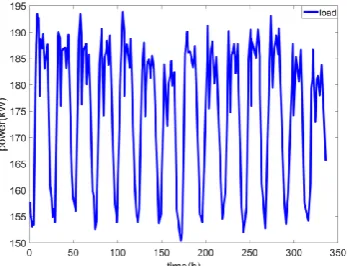
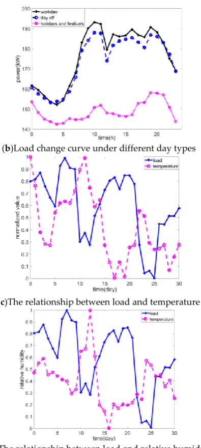
Figure 3 (a) shows the electricity load curve of an area for two consecutive weeks (April 13, 2015 solstice to April 26, 2015). Figure 3(b) shows the load change curve under different day types. Figure 3(c) shows the relationship between average daily load power and average daily temperature in a region. Figure 3(d) shows the relationship between the average daily load power and humidity in a region.
(b)Load change curve under different day types
(c)The relationship between load and temperature
(d)The relationship between load and relative humidity Figure 3. Influence factors of load power
It can be seen from Figure 3(a) that the load has a similar change rule within two weeks, which is reflected by a cycle of 7 days. It can be seen from Figure 3(b) that the load on working days is slightly higher than that on rest days, but the variation trend is similar, while the load on holidays is the lowest, which indicates that different types of days have different influences on load power. As can be seen from Figure 3(c), the average daily load presents an opposite trend to the average daily temperature and humidity.
Through the above analysis on the influencing factors of load prediction, it can be known that the main influencing factors of load power include historical load data, environmental temperature, humidity and day type. Therefore, daily maximum temperature, daily minimum temperature, daily average temperature, daily type index, daily average humidity and historical load power are taken as the input variables of the prediction model.
3.2 Prediction model based on PSO-KELM
3.2.1The mathematic model of ELM
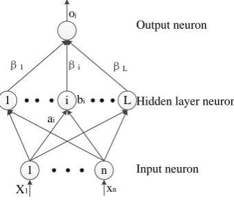
Because only the output weight of hidden layer neurons needs to be calculated, and the hidden layer parameters are randomly obtained, the learning speed of ELM is thousands of times higher than that of traditional BP and support vector machine, etc., and it has better generalization performance. The mathematical model of ELM can be shown in Figure 1.
1 n
1 i L
Output neuron
Hidden layer neuron
Input neuron
X1 xn
ai bi β1 βi βL
oj
Figure 4. The structure of ELM Training set {( , )} 1
N n m
i i i
x t = R R , excitation function g( ) of hidden node is a nonlinear function, which can be selected as Hardlim,Sigmoid, and Gaussian. The number of hidden layer neurons is L.
(1) Hidden layer parameters ( , ),a b ii i =1,..., Lare randomly selected. ai is the input weight of
the hidden layer neuron, and is the threshold value of the hidden layer neuron.
(2) The hidden layer output matrix can be calculated as follows.
1 1 1 1 1
1 1
( ) ( , , ) ( , , )
( ) ( , , ) ( , , )
L L
n n L L n n L
h x g a b x g a b x
H
h x g a b x g a b x
= =
L
M M L M
L
(14)
(3) The output weight can be represented as follows.
¦
(15)
Where is the left pseudo-inverse matrix of the hidden layer output matrix H, and T is the
target output, that is, .
(4) Calculate the output value
O
j. Until the training error is less than the predetermined constant , these training samples can be approached by ELM.1
( , , ), , 1,...,
L
j i i i i j j
i
O g a b x O T j n
=
=
− =(16)
(5) Error calculation.
(
)
2 ( , )1
1
i i
n
a b j j
j=
E
O -T
n
=
(17)
Where, is the hidden layer node weight and threshold,
T
j is the predicted valueIn order to further enhance the generalization ability and stability of ELM, the kernel function is introduced into ELM by comparing the principle of ELM and support vector machine (SVM), and the KELM algorithm is proposed.
(1)The kernel matrix is defined by Mercer's conditions.
, ( ) ( ) ( , )
T ELM
i j j j i j
HH
h x h x K x x
=
= =
(18)
The random matrix HHT of ELM is replaced by nuclear matrix Ω. Using the kernel, all input
samples are mapped from the N-dimensional input space to the high-dimensional hidden layer feature space. When the nuclear parameter setting is completed, nuclear matrix Ω mapping value of
the fixed value. h(x) is the output function of hidden layer node. Kernel K( , )
v is usually set as follows.2
( , ) exp[ ( / )]
K
v = − −
v
(19)
(2)I/C is added to the main diagonal of the unit diagonal matrix HHT so that its characteristic
root is not zero, and then the weight vector
is evaluated.1
( / )
T T
H I C HH T
= + −(
20
)
The output of the KELM model can be expressed as follows.
1 1 1 ( ) ( ) ( / ) ( , ) = ( / ) ( , ) T T ELM Nf x h x H I C HH T
K x x
I C T
K x x
− − = + +
L
(
21
)
The KELM output weight can be expressed as follows .
1
( /I C ELM) T
= + −(
22
)
3.2.2 The mathematic model of PSO
There are n particles in m dimensional space. The position of the ith particle in m-dimensional space can be expressed as xi(xi1,xi2,…xim)[23].The best position experienced by the ith particle is
recorded as pi(pi2,pi2,…pim). The velocity of each particle is defined as vi(vi1,vi2,…vim)[24-25]. The best
place for all particles to pass is written as pg(pi1,pi2,…pim)[26].
After the optimal solution is determined, the particle velocity and position can be updated according to the following equation
1 1 2 2
( 1) ( ) ( (t)) (gbest ( ))
k k k k k k
im im im im im im
v t+ =v t +c r pbest −x +c r −x t
(23)
( 1) ( ) ( 1)
k k k
im im im
x t+ =x t +v t+
(24)
max k( max min) /kmax
= − −
(25)
k im
v is the velocity of particle i in the kth iteration. k im
x is the position of particle i in the kth iteration. k is the current evolutionary algebra. kmaxis the maximum evolutionary algebra, and
isthe weight of inertia. i= 1,2,3... M,is the population size.c1 and c2 are learning factors;. r1 and r2 are random numbers between [0,1]. pbestimk is the position of the individual extremum point of particle
i. gbestkim is the extremum of the whole population. Each particle's speed is limited to [-vmax,+vmax]. The implementation of particle swarm optimization can be described as follows.
Population size N, initial position and velocity vector of each particle, individual extreme value and global optimal solution, iteration error accuracy
, constant coefficients c1 and c2, maximum and minimum inertial values
max and
min, maximum velocity vmax and maximum number of iterations Tmax are set.Step 2: Particalization of the solution of the target problem. The solution of the target problem to be solved is described by the position vector of the particles, and the fitness function of the particles in the particle swarm is determined.
Step 3: The individual extremum of each particle and the global extremum of the population are calculated.
Step 4: Particle velocity and position are updated.
Step 5: Determine whether the following conditions are satisfied. If so, turn to Step 6; otherwise, turn to Step 2.
The iteration error reaches the set precision.
The iteration number of the algorithm reaches the preset maximum iteration number Tmax. Step 6: Output the optimal solution. The particle global optimal value and its corresponding position in the particle swarm are converted into the optimal value and corresponding solution of the target problem, and the algorithm ends.
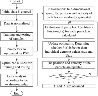
The flow chart of PSO-KELM algorithm can be seen in figure 5.
Start
Initial data is entered Initial data is entered
Data is normalized Data is normalized
Training and testing of samples Training and testing
of samples
Parameters are optimized by PSO
Parameters are optimized by PSO
Optimized KELM for training and testing Optimized KELM for
training and testing
Error analysis according to the evaluation index Error analysis according to the evaluation index
End
Initialization: In n-dimensional space, the position and velocity of
particles are randomly generated Initialization: In n-dimensional space, the position and velocity of
particles are randomly generated
Evaluation of particles: The fitness function f(x) for each particle is
calculated
Evaluation of particles: The fitness function f(x) for each particle is
calculated
Update optimality: Determine whether f (x) is better than individual extreme values pbest and
Gbest
Update optimality: Determine whether f (x) is better than individual extreme values pbest and
Gbest
The position and velocity of the particle are updated The position and velocity of the
particle are updated
Stop judging?
C and λ are obtained
C and λ are obtained Y
N
Figure 5. Flow chart of PSO-KELM algorithm
The regularization coefficient C and the nuclear parameter are optimized by PSO, which have great influence on the accuracy of the prediction model of KELM, then the wind power prediction model is established by PSO-KELM.
The PSO-KELM algorithm flowchart can be represented as follows.
, ,
1 ,
1 n
p i t i
i t i
y y
fitness
n = y
−
=
(26)
Where, yp i, is the original data, yt i, is the predicted value, and fitness is the fitness function
which reflecting the error of model prediction.
The regularization coefficient and kernel parameters of KELM are optimized by PSO to avoid blind training of KELM. In the PSO-KELM prediction model, the output of the KELM learning sample and the root mean square error of the actual output are used as the fitness function of PSO,
the fitness value of the particle is compared with the optimal fitness, and the parameters C and λ of
each KELM are obtained.
The mean relative error is selected as the fitness function of algorithm optimization.
STEP1: The data affecting photovoltaic power generation or load prediction are divided into training set and test set, and the data are normalized.
STEP2: The kernel function of KELM is determined, and RBF kernel is selected, and mapping input vector Xi and initial output weight βint are obtained.
STEP 3 Initialize particle swarm parameters, including population number, particle initial position int and random initial velocity, individual extremum and total extremum;
STEP 4 Particle swarm optimization. According to the objective function, the fitness of each particle is calculated at each iteration, and the speed, position, and global optimal value are updated. The optimal output weight is obtained after iteration.
STEP 5 Calculate the test data output according to the optimal KELM output weight, and the prediction results are obtained according to the evaluation index.
4 CCHP microgrid scheduling model based on MSFLA
4.1 Problem Description
4.1.1Operating cost
The optimal objective function of CCHP is the integrated minimum operation cost.
min f = fom+ fgrid+ ffuel+ fopen
(27)
Where, fom is the cost of operation and maintenance, ffuelis the cost of fuel consumption, fgrid is thecost of power exchange with the grid, and fopenis the cost of opening and closing.
(1) Operation and maintenance cost.
, 1
( ) ( )
N
om om i i
i
f t K P t
=
=
(28)
Where, Kom i, and Pi represent the maintenance coefficient and output size (kW) of the ith
microsource, respectively. (2) Fuel cost.
1 ( ) 1 ( ) N i
fuel ng ng
i i
P t
f t C V C
LHV
=
= =
(29)
Where, V represents the amount of natural gas consumed (m3), Cng refers to the price of natural gas (CNY /m3), LHV represents the low calorific value of natural gas,
i
and Pitand represent the
output of the ith microsource (kW) and the corresponding generation efficiency, respectively. (4) Electric power exchange cost.
( ) ( ), ( ) 0
( )
( ) ( ), ( ) 0
b grid grid
g
s grid grid
C t P t P t
f t
C t P t P t
=
(30)
Where Cb(t) and Cs(t) are the purchase price and sale price (CNY/kW) of the power grid at time
T, respectively. Pgrid(t) is the interaction power (kW) with the grid at time t. Positive value means the
power purchased from the side of the power grid by the micro grid, while negative value means the power sold by the micro grid.
(5) Downtime cost.
, 1
( ) ( ) (1 ( 1))
N
open i i i open
i
f t t t C
=
=
− − (31)
Where,
i( )t and
i(t−1)are the switching state of the ith micro-source (micro-turbine or gasboiler) at the current moment and the previous moment respectively. 1 means turn on, 0 means turn off; Ci open, represents the start-up cost (CNY) of the ith microsource.
Load balance constraint and operation characteristic constraint of each microsource are the main constraints considered in microgrid
(1) Electric load balance.
( ) ( ) ( ) ( ) ( )
Lnet ec mt ps grid
P t +P t =P t +P t +P t
(32)
( )
Lnet
P t ,P tec( ),P tmt( ),P tps( ),Pgrid( )t are net electric load, micro-turbine output, pumped storage output, electric refrigerator power consumption and power exchange with large power grid at time t, respectively. The net electric load is the difference between the total electric load and the wind-solar power, that is, PLnet( )t =P tL( )−PWT( )t −PPV( )t .
(2) Cooling load balance.
, ( ) ( ) ( )
ac cool et c
Q t +Q t =Q t
(33)
Where, Q tc( ) is the cooling load at time t, and Qac cool, ( )t and Q tet( ) are the cooling power of
absorption refrigerator and electric refrigerator at time t, respectively. (3) Thermal load balance.
,
( ) ( ) ( ) ( ) ( )
mt rec ac in gb hs h
Q t
+Q t +Q t +Q t =Q t(34)
( )
mt
Q t ,Qac in, ( )t ,and Qgb( )t are the flue gas waste heat power generated by the micro gas
turbine machine , the heat consumption power of the absorption refrigerator and the heat generation power of the gas boiler at time t. Qhs( )t is the heat storage and release power of the heat storage device at time t. The heat release is positive and the heat storage is negative. Q th( ) is the thermal load at time t;
rec is the conversion efficiency of waste heat recovery unit.(4) Equipment output constraint.
min,i i( ) max,i
P P t P
(35)
min,i
P ,Pmax,i represent the output upper and lower limits of equipment unit i, respectively. (5) Grid interaction power constraint.
min max
grid grid grid
P P P
(36)
Where, min
grid
P and max
grid
P refer to the upper and lower limits of the maximum exchange power between the micro grid system and the large grid, respectively.
(6) Equipment climbing constraints.
( ) ( 1)
( 1) ( )
up
i i i
down
i i i
P t P t P
P t P t P
− −
− −
(37)
(7) Initial and final balance constraint of energy storage.
Cycle continuity of optimized operation of microgrid system and time of energy storage unit (pumped storage, heat storage tank).
When segment coupling is considered, the initial and final energy storage of multi-period periodic scheduling needs to be consistent.
0 end
E =E
(38)
Where, E0 and Eend are energy storage at the beginning and end of cycle scheduling of energy
storage devices, respectively.
4.1.2 Constraint processing method
min, max,
max( , ( 1) down) ( ) min( , ( 1) up)
i i i i i i i
P P t− −P P t P P t− +P
(39)
The equipment output update needs to be satisfied with Equation (40). When the constraint is not satisfied, the formula is adjusted as follows:
min, min,
max, max,
max( , ( 1) ), ( ) max( , ( 1) ) ( )
min( , ( 1) ), ( ) min( , ( 1) )
down down
i i i i i i i
i up up
i i i i i i i
P P t P P t P P t P
P t
P P t P P t P P t P
− − − −
= − + − +
(40)
Where, P ti( ) and P ti( −1) represent the output of the ith equipment unit at the current
moment and the previous moment, respectively. up i
P and down i
P represent the maximum increased power output and maximum decreased power output of equipment unit i in time period t. Micro gas turbine and gas boiler are mainly considered as equipment with climbing constraints in this paper.
For the equipment without climbing constraint, but constrained by the output upper and lower limits, the formula is adjusted as follows.
min, min, min max, max, max, , ( ) ( ) ( ), ( ) , ( )
i i i
i i i i
i i i
P P t P
P t P t P P t P
P P t P
=
(41)
Considering the new objective function of energy storage constraints, take pumped storage power station as an example.
0
min fnew= +f E −Eend
(42)
After the initial and final balance of the reservoir energy storage state in a pumped storage station is considered, the above equation can be modified as follows.
, ,
1 1
min /
T T
new d t d g t g
t t
f f
P
P
= =
= +
−
(43)
Where, Pd t, and Pg t, are the storage discharge power of pumped storage power station in time period t.
d and
g represent the storage discharge efficiency of pumped storage station,respectively.
4.2 Shuffled Frog Leaping Algorithm
Inspired by Shuffled Frog group Leaping and foraging behavior, a new Shuffled Frog Algorithm (SFLA) was proposed. SFLA's mathematical model can be described as follows.
Assuming that the problem to be solved is a D dimensional vector, the initial P frogs are randomly generated within the feasible threshold. The location of the ith frog can be represented as
1 2
{ , ,..., }
i i i iD
x = x x x , the fitness function value of each individual is calculated and arranged in descending order according to size, the optimal fitness value of the current population is selected, and the corresponding individual xg is recorded. Then the population is divided into M
subpopulation groups, each subpopulation contains N individuals, that is, P=M×N, the rules of division is that the first frog is assigned to the first subgroup, the second is assigned to the second subgroup... The M frog is assigned to the M subgroup, the M+1 is assigned to the first subgroup, and so on until all the individuals were divided.
Local search: The individuals with the best and worst adaptive values of each subpopulation are denoted as xband xw respectively. At each iteration of the loop, the worst individual is updated in
position. The update policy formula can be expressed as follows.
( 1) () ( )
( 1) ( ) ( 1)
i b w
w w i
D t rand x x
x t x t D t
+ = −
+ = + +
Where, Di[Dmin,Dmax] is the update step size for each jump, and rand() is the randomly generated number within the range of [0,1]. x tw( +1) is the updated position of the individual.
Global search: after a fixed number of local searches are completed, all subpopulations are
remixed into a single population so that the various group information can be communicated
to each other. In descending order of fitness, the subgroups are regrouped, and local searches
continue until the termination condition is met.
4.2.1 Flow of SFLA
The implementation process of SFLA is generally divided into four steps: initialization, population grouping, local search within cluster group, and cluster group remixing. The specific process can be described as follows[27].
(1) Relevant parameters to initialize the population are input.
(2) Sorting: According to the characteristics of solving the problem, the fitness value of each frog in the population was calculated, and all the individuals were sorted according to the fitness value.
(3) Grouping: The population was divided into M subgroups according to the fitness value. Each subgroup contained N frogs. The optimal individual and the worst individual in each subgroup were recorded respectively.
(4) Subgroup local search: the worst individual in the subgroup is updated according to formula (44), and the subgroup and the global optimal individual are also updated.
(5) Judge whether the local search of subgroup reaches the maximum number of iterations, if not, jump to (4) to continue execution.
(6) Subgroup remixing: all subpopulations are mixed into one population, all individuals are arranged according to fitness value, and the global optimal individual information is updated.
(7) Whether the global maximum number of evolutionary iterations or convergence accuracy meets the requirements; if so, exit the algorithm; otherwise, return back to (3).
4.2.2 Improved Shuffled Frog Leaping Algorithm (MSFLA)
(1) Cauchy mutation operator
Cauchy distribution is a kind of functional distribution commonly used in mathematical statistics and other fields. Its probability density distribution function can be written as follows[28-30].
2 2
( ) ,
( ( ) )
f x x
x
= −
+ −
(45)
Where, when =0, =1 is satisfied, it is called the standard cauchy distribution, denoted by C(0,1).
When the traditional SFLA is iterated for many times, new individuals in the subgroup may fall into premature convergence. The variation of random Numbers obeying Cauchy distribution will produce large update step, which is helpful for the population to jump out of local extremum. In this way, the optimization performance in the larger solution space is better and the global searching ability of the algorithm is improved. The improved local update strategy can be written as follows.
( 1) () ( ) (0,1)
( 1) ( ) ( 1)
i b w
w w i
D t rand x x C
x t x t D t
+ = −
+ = + +
(46)
(2) Adaptive variation.
The idea of adaptive mutation is introduced into SFLA and can be expressed as follows.
2 1 2 max 2 ( ) ( ( )) , ( ) , ( ) avg i i avg avg m i avg
k k f f x
k f x f
f f
p
k f x f
When the fitness value of an individual is better than the average fitness value, a lower mutation probability is assigned to protect the individual to enter the next iteration. On the contrary, if the fitness value of an individual is less than the average fitness value, the corresponding mutation probability is higher, and the individual can be eliminated.
(3) Disturbance operation.
If the diversity of the population is guaranteed, the global search capability is improved, and the individual updates are followed by another disturbance operation, which can be expressed as follows.
, ,
(max( ) min( )) / 2
( ) ( ) 2 ()
j j
i j i j
r x x
x t x t r rand r
= −
= + −
(48)
Where, r is the disturbance radius; xjis the jth dimension value of the population individual, xi,j
is the jth dimension value of the ith individual of the population.
4.3 MSFLA based CCHP microgrid scheduling model
With the day-ahead economic minimization cost of CCHP as the objective function, the scheduling model was solved by MSFLA. The steps for optimal operation of the micro-grid can be expressed as follows.
(1) Input data is read and initialized. Micro grid system and output limit to the number in various kinds of micro power supply, power system load demand, wind power and photovoltaic power generation forecasting data, each unit of initial state parameters (pumped storage reservoir storage state, micro gas turbine power generation, thermal energy storage condition, etc.), energy price information (time-sharing electricity, natural gas price), equipment performance parameter information, determine the scheduling to the total number of time T, set MSFLA parameters (child/total group scale, the number of iterations and mutation probability constant) are included.
(2) The population is randomly initialized. According to the output limitation of each micro-source equipment, micro-turbine, pumped storage, heat storage tank and gas boiler are selected as decision variables, and the initial population individuals are randomly generated in the feasible region, and their positions are represented as a group of feasible scheduling plans. The output of the electric refrigerator, the output of the absorption refrigerator and the heat recovery power of waste heat can be determined by the balance constraint of the cold and heat power and the calculation of the decision variables. The interaction power with the grid can be calculated by load balancing constraints and decision variables. Fuel consumption, gas waste heat power of micro gas turbine and power consumption of refrigeration equipment can be calculated according to corresponding mathematical model and energy conversion coefficient.
(3) Individuals of the population are modified by constraints. The individuals in the population who violate the constraints are adjusted, the decision variables are adjusted back to the feasible solution space, and the adjusted population is obtained.
Equation (30) is used as the fitness function of algorithm optimization. Fitness values were calculated for each individual, and then all individuals were ranked in descending order according to fitness values.
(5) According to the fitness value, the population was divided into M groups, each group containing N frogs, and the optimal and worst individuals in each subgroup were recorded respectively.
(6) The worst individual in each subgroup is updated according to Equation (47). According to formula (44), individuals are subjected to mutation operations. If the fitness value of the individual after variation is better than that before, the replacement is carried out. Simultaneously the clipboard is updated (subgroup and globally optimal individual).
(8) All subpopulations are mixed into one population, and all individuals are rearranged according to fitness value to update the global optimal individual information.
(9) Check whether the global maximum number of evolutionary iterations or convergence accuracy meets the requirements, and if so, jump to the next step. Otherwise, skip step (5).
(10) Global optimal value and corresponding decision variable value are output, output of each micro-source equipment is solved, and optimal scheduling scheme is obtained.
5 Simulation
5.1 Photovoltaic power generation forecast
The radial basis function (RBF) is selected, and setσ=0.1, C=0.5. The number of PSO population
is set as 25, the initial output weight calculated by KELM is set as the initial position of the particle, the initial velocity of the particle is randomly selected in [0,1], and the particle dimension is the output weight dimension. Table 1 shows the evaluation indexes of the predicted results under different weather conditions including KELM, GA-KELM and PSO-KELM.
Table 1 Models’ prediction and evaluation of different weather conditions
Prediction
algorithm
Sunny Cloudy Runny
RMSE MAPE RMSE MAPE RMSE MAPE
KELM 0.17631 0.1011 0.60119 0.3328 0.29756 4.2544 GA-KELM 0.16517 0.0535 0.52726 0.1822 0.29564 3.7162 PSO-KELM 0.16376 0.0376 0.48986 0.1649 0.24274 3.714
Figure 6 shows the comparison curve between the predicted value and the real value of photovoltaic output power under different prediction models in sunny days. In order to show the photovoltaic power generation prediction results of the three models, the relative error comparison between the predicted value and the true value is shown in Figure 7.
Figure 6. Photovoltaic power generation prediction results under different prediction models
It can be seen from Figure 6 that the photovoltaic prediction results of the three models are generally consistent with the actual values. However, the photovolatic prediction curve of GA-KELM in sunny days is superior to that of traditional KELM. In the three models, the predicted value of PSO-KELM is closer to the true value. It can be seen from Figure 7 that the prediction error of PSO-KELM is less than GA-KELM and KELM.
5.2 Power prediction of electric load
The historical electric load power, the corresponding meteorological information and the day type, calculated from March to May, 2015, are selected as the training and prediction model. The electric load power is selected from 0:00 to 23:00, and the time interval is 1h. According to the above analysis of affecting factors of load forecasting, load power, the day before the same time the day before the highest temperature, the lowest average temperature, average temperature, humidity, type index, two days before the load power at the same time, predict daily maximum temperature, minimum temperature, average temperature, average humidity and day type index are used as the prediction model of input; The output variable is the load power at the corresponding time of the predicted day.
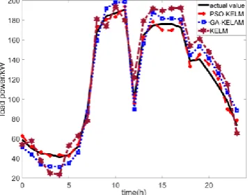
Figure 8 shows the prediction results of KELM, GA-KELM and PSO-KELM on the working-day. Figure 9 shows the relative error curves of the three prediction models for the load power prediction results.
Figure 8. Comparison curve of load power prediction
Figure 9. Comparison curve of relative error of load prediction power
As can be seen from Figure 8, PSO-KELM load forecasting results are more accurate than GA-KELM and KELM, improving the global search capability. The reliability of the proposed method is verified.
As can be seen from Figure 9, PSO-KELM prediction method has the smallest relative error at most times of a day, while KELM prediction model has the largest relative error. Therefore, PSO-KELM is a relatively better prediction model, with smaller relative error and higher accuracy.
the difference in electrical load demand of different day types, PSO-KELM, GA-KELM and KELM were also used to predict the load of different day types such as weekends and holidays. Table 3 shows the load forecasting results for different day types.
Table 2 Prediction results of the three prediction models in working days Prediction
algorithm
MAPE RMSE MAE CC
KELM 0.0285 8.2432 6.9744 0.9943
GA-KELM 0.0189 5.3517 4.4157 0.9974
PSO-KELM 0.0115 3.6756 2.6398 0.9981
Table 3 Prediction performance evaluation of different day types by the three models Prediction
algorithm
Weekends May day holiday
MAPE RMSE MAE CC MAPE RMSE MAE CC
KELM 0.021 4.6258 3.5368 0.9852 0.0819 12.9458 12.1041 0.9479 GA-KELM 0.0197 4.6237 3.2549 0.9855 0.0632 10.5152 9.2097 0.9588 PSO-KELM 0.0192 4.5407 3.1737 0.9857 0.0506 9.1065 7.2219 0.9631
As can be seen from the table 1, PSO-KELM has the best prediction effect and the highest accuracy. The reliability of the proposed PSO-KELM algorithm is verified.
As can be seen from Table 3, Among the three prediction models, PSO-KELM has the best prediction effect for different day types, while KELM has the worst prediction accuracy. At the same time, it can be seen that different forecasting models have a good effect on the load forecasting of weekends and rest days, and a relatively poor accuracy on the Load forecasting of May day holidays. The main reason is that the electrical load on the rest day is similar to that on the working day and has its periodic change rule. On the one hand, holiday load is affected by various uncertain factors, such as human activities, and its variation regularity is poor. On the other hand, it is caused by the lack of data collection for this type in training samples and the insufficient extraction of sample characteristic values by the prediction model.
5.3 Performance test of MSFLA
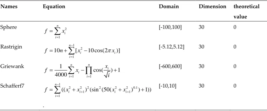
In order to verify the performance of the proposed MSFLA, four test functions are selected for simulation verification.
Table 4 Standard test functions
Names Equation Domain Dimension theoretical
value
Sphere 2
1 n i i f x =
=
[-100,100] 30 0Rastrigin 1
2
1
10 [ 10 cos(2 )]
n
i i
i
f n x x
−
=
= +
− [-5.12,5.12] 30 0Griewank
1 1
1
cos( ) 1 4000 n n i i i i x f x i = =
=
− + [-600,600] 30 0Schafferf7 1
2 2 2 2 2 2 0.1
1 1
1
(( ) (sin (50( ) ) 1))
n
i i i i
i
f x x x x
−
+ +
=
=
+ + +.
[-10,10] 30 0
PSO is w1 =0.9, w2 =0.4, and the learning factor is c1 = c2 =2. In order to reduce the random error in the simulation process and test the performance of the algorithm, the search times of each group of test functions are set as 20, and the average value of the operation results is taken. The simulation results are shown in Figure 10 and Table 5.
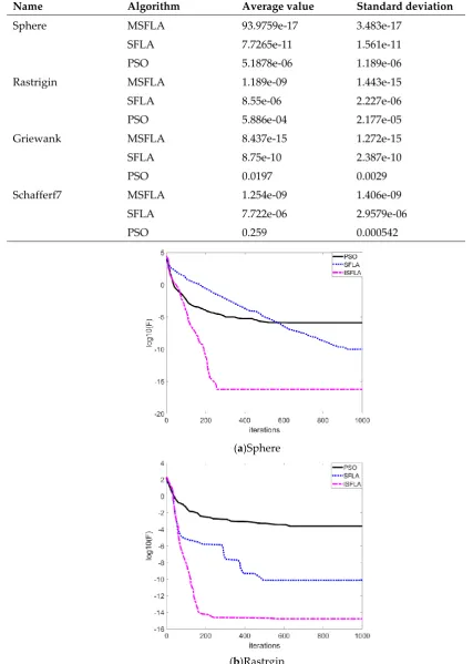
Table 5 Comparison of simulation results of three algorithms
Name Algorithm Average value Standard deviation
Sphere MSFLA 93.9759e-17 3.483e-17
SFLA 7.7265e-11 1.561e-11
PSO 5.1878e-06 1.189e-06
Rastrigin MSFLA 1.189e-09 1.443e-15
SFLA 8.55e-06 2.227e-06
PSO 5.886e-04 2.177e-05
Griewank MSFLA 8.437e-15 1.272e-15
SFLA 8.75e-10 2.387e-10
PSO 0.0197 0.0029
Schafferf7 MSFLA 1.254e-09 1.406e-09
SFLA 7.722e-06 2.9579e-06
PSO 0.259 0.000542
(a)Sphere
(c)Griewank
(d)Schafferf7
Figure 10. Optimization curves of the test functions
It can be seen from Figure 10 and Table 4 that the optimization results presented by the three algorithms are different. MSFLA is superior to SFLA and PSO in terms of average optimal value, optimal solution and standard deviation, which indicates that improved SFLA has higher optimization precision and better algorithm stability.
5.4 Comprehensive energy optimization scheduling based on PSO-KELM and MSFLA
In this paper, it is assumed that the rated power of the micro gas turbine (MT) is 100kW, the power generation efficiency is 0.4, the heat dissipation coefficient is 0.1. The equipment climbing and descending amount is 80kW, and the start-stop cost is 5 CNY. The total capacity of the pumped storage power station (PS) reservoir is 350kW. The maximum charge-discharge power is 50kW. The charge-discharge efficiency is 0.95, and the self-loss rate is 0.0025. Heat storage tank (HS) capacity is set to 300kW. Maximum heat storage and release power is 50kW. Heat storage efficiency is 0.8, and heat release efficiency is 0.9. Self-loss rate is set to 0.003. Absorption refrigerator (AC) refrigeration coefficient is 1.2, and heating coefficient is 0.8. The refrigeration coefficient of electric refrigerator (EC) is 4.3, and the maximum refrigeration power is 150kW. The maximum heat generation power of gas-fired boiler (GB) is 300kW, and the heat generation coefficient is 0.95. The climbing and descending amount of equipment is 100kW, and the start-stop cost is 5 yuan. The number of optimized cycles is T=24.
Table 6 Maintenance coefficient of equipment operation
Equipment PS GB MT HS AC EC
Maintenance cost(CNY/kWh)
0.005 0.04 0.06 0.001 0.008 0.0097
Table 7 Information table on energy prices
Time price of power
purchase(CNY/kWh)
price of sell
electricity(CNY/kWh)
price of natural
gas(CNY/m3)
Valley period 0.443 0.31 2.05
Flat period 0.66 0.506 2.05
Peak period 1.314 0.92 2.05
Due to the difference in load demand of cold, heat and electricity in summer and winter, there are different requirements for optimal dispatching of CCHP micro-grid. The typical days in summer and winter are analysed respectively. The proposed PSO-KELM algorithm is used to predict the cooling, heating and wind power in the short term. Figure 11 shows the forecast data of cooling, heating and electric load demand in two typical days in summer and winter, and Figure 12 shows the predicted power change curves of wind power generation and photovoltaic power generation in summer and winter.
(a)Typical load demand in summer
(b)Typical daily load demand in winter
(a)Typical solar power generation in summer
(b)Typical solar power in winter
Figure 12. The predicted power curve of wind-solar power generation in a typical day in summer and winter
5.4.1 Simulation of typical daily optimal scheduling in summer
In summer, the optimized scheduling results of cooling, heating and electricity loads are shown in Figure 13, Figure 14 and Figure 15, respectively.
Figure 14. Typical diurnal cold equilibrium curve in summer
Figure 15. Typical daily heat balance curve in summer
It can be seen from the electric load balance dispatching curve in Figure 13 that, in order to make full use of wind power and photovoltaic power generation, new energy is absorbed to the maximum extent. Net electric load refers to the difference between the predicted electric load and the wind output at the corresponding time.
From 23:00 to 7:59 in the valley period, power is purchased from the large grid to drive the air conditioning refrigerator for refrigeration to meet the cooling load demand. The peer pumped the energy to store the electricity in the valley period and transfer it to the peak period for utilization. At the end of the 7th period, the pumped storage power station reaches the maximum energy storage state.
During peak hours of 8:00-13:59 and 18:00-20:59, the side purchase price of power grid is relatively high. The pumped storage power station operates with maximum output, and the remaining power shortage is made up by the micro-turbine. In this period, the power generation cost of the micro-gas turbine is less than the electricity selling cost of the grid. Therefore, when the pumped storage energy and the micro-gas turbine jointly generate electricity to meet the system's electrical load demand, the micro-gas turbine runs at full capacity and sells the remaining electricity to the external network to earn profits. The pumped storage station discharges at the end of 13:00 and 20:00, and the reservoir energy storage reaches the lower limit.
During the peacetime period from 14:00 to 18:59, the gas-fired generator works at full capacity to meet the electrical load demand of the system, and the insufficient part purchases electricity from the grid. At the same time, in this stage, the maximum charging power is used for pumping and storing electricity to prepare energy storage for discharging in the next peak period.
power supply cost in peak period is reduced, and the overall economy of the micro-grid system is improved.
Figure 14 and Figure 15 are used to analyse the cold and heat energy balance of the cold-heat and power supply micro-grid. In summer, the demand for cooling load is strong, while the demand for heating load is relatively small. In the period of low electricity price, the cooling load of the system is satisfied by electric refrigeration and air conditioning, and the hot load is satisfied by micro-gas turbine generating power, without gas boiler output. In peacetime period from 14:00 to 18:59, the cooling capacity of electric refrigeration air conditioning increased. The flue gas waste heat generated by the micro-turbine in ordinary times is stored by the heat storage device and released and utilized in the evening peak period to reduce the comprehensive economic cost of the system. At 23:00 in the valley, due to the decrease of cold and hot loads and the influence of off-peak electricity price, the micro-turbine is in the state of shutdown. The cooling load is satisfied by the refrigeration air conditioning, and the hot water load is balanced by the heat release of the heat storage device.
Figure16 shows the change curve of the energy storage state of reservoirs in pumped storage power stations. The operating costs of the cooling, heating and power co-supply microgrid system are calculated and compared with the cost of the traditional co-supply microgrid system. The results are shown in Table 8 and Figure 17.
Figure 16. Change curve of reservoir energy storage state in pumped storage power station
Table 8 Comparison of operating cost between cold, heat and power supply and power supply Energy method fom(CNY) ffuel(CNY) fgrid(CNY) fopen(CNY) total(CNY)
Combined supply of cooling
121.47 1359.67 208.91 10 1700.05