1 Article
1
Energy Management through Cost Forecasting for
2
Residential Buildings in New Zealand
3
Linlin Zhao 1, Zhansheng Liu 1,*, and Jasper Mbachu 2
4
1 College of Architecture and Civil Engineering, Beijing University of Technology, Beijing 100124, China;
5
llzhao@bjut.edu.cn
6
2 Faculty of Society & Design, Bond University, Gold Coast 4226, Australia; jmbachu@bond.edu.au
7
* Correspondence: liuzhansheng@bjut.edu.cn
8
9
Abstract: Over the last two decades, residential buildings have accounted for nearly 50 percent of
10
total energy use in New Zealand. In order to reduce household energy use, the factors that influence
11
energy use should be continuously monitored and managed. Building researchers and professionals
12
have made efforts to investigate the factors that affect energy use. However, few have concentrated
13
on the association between household energy use and the cost of residential buildings. This study
14
examined the correlation between household energy use and residential building cost. Analysis of
15
the correlation between energy use data and residential building cost indicated that residential
16
building cost in the construction phase and energy use in the operation stage were significantly
17
correlated. These findings suggest that correct monitoring of building costs can help to identify
18
trends in energy use. Therefore, this study proposes a time series model for forecasting residential
19
building costs of five categories of residential building (one-story house, two-story house,
20
townhouse, apartment, retirement village) in New Zealand. The primary contribution of this paper
21
is the identification of the close correlation between household energy use and residential building
22
costs and provide a new area for optimize energy management.
23
Keywords: residential energy use; energy management; residential building costs; exponential
24
smoothing method; ARIMA model
25
26
1. Introduction
27
Energy consumption in the residential sector is increasing due to rapid urbanization and social
28
development. The residential sector consumed 45% of the nation’s energy. The expansion of
29
residential areas contributes significantly to the increase in energy consumption and CO2 emission,
30
resulting in global warming and air pollution. The existing literature indicates that the efficiency of
31
end-use energy can significantly reduce total global energy consumption [1, 2]. Proper management
32
of household energy use plays a key role in the management of energy demand. Knowledge of the
33
factors that affect energy consumption is essential for proper energy management. To improve
34
energy efficiency in the residential sector, decision-makers must continuously monitor and manage
35
the factors that influence energy use in the residential sector. Several previous studies focused on
36
factors that influence energy efficiency, including climate [3], time periods [4], environmental and
37
economic impacts [5], building features [6], procurement process [7], building envelopes [8], heating,
38
ventilation, and air conditioning (HVAC) [9], indoor temperatures [10], smart lighting and appliances
39
[11] and occupant behavior [12]. However, only a limited number of studies examined the
40
relationship between energy use and building costs. This study investigates the association between
41
residential building cost and energy use in residential buildings.
Electricity, gas, and petrol are types of energy that are integral parts of human life. The
44
residential sector is the greatest energy consumer. A significant amount of energy is used to provide
45
comfortable indoor environments. Since the demands of all users should be satisfied, understanding
46
to future trends of energy use has become important. It is important for energy demand side
47
management to know the future trends of electricity and gas consumption in the residential sector.
48
Prediction of the factors that influence household energy use is essential for continuous monitoring
49
and management of energy consumption. Residential building costs are estimated in this study to
50
properly manage household energy use since the study hypothesizes that residential building cost is
51
significantly correlated with household energy use.
52
Given the utmost importance of cost forecasting and the important role of predicting it
53
accurately, this study tends to use time series modelling techniques to forecast the building cost of
54
five categories of residential building including one-story house (AR1), two-story house(AR2),
55
townhouse (AR3), apartment (AR4), retirement village (AR5) in New Zealand. Building costs time
56
series usually exhibit strong trends presenting challenges in developing useful models. How to
57
effectively model building cost series and how to enhance forecasting performance are still
58
outstanding questions. There are two most widely used time series forecasting methods: exponential
59
smoothing and Autoregressive Integrated Moving Average (ARIMA). The performance of the two
60
forecasting techniques was evaluated in terms of error measures.
61
Exponential smoothing method was originally introduced by [13, 14]; for short-term sales
62
forecasting in support of supply chain management and production planning. The widespread usage
63
of this method is mainly due to the fact that it is a relatively simple forecasting method requiring a
64
small size sample and having a comprehensible statistical framework and model parameters.
65
Exponential smoothing models developed are based on the trend and seasonality in time series, while
66
ARIMA models are supposed to describe the autocorrelations in the time series. A framework for
67
exponential smoothing methods was developed based on state-space models [15].
68
Autoregressive Integrated Moving Average (ARIMA) approach is a renowned and widely used
69
linear method [16]. It carries more flexibility by representing various components of time series
70
including autoregressive (AR), moving average (MA), and combined AR and MA. It is the most
71
efficient approach for short-term forecasting with rapid changes. ARIMA models can also predict the
72
future based on modelling the behavior of the serial correlation between the observations of the time
73
series. The future predictions based on ARIMA models can be explained by previous or lagged values
74
and the terms of the stochastic errors [17].
75
Time series forecasting techniques such as exponential smoothing models and the ARIMA
76
models have not yet been examined for residential building cost forecasting in New Zealand.
77
Therefore, the study as original contribution to the existing literature is for the first time to evaluate
78
the forecasting performance of these models for residential building cost in New Zealand. Moreover,
79
based on the comparison of the forecasting techniques, industry practitioners can derive a general
80
understanding of forecasting techniques for building cost, and thereby improve forecasting accuracy.
81
The rest of this study is organized as follows. Section 2 presents the previous studies about
82
factors influencing residential energy use and cost forecasting methods. Section 3 introduces
83
correlation analysis, exponential smoothing method, and ARIMA models. Correlation analysis
84
results, exponential smoothening and ARIMA models for the cost series are shown in Section 4. In
85
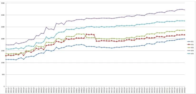
Section 5, the comparison of cost models based on error measures is described. Results discussion is
86
presented in Section 6. In the final section, conclusion is presented.
87
2. Literature Review
88
2.1. Influencing Factors of Residential Energy Use
89
Increased use of energy has already raised concern about exceeding supply capacities and severe
90
environmental impacts, including global warming and climate change [18]. The residential sector
91
significantly contributes to energy consumption, such as electricity, gas, and petrol. Many factors
influence household energy use, including weather, building design, energy systems, and
socio-93
economic factors. Several studies have been conducted that focused on the investigation of the factors
94
that influence energy efficiency.
95
A previous study explored the relationship between energy use and indoor thermal comfort
96
[19], indicated that weather and climate have significant effects on household energy use. For
97
example, in cold regions, people need more electricity or gas to warm up their houses. Recently, due
98
to the increased demand for sustainable development more studies focused on how to improve
99
energy efficiency. For example, some study stated that building features such as orientation can
100
impact energy use by the proper use of natural resources, including sun light and natural ventilation
101
[20]. Energy efficiency can be improved by using public-private partnership (PPP) practices [21, 22].
102
Certain financial and technological hints were used to manage energy that improved energy
103
efficiency. Another study stated that certain innovative technologies can be incorporated into the
104
project delivery process for reducing energy consumption [23, 24]. In addition, other studies explored
105
the use of an evolved HVAC system and an advanced building envelope can improve energy
106
efficiency in the operation stage [25-27]. For example, the smart lighting system can improve energy
107
performance in a building [28]. Moreover, effective implementation of home appliances improve
108
energy efficiency [29].
109
2.2. Cost Forecasting Methods
110
The main issue is forecasting building cost simply and accurately. For example, [30] developed
111
a simple model to predict total project cost taking into account the effect of economic inflation. [31]
112
illustrated a suitable method for examining cost overruns by involving political influences, and
113
delays and economic inflation, during the project process. [32] introduced a mathematical model for
114
investigating the accuracy of early cost estimates by using principal component analysis and
115
regression analysis. [33] presented a probabilistic model based on the Poisson process for estimating
116
project cost contingencies. [34] proposed an integrated regression model by including the strengths
117
of probabilistic and parametric techniques to estimate conceptual cost. [35] categorized the leading
118
cost drivers to evaluate future total project cost.
119
Although these methods are effective in identifying the leading cost drivers and appropriate
120
estimation at the inception of the project, they are difficult to deal with as time-varying variables and
121
reflect the time lag effects. Since much time-related data are dependent or have an autocorrelation
122
[36], time-related techniques can be adopted to overcome these limitations.
123
2.3. Time Series Models for Cost Forecasting
124
In an attempt to solve time-related problems in the methods, time series techniques, which
125
estimate future values of a certain variable according to past values of itself and random shock
126
factors, have been adapted to cost forecasting in construction projects. For example, [37] used
time-127
series models to provide reliable forecasts of building costs, tender prices, and the impacts of
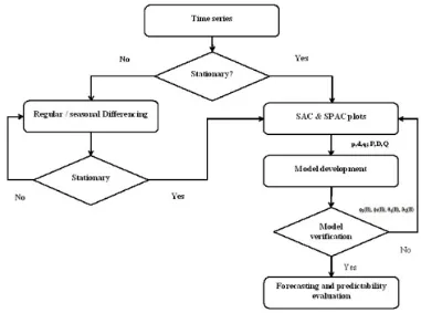
128
economic inflation on building projects. Moreover, [38] explained a way of applying neutral networks
129
to forecast changes in the construction cost index. [39] suggested a time-series approach to identify
130
the leading factors causing escalated construction cost. [40] introduced an integrated regression
131
analysis and ARIMA techniques to predict a tender price index for Hong Kong building projects. [41]
132
developed a Box-Jenkins model to estimate the labor market of the Hong Kong construction industry.
133
[42] addressed a dynamic regression model to examine the relationship between the economic
134
conditions in the market and construction cost. [43] illustrated a time series method that estimates
135
future values according to past values and corresponding random errors and produces a reliable
136
prediction of construction cost. These time series techniques provide systematic and time-related
137
models to forecast future values. According to [41], it is possible to make accurate predications based
138
on historical patterns.
139
141
3. Research Methods
142
3.1. Data
143
The building cost index is useful for construction professionals to quantify cost variations [44].
144
The index can provide information of cost changes caused by a combination of changes in material,
145
labor, and equipment. Hence, the cost index has been used widely in the industry for cost estimation
146
[43]. The cost index provided by QV cost-builder have been accepted in the Architecture, Engineering
147
and Construction (AEC) industry in New Zealand. QV cost-builder carried out various surveys on
148
construction economics including construction material, labor, and equipment costs to provide
149
comprehensive statistical information. As for many other industries and sectors, QV cost-builder
150
compiles historical data to guide construction organizations and industry professionals and to
151
identify cost fluctuations in the construction industry. The cost forecasting application undertaken in
152
this study is based on the average quarterly building cost data for the five categories of residential
153
building in New Zealand. The variables of residential energy use include household electricity use,
154
household gas use, and household petrol use. The energy variables are obtained from Statistics New
155
Zealand which compiles historical data of household energy use.
156
The available dataset consists of quarterly data over a period of 18 years (72 observations) for
157
three types of household energy use and five categories of residential building costs in New Zealand.
158
The cost data are separated into two sections: in-sample data and out-of-sample data. The in-sample
159
data are used for model fitting and the out-of-sample data aims to evaluate the forecasting
160
performance of the model [45]. The data (72 observations) was split into two parts: the training part
161
for model fitting and the testing part for evaluating forecasting performance by comparing forecasts
162
with observations [46]. There is no clear rule for this dividing; in this study, about 72% of the data
163
(2001:Q1-2013:Q4) were used for model fitting and the remaining 28% (2014:Q1-2018:Q4) were used
164
for out-of-sample forecasts evaluation. The quarterly average building cost for the five categories of
165
residential building in New Zealand from 2001:Q1-2018:Q4 are depicted in Figure 1.
166
167
168
169
Figure 1. Building cost time series for five categories of residential building in New Zealand
170
171
173
3.2. Correlation Analysis
174
Correlation analysis is a statistical method used to evaluate the significance of correlation
175
between two variables [47]. A significant correlation indicates that two variables have a significant
176
relationship, while a weak correlation indicates that the variables are weakly related. In other words,
177
correlation analysis can be used to examine the significance of the relationship between two variables.
178
Pearson’s correlation coefficient, also called linear correlation coefficient, assesses the linear
179
relationship between two variables [48]. Let i and j be two random variables of the same sample n.
180
To calculate Pearson’s correlation coefficient r, use Equation (1) as follows:
181
182
𝑟 = ∑𝑛𝑘=1(𝑖𝑘−𝑖̂)(𝑗𝑘−𝑗̂)
√∑𝑛𝑘=1(𝑖𝑘−𝑖̂)2√∑𝑛𝑘=1(𝑗𝑘−𝑗̂)2
, (1)
Where
183
𝑖̂ =1
𝑛∑ 𝑖𝑘 𝑎𝑛𝑑 𝑗̂ = 1
𝑛∑ 𝑗𝑘 𝑛 𝑘=1 𝑛
𝑘=1 ,
are the means of the variables i and j, respectively. The correlation coefficient r ranges between
184
-1 and +1. If the linear correlation between i and j is positive (the increase of one variable is related to
185
the increase of the other), then the correlation coefficient r >0, whereas if the linear correlation
186
between i and j is negative (the increase of one variable is related to the decrease of the other), then
187
the correlation result r <0. The value r = 0 indicates absence of any association between i and j. The
188
sign of the correlation coefficient indicates the direction of the relationship. The magnitude of r
189
indicates the significance of the correlation. For example, if r is close to 1, then the two variables are
190
positively associated at a significant level, which also indicates that the increase of one variable is
191
related to the increase of the other. If r is close to -1, then the two variables are negatively associated
192
with each other at a significant level, which indicates that the increase of one variable is related to the
193
decrease of the other. If r = 0, this usually indicates the two variables are unrelated.
194
3.3. Exponential Smoothing
195
Exponential smoothing is one of the most effective forecasting methods when a time series has
196
a trend that has changed over time, for example, since the 1950s [49]. It unequally weights the
197
observed time series values. More recently observed values are weighted more heavily than more
198
remote observations. The weights for the observed time series values decrease exponentially as one
199
moves further into the remote. A smoothing constant can determine the rate at which the weights of
200
older observed values decrease. Exponential smoothing techniques include simple exponential
201
smoothing, linear trend corrected exponential smoothing, Holt-Winters methods, and damped trend
202
exponential smoothing [49].
203
According to [50], exponential smoothing models have been widely used in many research fields
204
and industry practices due to their relative simplicity and good overall forecasting performance as
205
well as considering trends, seasonality and other features of the data. A large number of existing
206
research and studies also indicated their extensive industrial applications [51, 52]. In this study,
Holt-207
Winters exponential smoothing method was adopted.
208
3.3.1. Holt-Winters Method
209
Holt-Winters method can be applied to time series data displaying trend and seasonality; it has
210
level and trend smoothing parameters (α and β) in addition to a seasonal parameter (γ). Although
211
there is no strong evidence for seasonality in the time series of the residential building costs in New
Zealand, Holt-Winters method is used to evaluate whether the involvement of a seasonal parameter
213
can improve the model.
214
Holt-Winters methods are designed for time series that exhibit linear trend and seasonal
215
variation, which include additive Holt-Winters method and multiplicative Holt-Winters methods
216
[49]. An advantage of these methods is that they can model data seasonality directly instead of
217
stationary transforming for the data. If a time series has a linear trend and additive seasonal pattern,
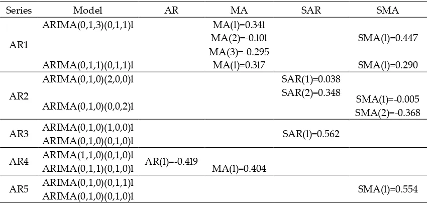
218
the additive Holt-Winters method is appropriate. Then the time series can be described in Equation
219
(2).
220
𝑌𝑡= (𝛽0+ 𝛽1𝑡) + 𝑆𝑡+ 𝜖𝑡, (2)
221
where β1 is growth rate; St is a seasonal pattern; 𝜖𝑡 is error term.
222
For such time series, the mean, the growth rate, and the seasonal variation may be changing over
223
time. A state space model for these changing components can be found in Equation (3-6).
224
225
𝑙𝑡= 𝑙𝑡−1+ 𝑏𝑡−1+ 𝛼[𝑌𝑡− (𝑙𝑡−1+ 𝑏𝑡−1+ 𝑆𝑡−𝐿)], (3)
𝑏𝑡= 𝑏𝑡−1+ 𝑏𝑡−1+ 𝛼𝛾[𝑌𝑡− (𝑙𝑡−1+ 𝑏𝑡−1+ 𝑆𝑡−𝐿)], (4)
𝑆𝑡= 𝑆𝑡−𝐿+ (1 − 𝛼)𝛿[𝑌𝑡− (𝑙𝑡−1+ 𝑏𝑡−1+ 𝑆𝑡−𝐿)], (5)
𝑌̂𝑡= 𝑙𝑡−1+ 𝑏𝑡−1+ 𝑆𝑡−𝐿, (6)
226
To begin the estimation the initial values for level, growth rate and seasonal variation should be
227
estimated. Hence, first, a least squares regression model should be generated based on available data.
228
The regression model can be expressed in Equation (7). The initial values 𝑙0, 𝑏0were also obtained
229
from the model.
230
𝑌̂𝑡= 𝑙0+ 𝑏0𝑡, (7)
231
Obtain estimated values for each time period based on the above regression model. The initial
232
seasonal factor in each of L seasons can be calculated in Equation (8-11).
233
𝑆𝐿1=
(𝑦1− 𝑦̂1) + (𝑦1+𝐿− 𝑦̂1+𝐿) + (𝑦1+2𝐿− 𝑦̂1+2𝐿) + ⋯ + (𝑦1+𝑛𝐿− 𝑦̂1+𝑛𝐿)
𝐿 , (8)
𝑆𝐿2=
(𝑦2− 𝑦̂2) + (𝑦2+𝐿− 𝑦̂2+𝐿) + (𝑦2+2𝐿− 𝑦̂2+2𝐿) + ⋯ + (𝑦2+𝑛𝐿− 𝑦̂2+𝑛𝐿)
𝐿 , (9)
𝑆𝐿3=
(𝑦3− 𝑦̂3) + (𝑦3+𝐿− 𝑦̂3+𝐿) + (𝑦3+2𝐿− 𝑦̂3+2𝐿) + ⋯ + (𝑦3+𝑛𝐿− 𝑦̂3+𝑛𝐿)
𝐿 , (10)
𝑆𝐿𝐿 =
(𝑦𝐿− 𝑦̂𝐿) + (𝑦𝐿+𝐿− 𝑦̂𝐿+𝐿) + (𝑦𝐿+2𝐿− 𝑦̂𝐿+2𝐿) + ⋯ + (𝑦𝐿+𝑛𝐿− 𝑦̂𝐿+𝑛𝐿)
𝐿 , (11)
234
Where 𝑆𝐿1, 𝑆𝐿2, 𝑆𝐿3, ⋯ , 𝑆𝐿𝐿 are seasonal factors; L is the number of seasons in a year.
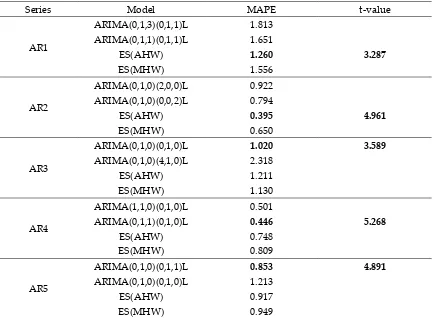
235
After finding the values for the seasonal factors, the state space models are employed to obtain
236
model parameters that minimize the sum of the squared errors. Future values of the time series are
237
predicted by the state space model in Equation (6).
238
3.3.2. Multiplicative Holt-Winters Method
If a time series has a linear trend with multiplicative seasonal variations, the multiplicative
Holt-240
Winters is appropriate to be used. The state space models for this method can be described in
241
Equations (12-15).
242
243
244
245
𝑙𝑡= 𝑙𝑡−1+ 𝑏𝑡−1+ 𝛼
[𝑌𝑡− (𝑙𝑡−1+ 𝑏𝑡−1)𝑆𝑡−𝐿]
𝑆𝑡−𝐿
, (12)
𝑏𝑡= 𝑏𝑡−1+ 𝛼𝛾
[𝑌𝑡− (𝑙𝑡−1+ 𝑏𝑡−1)𝑆𝑡−𝐿]
𝑆𝑡−𝐿
, (13)
𝑆𝑡= 𝑆𝑡−𝐿+ (1 − 𝛼)𝛿
[𝑌𝑡− (𝑙𝑡−1+ 𝑏𝑡−1)𝑆𝑡−𝐿]
𝑙𝑡
, (14)
𝑌𝑡= (𝑙𝑡−1+ 𝑏𝑡−1)𝑆𝑡−𝐿, (15)
246
And the seasonal factors can be computed in the following Equations (16-19).
247
𝑆𝐿1=
(𝑦1/𝑦̂1) + (𝑦1+𝐿/𝑦̂1+𝐿) + (𝑦1+2𝐿/𝑦̂1+2𝐿) + ⋯ + (𝑦1+𝑛𝐿/𝑦̂1+𝑛𝐿)
𝐿 , (16)
𝑆𝐿2=
(𝑦2/𝑦̂2) + (𝑦2+𝐿/𝑦̂2+𝐿) + (𝑦2+2𝐿/𝑦̂2+2𝐿) + ⋯ + (𝑦2+𝑛𝐿/𝑦̂2+𝑛𝐿)
𝐿 , (17)
𝑆𝐿3=
(𝑦3/𝑦̂3) + (𝑦3+𝐿/𝑦̂3+𝐿) + (𝑦3+2𝐿/𝑦̂3+2𝐿) + ⋯ + (𝑦3+𝑛𝐿/𝑦̂3+𝑛𝐿)
𝐿 , (18)
𝑆𝐿𝐿 =
(𝑦1/𝑦̂1) + (𝑦1+𝐿/𝑦̂1+𝐿) + (𝑦1+2𝐿/𝑦̂1+2𝐿) + ⋯ + (𝑦1+𝑛𝐿/𝑦̂1+𝑛𝐿)
𝐿 , (19)
3.4. Autoregressive Integrated Moving Average (ARIMA)
248
There are four steps to select an appropriate model for the time series data in the Box-Jenkins
249
approach [53]. The development process of an ARIMA model is shown in Figure 2. ARIMA models
250
are flexible and adaptive since they can forecast data values of a time series by a linear combination
251
of its past values, past errors (in terms of univariate analysis) and past and present values of other
252
time series (in terms of multivariate analysis). Besides, in univariate time series analysis, the
253
development processes of ARIMA models provide a comprehensive set of tools for model
254
identification, parameters estimation, diagnosis checking, and forecasting. Taking into account the
255
seasonality of the time series, a seasonal ARIMA model denoted as ARIMA (p,d,q)(P,D,Q)L is
256
introduced, where P represents seasonal autoregressive orders, D indicates seasonal differencing
257
orders, Q represents seasonal moving average orders, and L indicates the number of seasons.
258
Seasonality implies that a pattern repeats itself over a fixed time interval [54]. In this study, the
259
quarterly data present a seasonal period of four quarters. The auto-correlation function (ACF) and
260
partial auto-correlation function (PACF) were employed to determine the stationarity in the dataset.
261
The seasonal difference was used to transform the non-stationary seasonal data into stationary by
262
taking the difference between the current observation and the corresponding observation from the
263
previous year. A seasonal ARIMA model can be shown in Equation (20).
264
∅𝑝(𝐵)𝜑𝑃(𝐵𝐿)∇𝐿𝐷∇𝑑𝑦𝑡= δ + 𝜃𝑞(𝐵)𝜗𝑄(𝐵𝐿)𝑎𝑡, (20)
Where
265
𝜑𝑃(𝐵𝐿) = (1 − 𝜑1,𝐿𝐵𝐿− 𝜑2,𝐿𝐵2𝐿− ⋯ − 𝜑𝑃,𝐿𝐵𝑃𝐿),
𝛻𝐿𝐷𝛻𝑑𝑦𝑡= (1 − 𝐵𝐿)𝐷(1 − 𝐵)𝑑𝑦𝑡z,
𝜃𝑞(𝐵) = (1 − 𝜃1𝐵 − 𝜃2𝐵2− ⋯ − 𝜃𝑞𝐵𝑞),
𝜗𝑄(𝐵𝐿) = (1 − 𝜗1,𝐿𝐵𝐿− 𝜗2,𝐿𝐵2𝐿− ⋯ − 𝜗𝑄,𝐿𝐵𝑃𝐿),
266
where 𝐵 is backshift operator; L is the number of seasons in a year (L=4 for quarterly data and
267
L=12 for monthly data); δ is a constant term; 𝑎𝑡, 𝑎𝑡−1, ⋯ are random shocks; ∅1, ∅2, ⋯ , ∅𝑝are
non-268
seasonal autoregressive parameters; 𝜑1,𝐿, 𝜑2,𝐿, ⋯ , 𝜑𝑃,𝐿 are seasonal autoregressive parameters;
269
𝜃1, 𝜃2, ⋯ , 𝜃𝑞 are non-seasonal moving average parameters, 𝜗1,𝐿, 𝜗2,𝐿, ⋯ , 𝜗𝑄,𝐿 are seasonal moving
270
average parameters.
271
272
273
Figure 2. ARIMA model development process
274
3.4.1. Stationary Checking
275
Classical ARIMA models are usually used to describe stationary time series. Thus, in order to
276
identify an appropriate ARIMA model, the stationary of the times series should be determined at
277
first. If the time series is not stationary, the transformation of the time series to stationary should be
278
undertaken. A stationary time series can be described as the statistical properties (e.g. the mean and
279
the variance) of it are essentially constant over time [49]. The first differences of the non-stationary
280
time series are usually employed to transform the non-stationary time series values into stationary
281
time series values. The first differences of the time series values are shown in Equation (21).
282
283
𝑧𝑡= 𝑦𝑡− 𝑦𝑡−1, (21)
where 𝒛𝒕 indicates the first differences time series values; 𝒚𝒕 indicates non-stationary times
285
series values.
286
If a seasonal time series was analyzed, then a seasonal transformation is used to produce a
287
stationary time series. The first seasonal differencing can be described in Equation (22).
288
289
𝑧𝑡= 𝑦𝑡− 𝑦𝑡−𝐿, (22)
where L indicate the numbers of seasons in a year (L=4 for quarterly data and L=12 for monthly
290
data).
291
Moreover, the first regular differencing and seasonal differencing was usually adopted to
292
transform a seasonal non-stationary series to a stationary time series. The transformation is expressed
293
in Equation (23).
294
295
𝑧𝑡= (𝑦𝑡− 𝑦𝑡−1) − (𝑦𝑡−𝐿− 𝑦𝑡−𝐿−1) = 𝑦𝑡− 𝑦𝑡−1− 𝑦𝑡−𝐿+ 𝑦𝑡−𝐿−1, (23)
Further, the sample auto-correlation function (SAC) also can be used to determine whether the
296
time series is stationary. For example, if the SAC of a time series values either dies down quickly or
297
cuts off quickly at both seasonal lags and non-seasonal lags, then the time series can be considered as
298
stationary. If the SAC of the time series values dies down extremely slowly either at seasonal lags or
299
non-seasonal lags, it is reasonable to decide the time series is non-stationary.
300
3.4.2. Tentative Identification
301
The identification of the ARIMA models is usually dependent on the sample auto-correlation
302
function (SAC) and the sample partial auto-correlation function (SPAC) for the values of a stationary
303
time series. The behaviour of the SAC and SPAC at the seasonal level to be that at lags L, 2L, 3L, and
304
4L. The sample autocorrelation at lag k can be calculated through Equation (24).
305
306
𝑟𝑘 =
∑𝑛−𝑘𝑡=1(𝑧𝑡− 𝑧̅)(𝑧𝑡+𝑘− 𝑧̅)
∑𝑛𝑡=1(𝑧𝑡− 𝑧̅)2
, (24)
Where 𝑧𝑡 indicates the stationary time series values; 𝑧̅ is the mean of the time series.
307
The formula for the sample partial autocorrelation at lag k is presented in Equation (25).
308
309
𝑟𝑘𝑘= [
𝑟1 𝑖𝑓 𝑘 = 1
𝑟𝑘− ∑𝑘−1𝑗=1𝑟𝑘−1,𝑗𝑟𝑘−𝑗
1 − ∑𝑘−1𝑗=1𝑟𝑘−1,𝑗𝑟𝑗
𝑖𝑓 𝑘 = 2, 3, …], (25)
310
Where
311
𝑟𝑘𝑗= 𝑟𝑘−1,𝑗− 𝑟𝑘𝑘𝑟𝑘−1,𝑘−𝑗,
312
3.4.3. Parameter Estimation
313
After identifying a tentative model for a time series, the parameters of the model should be
314
estimated. The parameters are usually estimated by the least square method. The least square
315
estimation method means that the model parameters minimize the sum of the squared errors. The
316
sum of the squared errors can be computed by using Equation (26).
𝑆𝑆𝐸 = ∑(𝑦𝑡− 𝑦̂𝑡)2 𝑛
𝑡=1
, (26)
Where 𝑦𝑡 is the real value of the time series; 𝑦̂𝑡 is the value estimated by the tentative model.
319
3.4.4. Diagnostic Checking
320
The obtained models should be checked for whether the ARIMA assumptions are satisfied. As
321
a more accurate test, the Ljung-Box test is usually undertaken to examine whether the autocorrelation
322
of the residuals are statistically different from an expected white noise process. If the p-value is
323
greater than 0.05, indicating no significant autocorrelation in residuals, in turn, the model is adequate
324
[55].
325
3.4.5. Forecasting Error Measure
326
Although a model may well fit the historical data, it is not valid to determine that the model has
327
good forecasting performance. The forecasting performance of a model can only be determined by
328
the accuracy of the out-of-sample forecasts [56]. The accuracy of the forecasts was evaluated by mean
329
absolute percentage error (MAPE) between the actual and predicted values of building cost. The
330
lower the values are, the better the forecasting performance of the proposed model.
331
The most widely used criterion for forecasting models is accuracy, which has many forms,
332
including root mean square error (RMSE) [57], mean absolute error (MAE) [58], and mean absolute
333
percentage error (MAPE) [59]. This study evaluated the accuracy of the forecasts by mean absolute
334
percentage error (MAPE) between the actual and predicted values of building cost. The lower the
335
values are, the better the forecasting performance of the proposed model. Denote the real
336
observations for the time series by (𝑦𝑖) and the forecasting values for the same series by (𝑦̂𝑖). Mean
337
absolute percentage error (MAPE) can be computed in Equation (27).
338
339
𝑀𝐴𝑃𝐸 =
∑ |𝑦𝑖− 𝑦̂𝑖
𝑦𝑖 | 𝑛
𝑖=1
𝑛 × 100%,
(27)
3.5. t-Test
340
The t-test is a statistical method that is also referred to as the Student’s t-test. The t-test includes
341
one-sample t-test, two independent samples t-test, and paired sample t-test (2). Unlike some
342
statistical methods that heavily rely on sample size for their effectiveness, the t-test can be used with
343
small sample sizes (such as n <30) [60]. The t-test can be used to test the difference between one sample
344
and a set mean value (one sample t-test). The t-test can also be used to compare the difference between
345
the mean of two samples (two sample t-test). Also, it can be used to test the mean difference between
346
paired samples before and after the experiment (paired sample t-test). In this study, the paired sample
347
t-test was used. To calculate t-value, Equation (28) was used, as follows.
348
349
𝑡 = (∑ 𝐷
𝑛 𝑖=1 )/𝑁
√∑ 𝐷2− (∑ 𝐷
𝑛
𝑖=1 )2/𝑛 𝑛
𝑖=1
(𝑁 − 1)𝑁 ,
(28)
350
Where D is the difference between sample x and y and n is the sample size.
351
Then, the t-value can be calculated. Next, the t-critical value is calculated based on the sample
352
size n. If the t-value is greater than the t critical value, there is no significant difference between the
two samples. If the t-value is less than the t-critical value, there is a significant difference between the
354
two samples.
355
356
357
4. Data Analysis
358
4.1. Correlation Analysis Results
359
Correlation analysis was performed to examine whether there is a significant correlation
360
between household energy use and residential building costs, which indicated the reliability of using
361
residential building costs as an indicator of the future trend of household energy use. Based on the
362
correlation coefficient, the results of correlation analysis show a significant correlation between the
363
two variables. The significance level of the variables is validated by two-tailed significant correlation
364
values at the 0.05 level.
365
Correlation analysis was conducted using the statistical software program SPSS (Statistical
366
Packages for the Social Sciences, versions 23). Results of the analysis indicated that residential
367
building costs positively correlate with household energy use. This significant correlation supports
368
the research hypothesis. Therefore, there is a significant correlation between the energy use and
369
residential building costs. The researcher predicts the correlation between residential building costs
370
and household energy use. The results of correlation analysis are essential for understanding the
371
effectiveness of residential building costs to serve as an indicator of future trends of household energy
372
use.
373
The results of correlation analysis between household energy use variables and residential
374
building cost are shown in Table 1, which shows that all household energy use variables are
375
positively correlated with residential building costs. The highest correlation coefficient was obtained
376
from the correlation between household gas use and residential building cost of two-story house
377
(AR2), with a significant value of r = 0.994. A weakest correlation was observed between household
378
petrol use and residential building cost of retirement village (AR5), with a coefficient of r = 0.640.
379
Despite having a relative weak correlation, all the household energy use variables correlate with
380
residential building cost at a significant level.
381
Table 1. Correlation analysis results.
382
Residential Building Cost
Energies AR1 AR2 AR3 AR4 AR5
Electricity 0.974** 0.977** 0.984** 0.782** 0.833**
Gas 0.976** 0.994** 0.968** 0.966** 0.898**
Petrol 0.919** 0.916** 0.937** 0.884** 0.640**
** indicate significance at 0.05 level.
383
4.2. Exponential Models for Building Cost
384
Both additive Holt-Winters and multiplicative Holt-Winters models were applied to the five cost
385
series. Following the methods outlined in [50], the model parameters were estimated. The results of
386
the exponential smoothing models for the cost of the five categories of the residential building are
387
displayed in Table 2. The p-value of the model parameters indicate that they are effective. Moreover,
388
the model fit R-square and error measures including root mean square error (RMSE), mean absolute
389
percentage error (MAPE), and mean absolute error (MAE) were also generated. In addition, the
390
model parsimony measure Bayesian Information Criterion (BIC) was also obtained. The results are
391
shown in Table 4. They all indicate Holt-Winters models can fit the cost series fairly well because the
392
models can identify the trend and seasonal variation.
395
396
397
398
399
400
401
Table 2. Estimated parameter values with significant test for exponential smoothing models
402
Series Exponential Smoothing model Parameter Estimate SE p-value
α 0.370 0.116 0.002
ES(AHW) β 0.634 0.287 0.032**
AR1 γ 0 0.112 0.993
α 0.379 0.112 0.001**
ES(MHW) β 0.537 0.251 0.037**
γ 0.528 0.171 0.003**
α 0.899 0.150 ***
ES(AHW) β 0 0.047 1
AR2 γ 0 0.696 1
α 0.846 0.145 ***
ES(MHW) β 0.001 0.045 0.983
γ 0.028 0.298 0.925
α 0.683 0.135 ***
ES(AHW) β 0.218 0.113 0.059*
AR3 γ 0.001 0.171 0.995
α 0.578 0.128 ***
ES(MHW) β 0.269 0.128 0.042**
γ 0.020 0.091 0.830
α 0.200 0.079 0.014**
ES(AHW) β 1.000 0.467 0.037**
AR4 γ 0 0.091 1
α 0.198 0.083 0.021**
ES(MHW) β 1.000 0.503 0.052*
γ 0.040 0.062 0.524
α 0.469 0.118 ***
ES(AHW) β 0.441 0.194 0.027**
AR5 γ 0.014 0.096 0.883
α 0.361 0.096 ***
ES(MHW) β 0.511 0.225 0.028**
γ 0.479 0.151 0.003**
** indicate significance at 0.05 level, *** indicate significance at 0.01 level.
403
4.3. Seasonal ARIMA Models
404
4.3.1. Model Selection
405
[16] suggested that to properly implement the ARIMA method a time series with at least 30
406
observations is required. In this study, for each cost series, a total of 52 observations from 2001:Q1 to
407
2013:Q4 were used to obtain the proposed models. For the stationary analysis of the five cost series
408
autocorrelation function (ACF) and partial autocorrelation function (PACF) were used; results are
409
shown in Figure 3. Investigate the graphs of ACF and PACF for the five building cost series; it can be
410
observed that the ACFs decay very slowly at both non-seasonal and seasonal lags. For each cost
series, the appropriate number of differencing should be determined. Hence, it is reasonable to
412
transform to a stationary series by taking four quarter differencing of data to remove seasonality and
413
regular differencing to remove trends for the four cost series, except the cost series for the two-story
414
house in New Zealand. The cost series has only made a regular differencing to transform the data
415
into stationary. After the differencing, the results of ACFs and PACFs for the five cost series are
416
shown in Figure 4. The seasonal ARIMA models for the five cost series are shown in Table 3.
418
Figure 3. Sample ACF (left panels) and sample PA
420
421
Figure 4. ACFs (left panels) and PACFs (right panels) of the differenced data series
423
Table 3. Estimated parameter values for seasonal ARIMA models
424
Series Model AR MA SAR SMA
AR1
ARIMA(0,1,3)(0,1,1)l
ARIMA(0,1,1)(0,1,1)l
MA(l)=0.34l MA(2)=-0.l0l MA(3)=-0.295
MA(l)=0.3l7
SMA(l)=0.447
SMA(l)=0.290
AR2
ARIMA(0,1,0)(2,0,0)l
ARIMA(0,1,0)(0,0,2)l
SAR(1)=0.038 SAR(2)=0.348
SMA(l)=-0.005 SMA(2)=-0.368
AR3 ARIMA(0,1,0)(1,0,0)l
ARIMA(0,1,0)(0,1,0)l SAR(l)=0.562
AR4 ARIMA(1,1,0)(0,1,0)l
ARIMA(0,1,1)(0,1,0)l AR(l)=-0.4l9 MA(l)=0.404
AR5 ARIMA(0,1,0)(0,1,1)l
ARIMA(0,1,0)(0,1,0)l SMA(l)=0.554
425
4.3.2. Proposed Seasonal ARIMA Models
426
Based on the approach provided by [53], the model parameters, model fit, and error measures
427
were estimated for the five cost series. In order to select proper seasonal ARIMA models, different
428
models with various combinations of regular orders (p and q) and seasonal orders (P and Q) were
429
evaluated. The model parameters of the five cost series are presented in Table 3. Furthermore, the
430
model fit and error measures of the ARIMA models are provided in Table 4. As seen from Table 4,
431
ARIMA models fit the cost data fairly well.
432
4.3.3. Model Validation
433
The Ljung-Box Q test was employed to examine the autocorrelation of model residuals. If the
p-434
value is greater than the value of 0.05, the null hypothesis that the data are not correlated should be
435
accepted [16]. To examine the normality of the residuals the analysis applied the Shapiro-Wilk test.
436
If the p-value of the test is greater than the value of 0.05, it indicates that there is no evidence to reject
437
the null hypothesis that the data follow a normal distribution [61]. As seen from Table 4, the residuals
438
of all the models pass the tests, indicating the proposed models are adequate. According to the
439
estimation results, the model fit measures and error measures are acceptable. This suggests that the
440
proposed models fit the data fairly well.
456
457
Table 4. Model fit statistics and residual statistics
458
Series Model
R-Square RMSE MAPE MAE BIC
Ljung-Box
Shapiro-Wilk
AR1
ARIMA(0,1,3)(0,1,1)4 0.959 37.234 1.716 25.866 7.644 0.873 0.461 ARIMA(0,1,1)(0,1,1)4 0.953 38.665 1.856 27.895 7.556 0.519 0.158 ES(AHW) 0.976 33.205 1.655 24.52 7.233 0.238 0.203 ES(MHW) 0.974 34.311 1.581 23.722 7.299 0.805 0.102
AR2
ARIMA(0,1,0)(2,0,0)4 0.942 63.899 2.221 38.057 8.546 0.877 0.184 ARIMA(0,1,0)(0,0,2)4 0.942 63.865 2.256 38.766 8.545 0.898 0.136 ES(AHW) 0.947 62.506 2.066 35.292 8.498 0.891 0.153 ES(MHW) 0.943 64.989 2.159 37.134 8.576 0.904 0.133
AR3
ARIMA(0,1,0)(0,1,0)4 0.944 54.277 1.913 35.836 8.07 0.855 0.153 ARIMA(0,1,0)(4,1,0)4 0.95 53.423 1.823 33.945 8.366 0.956 0.122 ES(AHW) 0.964 52.405 1.953 36.27 8.146 0.13 0.103 ES(MHW) 0.959 55.473 2.054 38.568 8.26 0.106 0.173
AR4
ARIMA(1,1,0)(0,1,0)4 0.981 51.468 1.53 37.383 8.046 0.657 0.391 ARIMA(0,1,1)(0,1,0)4 0.981 51.889 1.505 36.868 8.062 0.628 0.24
ES(AHW) 0.989 45.577 1.32 31.825 7.867 0.593 0.127 ES(MHW) 0.988 47.836 1.385 34.24 7.964 0.333 0.104
AR5
ARIMA(0,1,0)(0,1,1)4 0.986 40.162 1.325 27.306 7.55 0.489 0.127 ARIMA(0,1,0)(0,1,0)4 0.983 43.299 1.52 31.335 7.618 0.141 0.103 ES(AHW) 0.991 36.083 1.312 27.824 7.4 0.477 0.393 ES(MHW) 0.989 39.374 1.356 28.715 7.574 0.415 0.647
459
5. Model Selection
460
5.1. Comparisons of the Models
461
Although a model can fit the data fairly well, it does not indicate that the model can produce
462
better forecasts [62]. The forecasting accuracy of a model is affected by many factors, such as the
463
number of observations in the time series, the number of forecast time origins examined, and the
464
number of forecast lead times regarded [63]. In general, exponential smoothing models outperform
465
ARIMA models in predicting in sample period. Despite superior performance over the in-sample
466
period, the good performance of the exponential smoothing models does not translate into
out-of-467
sample forecasts. However, seasonal ARIMA models are able to produce consistent forecasts based
468
on error measures.
469
The forecasting performance of the univariate methods was evaluated by MAPE statistics. The
470
results for residential building cost of one-story house (AR1) presented in Table 5 suggest that the
471
exponential smoothing models generate better results in comparison to seasonal ARIMA models. In
472
particular, the additive Holt-Winters model produces better forecasts based on MAPE measurement.
473
When analyzing the results for cost of two-story house (AR2), the additive Holt-Winters model
474
outperforms other models based on MAPE measurement. The results regarding cost of townhouse
475
(AR3), the ARIMA model has the best forecasting performance among the proposed four models. For
476
results for cost of apartment (AR4) suggest that ARIMA (0,1,1) (0,1,0)4 is the best forecasting model.
477
For results considering cost of retirement village (AR5), ARIMA (0,1,0) (0,1,1)4 produced the best
478
forecasts among the proposed models. Therefore, these results suggest that the ARIMA approach is
better than the exponential smoothing method for building cost of the town house (AR3), apartment
480
(AR4) and retirement village (AR5) in New Zealand. Although the seasonal ARIMA models did not
481
outperform exponential smooth models in the model training process, their error measures are
482
slightly larger than that of exponential models. The results show that seasonal ARIMA models
483
perform better for predicting building cost for town house, apartments and retirement village in New
484
Zealand, while exponential smooth models are superior in cost forecasting for both the one-story
485
house and the two-story house in New Zealand. This outcome may be due to the relative stability of
486
the cost series for the one-story house and the two-story house.
487
From the above results, it can be seen that both the exponential smoothing method and the
488
ARIMA approach can produce good forecasts for residential building cost in New Zealand. Which
489
method is better, depends on the characteristics of the data. For example, the ARIMA approach can
490
produce better forecasts for building costs of town house, apartment and retirement village, which
491
indicates that these costs have a random walk characteristic.
492
The MAPE of the proposed models for all the five cost series are presented in Table 5. Bold type
493
is utilized in these tables to identify the lowest values of MAPE for each proposed model. As the
494
results show, no single forecasting method is better for all data series. This confirms the generally
495
acceptable idea that no individual forecasting approach can describe all the situations [64].
496
Table 5. Forecast values for building cost of one-story house in New Zealand
497
Series Model MAPE t-value
AR1
ARIMA(0,1,3)(0,1,1)L 1.813
ARIMA(0,1,1)(0,1,1)L 1.651
ES(AHW) 1.260 3.287
ES(MHW) 1.556
AR2
ARIMA(0,1,0)(2,0,0)L 0.922
ARIMA(0,1,0)(0,0,2)L 0.794
ES(AHW) 0.395 4.961
ES(MHW) 0.650
AR3
ARIMA(0,1,0)(0,1,0)L 1.020 3.589
ARIMA(0,1,0)(4,1,0)L 2.318
ES(AHW) 1.211
ES(MHW) 1.130
AR4
ARIMA(1,1,0)(0,1,0)L 0.501
ARIMA(0,1,1)(0,1,0)L 0.446 5.268
ES(AHW) 0.748
ES(MHW) 0.809
AR5
ARIMA(0,1,0)(0,1,1)L 0.853 4.891
ARIMA(0,1,0)(0,1,0)L 1.213
ES(AHW) 0.917
ES(MHW) 0.949
498
5.2. t-Test results
499
In this study, the paired sample t-test was used to compare the mean difference between the
500
estimated residential building cost with the real residential building cost. The t-test was performed
501
using SPSS. The t-value was greater than the t-critical value (t-critical=1.666, n = 72), which means
502
there is no significant difference between the real residential building costs and the estimated
503
residential building costs. The t-value for the best-fit models are shown in Table 5.
505
506
507
6. Results Discussion
508
Correlation analysis was performed to test the correlation between residential energy use and
509
residential building costs. These results validate that a correlation still exists between household
510
energy use (electricity, gas, petrol) and estimated residential building cost at a significant level.
511
Exponential smoothing (ES) approach and ARIMA technique are both effective time series
512
forecasting methods as they both can fairly well describe trend movement in the time series, but they
513
have both strengths and weaknesses. For example, the ARIMA approach is more readily expanded
514
to model interventions, outliers, variations and variance changes in time series; but it is a relatively
515
sophisticated technique. Due to different data patterns and limited sample size, it is unjust to attempt
516
to determine whether one time series forecasting method is better than the other. Therefore, either
517
the exponential smoothing method or the ARIMA approach should be given a chance to demonstrate
518
its maximum potential in any empirical case study.
519
While ES method is based on describing the trend and seasonality in the time series, ARIMA
520
approach is focused on a description of the autocorrelation in the data. There is an idea that ARIMA
521
approach is more advanced than ES method since the former has fewer parameters to be estimated.
522
Although ARIMA models are more general, ES models can provide framework that is sufficient to
523
capture the dynamics in the data series. ARIMA models are excellent for short-term forecasting.
524
When they are used for long-term forecasting, the models need to be remodeled based on updated
525
data incorporated into the model training process. ES method can be very competitive by
526
automatically incorporating updated information into the model, and then producing better forecasts
527
for long-term forecasting. An advantage of ARIMA technique is that only several parameters need to
528
be estimated for generating good forecasting results. However, extreme values in the dataset are
529
difficult to be estimated by ARIMA models due to the univariate nature of the model and the lack of
530
a specific ability to simulate unexpected events.
531
In fact, for all the five cost series of residential building in New Zealand to which the statistical
532
approaches were applied, the exponential smoothing models showed an excellent performance at the
533
model training phase. However, seasonal ARIMA models produced more accurate forecasts for cost
534
series of the town house, apartment and retirement village in the forecasting process. In the case of
535
the cost for town house, apartment, and retirement village in New Zealand, the cost data must be
536
examined in greater detail to identify previous short-term variations. Any distinct changes in the cost
537
series may result in ARIMA models being wholly unsuitable.
538
7. Conclusions
539
Several methods have been used to predict future household energy use, but most of them are
540
based on building factors such as thermal envelope or HVAC systems. However, in this study,
541
residential building cost was used as an indicator of future trends of household energy use.
542
Correlation analysis showed a significant positive correlation between household energy use and
543
residential building cost. This result not only provides a clear guide for the future trend of household
544
energy use, but also forms the relationship between the house building costs at the construction stage
545
and the energy used at the operational stage. It is not necessary to evaluate every component of the
546
building; future trends of energy use can be obtained from the residential building cost. In addition,
547
results of correlation analysis will help developers or investors to make informed decisions by
548
connecting current investment (construction cost) and future expenses (energy used). Accurate
549
prediction of residential building cost provides a clear indication of the future trend of household
550
energy use.
551
In this study, quarterly building costs data (over an 18-year range 2001:Q1-2018:Q4) for five
552
categories of residential building (one-story house, two-story house, town house, apartment, and
retirement village) in New Zealand, were analyzed. It was found that time series data of residential
554
building costs are non-stationary and autocorrelated and do not display a very strong seasonal
555
pattern. Based on the identified characteristics, two time series forecasting techniques, exponential
556
smoothing method and ARIMA approach, were adopted to take into account variations of residential
557
building costs in predicting their future trends. It was concluded that both methods can produce
558
proper forecasts. The analysis of model residuals explored that the underlying modelling
559
assumptions hold true.
560
The primary contributions of this study to the existing body of knowledge are twofold: (1)
561
explore the relationship between residential energy use and residential building costs; and (2)
562
develop univariate forecasting models to predict the future trend of residential building cost with
563
reasonable accuracy. The findings of this study can help industry professionals prepare energy use
564
plan, help in decision making, and provide a new clue for energy management. Although this study
565
used the QV's residential building cost index and energy variables of Statistics New Zealand, the
566
proposed methods can be used for similar data sets in other cities as well as globally. Although these
567
forecasting techniques are to predict future values of building cost, they can be further applied to
568
other modelling purposes.
569
Abbreviations
570
571
ACF Auto-Correlation Function
AR Autoregressive
AR1 One-story House
AR2 Two-story House
AR3 Townhouse
AR4 Apartment
AR5 Retirement Village
ARIMA Autoregressive Integrated Moving Average BIC Bayesian Information Criterion
ES Exponential Smoothing Method
HVAC Heating, Ventilation and Air Conditioning
HW Holt-Winter Method
MA Moving Average
MAE Mean Absolute Error
MAPE Mean Absolute Percentage Error MHW Multiplicative Holt-Winter Method PACF Partial Auto-Correlation Function PPP Public-Private Partnership RMSE Root Mean Square Error
SAC Sample Auto-Correlation Function SAR Seasonal Autoregressive
SE Standard Error
SMA Seasonal Moving Average
SPAC Sample Partial Auto-Correlation Function
572
573
575
576
577
Author Contributions: Conceptualization, L.Z. and J.M.; methodology, L.Z.; software, Z.L.; validation, L.Z.,
578
Z.L.; writing—original draft preparation, L.Z.; writing—review and editing, J.M.; supervision, J.M.; project
579
administration, J.M.; funding acquisition, L.Z
580
Funding: This research was funded by China Scholarship Council, grant number 201206130069, Massey
581
University, grant number 09166424, and Beijing University of Technology, the grant number is 004000514119067.
582
The APC was funded by the three grants.
583
Acknowledgments: The authors would like to thank the China Scholarship Council (CSC) for its support
584
through the research project and also the Massey University. The authors would like to thank Reserve Bank of
585
New Zealand and Ministry of Business, Innovation, and Employment for providing data to conduct this
586
research. In addition, I would like to thank all practitioners who contributed to this project.
587
Conflicts of Interest: The authors declare no conflict of interest.
588
589
References
590
591
1. Reinisch, C.; Kofler, M.; Iglesias, F.; Kastner, W., Thinkhome energy efficiency in future smart homes.
592
EURASIP Journal on Embedded Systems 2011, 104617.
593
2. Lee, Y. M.; An, L.; Liu, F.; Horesh, R.; Chae, Y. T.; Zhang, R., Applying science and mathematics to
594
big data for smarter buildings. Annals of the New York Academy of Sciences 2013, 1295 (1), 18-25.
595
3. Li, D. H. W.; Yang, L.; Lam, J. C., Impact of climate changes on energy use in the built environment in
596
different climate zones-A review. Energy 2012, 42 (1), 103-112.
597
4. Murphy, K. D.; McCartney, J. S., Seasonal response of energy foundations during building operation.
598
Geotechnical and Geological Engineering 2014, 33 (2), 343-356.
599
5. Buildings Department Comprehensive environmental performance assessment scheme for buildings: CEPAS
600
application guidelines; HKSAR Government: HK, 2006.
601
6. Muringathuparambila, R. J.; Musangoa, J. K.; Brentb, A. C.; Curriea, P., Developing building typologies
602
to examine energy efficiency in representative low cost buildings in Cape Town townships. Sustainable Cities and
603
Society 2017, 33, 1-17.
604
7. Copiello, S., Achieving affordable housing through energy efficiency strategy. Energy Policy 2015, 85,
288-605
298.
606
8. Konstantinidou, C. A.; Lang, W.; Papadopoulos, A. M., Multiobjective optimization of a building
607
envelope with the use of phase change materials (PCMs) in Mediterranean climates. International Journal of Energy
608
Research 1, 1-18.
609
9. Abdallah, M.; El-Rayes, K.; Liu, L., Economic and GHG emission analysis of implementing sustainable
610
measures in existing public buildings. Journal of Performance of Constructed Facilities 2016, 30 (6), 1-14.
611
10. Groissböck, M.; Heydari, S.; Mera, A.; Perea, E.; Siddiqui, A. S.; Stadler, M., Optimizing building
612
energy operations via dynamic zonal temperature settings. Journal of Energy Engineering 2014, 140 (1), 1-10.
613
11. Byun, J.; Shin, T., Design and Implementation of an energy-saving lighting control system considering user
614
satisfaction. IEEE Transactions on Consumer Electronics 2018, 64 (1), 61-68.