Climate Policy Implications of Nonlinear Decline of Arctic Land Permafrost and Sea Ice
Dmitry Yumashev1,6*, Chris Hope2, Kevin Schaefer3, Kathrin Riemann-Campe4, Fernando Iglesias-Suarez5, Elchin Jafarov3, Gail Whiteman1, Paul Young5
1 Pentland Centre for Sustainability in Business, Lancaster University, Lancaster, UK,
[email protected]; [email protected]
2 Judge Business School, University of Cambridge, Cambridge, UK
3 National Snow and Ice Data Centre, Cooperative Institute for Research in Environmental Sciences,
University of Colorado, Boulder, Colorado, USA
[email protected]; [email protected]
4 Alfred Wegener Institut, Helmholtz Zentrum für Polar- und Meeresforschung,Bremerhaven,
Germany
5 Lancaster Environment Centre, Lancaster University, UK
[email protected]; [email protected]
6 Rotterdam Management School, Erasmus University Rotterdam, Rotterdam, Netherlands
*corresponding author
Abstract
Arctic feedbacks will accelerate climate change and could jeopardise mitigation efforts. The permafrost carbon feedback releases carbon to the atmosphere from thawing permafrost and the sea ice albedo feedback increases solar absorption in the Arctic Ocean. A constant positive albedo feedback and zero permafrost feedback have been used in nearly all climate policy studies to date, while observations and models show that the permafrost feedback is significant and that both feedbacks are nonlinear. Using novel dynamic emulators in the integrated assessment model PAGE-ICE, we investigate nonlinear interactions of the two feedbacks with the climate and economy under a range of climate scenarios consistent with the Paris Agreement. The permafrost feedback interacts with the land and ocean carbon uptake processes, and the albedo feedback evolves through a sequence of nonlinear transitions associated with the loss of Arctic sea ice in different months of the year. The US’s withdrawal from the current national pledges could increase the total discounted economic impact of the two Arctic feedbacks until 2300 by $25 trillion, reaching nearly $120 trillion, while meeting the 1.5 °C and 2 °C targets will reduce the impact by an order of magnitude.
Keywords: climate change; cryosphere; Arctic; permafrost; sea ice; tipping elements; climate impacts; climate policy; Paris agreement
The Arctic region is warming twice as fast as the global average,1 manifested by a decrease in sea ice and glaciers and permafrost degradation relative to their benchmark average states for the period between 1979 and 2005.2,3,4,5 These changes can accelerate the warming further through a variety of climatic feedbacks. The permafrost carbon feedback (PCF)6,7 releases carbon into the atmosphere
from thawing permafrost,i and the sea ice-albedo feedback (SIAF)8,9 increases solar absorption in the Arctic Ocean. Despite significant advances documented by the 5th IPCC Assessment Report, projections of future climate using state-of-the-art Earth system models (ESMs) from the CMIP5 project do not include PCF, 10,11 although several models will incorporate the PCF in the 6th assessment report.ii Consequently, most climate policy assessments based on results from the ESMs underestimate the extent of warming in response to anthropogenic emissions. The SIAF, on the other hand, is present in climate projections by the ESMs through the coupling of sea ice models to atmosphere and ocean models.10 However, existing estimates of the total economic impact of climate change under different policy assumptions using integrated assessment models (IAMs) assume that radiative forcing from SIAF increases linearly with global mean temperature, which is inconsistent with the predictions of the ESMs.iii
The Paris Agreement of December 2015 sets out ambitious targets to “limit global mean temperature rise well below 2°C and, if possible, below 1.5°C above pre-industrial levels,” which are more challenging than the current set of intended nationally determined contributions (INDCs).12 Achieving these targets represents a significant challenge to the international community.13,14 The framework set out by the Paris Agreement and its implementation continue to face political hurdles, epitomised by the recent decision of the United States Federal Government to withdraw from it.15
PCF and SIAF represent three of the thirteen main tipping elements the Earth’s climate system identified in a recent survey by Schellnhuber et al.16 Tipping elements are physical processes acting as positive nonlinear climate and biosphere feedbacks that could accelerate global warming significantly and cause substantial impacts on ecosystems, economies and societies throughout the world if certain thresholds are passed. They are likely to impact the world’s ability to achieve the specific climate targets outlined in the Paris Agreement, and highlight the importance of the more ambitious 1.5°C and 2°C targets.17 We already see notable changes not only in the tipping elements like Arctic summer sea ice, which are expected to be triggered under moderate temperature increases, but also in the more resilient Arctic winter sea ice.18 Permafrost is also in decline,5 although its nature as a tipping element is being debated in the scientific community.iv
Here we explore the climatic and economic impacts of the PCF and SIAF using model emulators, which are simple statistical representations of output from much more complicated physical models. The climatic impacts focus on changes in the global mean surface temperature (GMST) and the economic impacts focus on the net present value (NPV) of the total cost associated with future climate change. We consider a wide range of scenarios: the full Paris Agreement, the US’s withdrawal from the INDCs, the current “business as usual” (BaU) projections (no INDCs), and a pathway characterised by a very high use of fossil fuels. To perform the analysis, we use PAGE-ICE, a new development of the PAGE09
i Emissions from thawing sub-sea permafrost on Arctic shelf are poorly understood in comparison with land permafrost emissions, and therefore sub-sea permafrost is excluded from the analysis.
ii Private correspondence.
IAM19,20 that includes an internal nonlinear dynamic representation of PCF and SIAF, along with a number of updates to the science and economics in line with the latest literature.v
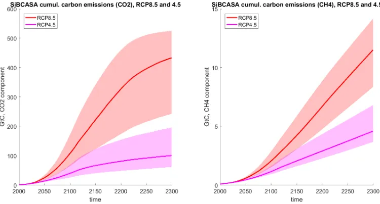
We base the PCF emulator on output from the Simple Biosphere/Carnegie-Ames-Stanford Approach (SiBCASA) terrestrial biosphere model6 driven by CMIP5 RCP8.5 and RCP4.5 simulations out to 2300 (Figure 1). The CMIP5 models used are: CNRM-CM5, GISS-E2-H, HadGEM2-ES, IPSL-CM5A-LR and MPI-ESM-LR. The dynamic PCF emulator uses a statistical fitvi to SiBCASA output for the land permafrost emissions of CO2 and methane, capturing nonlinear effects seen in the SiBCASA results.v The PAGE-ICE model adds the permafrost fluxes from the emulator to the anthropogenic global CO2 and methane emissions in each analysis year.
Figure 1. Cumulative carbon emissions from thawing land permafrost for the CO2 (left) and methane (right) components
under the RCP8.5 (red) and RCP4.5 (magenta) scenarios out to 2300. The data were generated by the SiBCASA model forced by multiple CMIP5 Earth system models (see the main text for the list). Thick lines: multi-model means; shaded areas: multi-model spread between the lowest and the highest values. Units: GtC. Note the difference in the Y-axis scale between the plots.
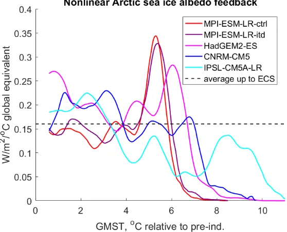
We base the SIAF emulator on monthly mean sea ice extent and GMST projections from multiple ESMs run until 2300 under the RCP8.5 scenario (Figure 2). The ESMs used are: CNRM-CM5, HadGEM2-ES and IPSL-CM5A-LR from the CMIP5 project, plus the latest available version of the MPI-ESM-LR model (1.2.00p4), which we denote as MPI-ESM-LR-ctrl, and the newly developed MPI-ESM-LR-itd modification with a novel sub-grid representation of the sea ice thickness distribution.21 The dynamic SIAF emulator accounts for nonlinear regimes in SIAF associated with the varying pace of the loss of Arctic sea ice for different seasons.22,23 It also recognises that a constant value of SIAF is implicitly included in the 2xCO2 equilibrium climate sensitivity parameter (ECS), which is central to modelling the greenhouse effect in IAMs like PAGE.vii The correction to SIAF provided by the emulator alters the governing equation for the GMST change in PAGE-ICE by adding extra terms to the total anthropogenic radiative forcing (RF) in each analysis year.
v See the Methods section and Supplementary Materials. vi See the Methods section.
This paper represents a major advance in probabilistic modelling of the nonlinear PCF and SIAF dynamically in an IAM consistent with results from state-of-the-art process-based models. We account for multiple nonlinear transitions in the intensity of the two feedbacks that have not been explored in the literature.24,25,26,27,viii This is also the first study to perform fully-coupled runs of both feedbacks combined, where PCF emissions influence the SIAF and vice versa, and is the first one to quantify the effect of CO2 land and ocean uptake on the PCF strength. The nonlinear interactions between PCF and SIAF are particularly important when analysing their climatic and economic implications across a wide spectrum of climate scenarios ranging from the ambitious 1.5°C target to the much greater warming under the RCP8.5 scenario.28 The uncertainties in PCF and SIAF are calibrated based on the expert models and are reproduced in PAGE-ICE by Monte-Carlo simulations.
Figure 2. Arctic SIAF as a function of the GMST rise relative to pre-industrial conditions, inferred from monthly mean sea ice extent and GMST projections by multiple Earth system models under the RCP8.5 scenario out to 2300. The dashed line shows the average of SIAF up to 2xCO2 equilibrium climate sensitivity (ECS) warming level (2.8°C according to CMIP5
results).
Climate scenarios and model setup in PAGE-ICE
The scenarios consistent with the Paris Agreement and current climate change projections are defined by pairing representative concentration pathways (RCPs) and shared socio-economic pathways (SSPs) according to the feasible ranges of emissions for each of the five main SSPs:29
Low emissions:
• 1.5°C target Paris: RCP2.6e & SSP1 • 2°C target Paris: RCP2.6 & SSP1
Medium emissions:
• INDCs: RCP4.5 & SSP2
• INDCs no-US: RCP4.5+ & SSP2+
High emissions:
• Current BaU projections: RCP4.5++ & SSP2++ • High fossil fuels use: RCP8.5 & SSP5
We define the 1.5°C and 2°C scenarios as having a 50% chance of keeping the GMST rise in 2100 below the 1.5°C and 2°C targets, based on PAGE-ICE simulations. These scenarios overshoot their respective GMST targets during the second half of the 21st century, and imply negative emissions thereafter. The modified RCP2.6e emissions pathway assumes extra abatement relative to RCP2.6 to achieve the 1.5°C target by 2100. The new RCP4.5+ & SSP2+ and RCP4.5++ & SSP2++ pairs assume progressive shifts from the RCP4.5 & SSP2 trajectory representing a medium use of fossil fuels towards the extensive consumption of fossil fuels as in the RCP8.5 & SSP5 scenario pair.
All the RCP scenarios in PAGE-ICE are emissions-driven,30 unlike the concentration-driven RCP scenarios that were used in most CMIP5 experiments.10 We simulated each RCP-SSP pair out to 2300 assuming constant levels of annual emissions, constant GDP growth rates and zero population growth rates beyond 2100. We used 100,000 Monte-Carlo simulations in PAGE-ICE to perform sensitivity experiments for the climatic and economic effects of PCF and SIAF. Our main results report the difference between the PAGE-ICE outputs for PCF and SIAF and their respective legacy values, defined as the values of PCF and SIAF that have been used in climate policy studies to date. For PCF, the legacy value is “zero emissions from permafrost” since PCF is not included in most climate projections using ESMs.11 For SIAF, the legacy value is “constant SIAF of 0.165 W/m2/°C”, which corresponds to 2xCO2 equilibrium climate sensitivity parameter (ECS) calibrated according to CMIP5 results. Further details are provided in the Methods section and Supplementary Materials.
Results
GMST changes due to PCF and SIAF
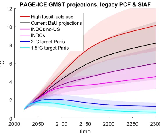
Figure 3. Monte-Carlo mean GMST projections relative to pre-industrial levels (thick lines) and the relevant uncertainty ranges (± 1 SD, shaded areas) obtained from 100,000 runs of PAGE-ICE for each of the six climate scenarios, assuming the following legacy values of PCF and SIAF: zero permafrost emissions and constant SIAF of 0.165 W/m2/°C.
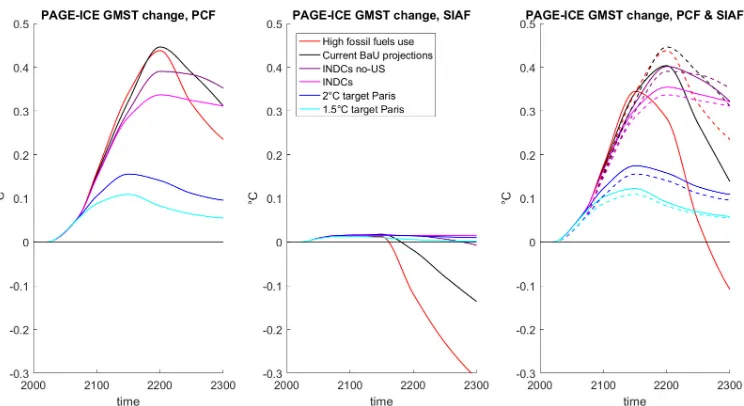
The Monte-Carlo means of the absolute changes in GMST until 2300 due to the nonlinear PCF, SIAF and PCF & SIAF combined, measured relative to their respective legacy values, are shown in Figure 4 for the six climate scenarios. The GMST changes from PCF and SIAF are smaller than the underlying uncertainty in the baseline climate projections in PAGE-ICE (Figure 3; note the different vertical scale). However, the mean values plotted in Figure 4 represent statistically significantix shifts in the state of the climate system due to the two feedbacks. For PCF, the four higher emissions scenarios lead to bigger GMST increases in 2100 compared to the two lower scenarios (~0.15°C vs. ~0.1°C).
Rather than being a tipping element, PCF responds gradually to changing climatic conditions. Its strength peaks and then declines in all scenarios (Figure 4, left), although the GMST change due to PCF is always positive because it always adds CO2 and methane to the atmosphere. There are several reasons behind this decline, depending upon the scenario. First, the marginal effect of CO2 emissions from PCF on the RF and GMST drops as atmospheric CO2 concentrations increase.19 Thus, for higher emissions scenarios the impact of adding more CO2 due to PCF decreases. Second, for the high emissions scenarios the permafrost carbon stock becomes exhausted. This leads to a rapid drop in the annual CO2 flux from permafrost beyond 2150, resulting in carbon removal from the atmosphere through CO2 ocean uptake.x The 1.5°C and 2.0°C target scenarios are different from the rest since they imply a decrease in the GMST after 2050 (Figure 3), leading to a growth of the permafrost area and refreezing of some of the thawed carbon. This reduces the amount of thawed carbon, causing a decrease in the PCF strength. These findings are in contrast to recent results based on coupled runs of the JULES and ORCHIDEE-MICT ecosystems models with the IMOGEN climate emulator, which showed a monotonous increase in the GMST effect of PCF under all scenarios.31
Figure 4. Absolute changes in GMST until 2300 due to PCF (left), SIAF (centre) and combined PCF & SIAF (right, solid lines) under the six climate scenarios. For reference, the dashed lines on the right-hand-side plot replicate the effect of PCF. 100,000 Monte-Carlo runs of PAGE-ICE. The reductions in the GMST effect of PCF and SIAF observed during the 23rd century
are explained in the text.
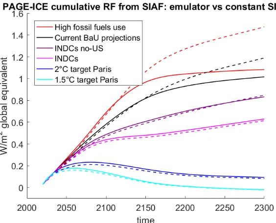
SIAF, on the other hand, evolves through a sequence of nonlinear transitions associated with the loss of Arctic sea ice in different months of the year,xi and not just in the end of the summer and winter, as stipulated by the existing theory of the tipping elements in the Earth’s climate system.16 The SIAF effect shown here (Figure 4, centre) represents the difference between the legacy constant SIAF currently assumed in IAMs and the non-linear SIAF we use. This difference is evident by comparing the cumulative RF associated with the two representations of the SIAF (Figure 5). Initially, the constant SIAF underestimates the GMST increase compared to the non-linear SIAF for all scenarios, which is due to the increased solar absorption in the Arctic ocean driven by the loss of the summer sea ice beyond 2050.xii This effect is similar for all scenarios and is an order of magnitude less than that of PCF. Summer sea ice subsequently recovers only under the 1.5°C target scenario, leading to a drop in the SIAF strength after 2150 (Figure 4, centre). For the 2°C target and INDCs scenarios, the warming effect of the non-linear SIAF relative to the constant SIAF does not change significantly after 2050. On the contrary, for the Current BaU and High fossil fuels use scenarios, the constant SIAF greatly overestimates the GMST increases compared to the non-linear SIAF beyond 2150, which is due to the loss of the winter sea ice.xii A similar but smaller effect occurs for the INDCs no-US scenario after 2250. For the High fossil fuels use scenario, the difference between the constant and non-linear SIAF becomes as large as the PCF, resulting in a negative change in GMST after 2250.
Adding the non-linear SIAF impacts to the PCF impacts on GMST tends to amplify the warming in all scenarios at all times except those with the highest atmospheric CO2 concentrations (Figure 4, right).
Figure 5. Cumulative global equivalent RF from nonlinear SIAF (solid lines) and cumulative RF corresponding to constant average SIAF of 0.165 W/m2/°C for the period between pre-industrial conditions and the 2xCO
2 ECS warming level (dashed
lines), plotted under the six climate scenarios. Mean values of 100,000 Monte-Carlo runs of PAGE-ICE.
The influence of PCF and SIAF on total economic effect of climate change
The Monte-Carlo mean NPV of the total economic effect of climate change, denoted as , consists of mitigation costs, adaptation costs and economic impacts aggregated and discounted until 2300. The default PAGE-ICE setting estimates the economic effect based on PAGE0932,33,34,35 with updates to climate impacts IPCC AR5,10 and further updates to the sea level rise driver, discontinuity impacts and mitigation costs.xiii We also consider alternative estimates for the economic impacts based on recent macro-econometric analysis of historic temperature shocks on economic growth in multiple countries by Burke et al, the most comprehensive of its kind to date.36,xiv
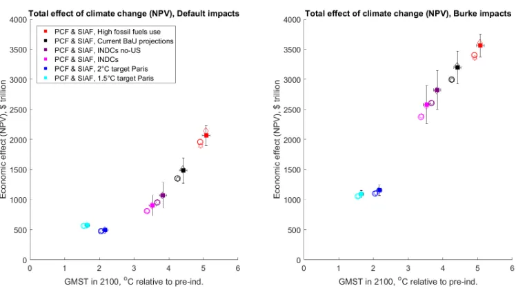
The values of for the legacy Arctic feedbacks, PCF, SIAF and PCF & SIAF combined are plotted in Figure 6 against the corresponding mean increases in GMST in 2100. They vary greatly between the six climate scenario pairs considered. The 1.5°C scenario gives a larger than the 2°C scenario under the default impacts setting, but the 1.5°C world becomes more economically attractive than the 2°C world if the Burke impacts are used. The effect of the Arctic feedbacks is relatively small under the two low emission scenarios regardless of the economic impacts evaluation used. The four higher emissions scenarios lead to progressively larger because of steep increases in the climate impacts with the temperature, and the effect of PCF and SIAF becomes stronger. The gap between the climate costs for the 1.5°C and 2°C target scenarios and for the four higher emissions scenarios is more pronounced for the Burke impacts, and so are the additional climate costs due to PCF and SIAF.
Figure 6. Monte-Carlo means of the GMST rise in 2100 and NPV of the total economic effect of climate change (until 2300) under the six climate scenarios for the default PAGE-ICE impacts setting (left) and Burke impacts (right). The effect is plotted for the legacy values of PCF and SIAF (circles), nonlinear PCF (diamonds), nonlinear SIAF relative to the constant legacy SIAF (hexagons), and for the nonlinear PCF & SIAF combined (squares). Standard deviations of the sensitivity experiments are shown for the case with both feedbacks combined. 100,000 Monte-Carlo runs of PAGE-ICE.
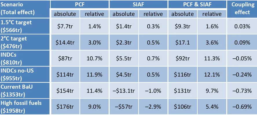
The absolute and relative changes in due to PCF and SIAF – individually and combined – with respect to the legacy values, are given in Table 1 for the default PAGE-ICE impacts setting, which is used for the remainder of the paper.xv The mean effect of PCF is always that of economic losses, which are considerably larger for the medium and high emissions scenarios compared to the 1.5°C and 2°C scenarios. The mean effect of the non-linear SIAF measured relative to the legacy SIAF value amounts to losses under the low and medium emissions scenarios. Initially 5 times weaker than PCF under the 1.5°C scenario, the losses from SIAF almost double for the 2°C scenario and then double again for the INDCs scenarios. However, at that point they are around 20 times smaller compared to PCF. Furthermore, the SIAF effect becomes negative relative to the legacy SIAF value for the Current BaU and High fossil fuels use scenarios due to the decline of the winter sea ice, which offsets some of the losses from PCF.
The case when PCF and SIAF are combined is the most realistic. The resulting nonlinear interactions of the peaks and troughs in SIAF with the varying pace of the warming and exhaustion of permafrost carbon stocks in PCF,xvi lead to additional changes in compared with the sum of each of the two effects individually. The relative magnitude of this effect under all the scenarios is given in Table 1 for the default PAGE-ICE impacts setting. Under the Current BaU scenario, the interactions between PCF and SIAF are responsible for a $10 trillion decrease in . This offsets around 7% of the effect associated with PCF alone, showing how important it is to have a correct representation of the nonlinear climate feedbacks such as PCF and SIAF in IAMs if one wants to use them to make recommendations on climate policy.
xv The estimates for the effects of PCF and SIAF based on the Burke impacts setting of PAGE-ICE are provided in Supplementary Materials.
Across all the scenarios, the combined economic losses from PCF and SIAF reach the highest value of $131 trillion under Current BaU. The US’s withdrawal from the INDCs could increase the losses by almost $25 trillion, reaching $116 trillion.
Table 1. Absolute and relative changes in due to PCF, SIAF and PCF & SIAF combined, measured from the legacy values in the default PAGE-ICE impacts setting. Units: $(2015) trillion. The column on the right shows the relative effect of the coupling between PCF and SIAF on . Mean values of 100,000 Monte-Carlo runs of PAGE-ICE.
The mean economic impact of net additional warming from the Arctic feedbacks under the medium and high emissions scenarios is of the order of $100 trillion (NPV until 2300). This exceeds the estimated gains from economic development in the Arctic region through transit shipping routes37 and mineral resource extraction38 by an order of magnitude. The economic losses also tend to be higher in poorer regions such as India and Africa,20 which are less likely to benefit from the economic opportunities associated with a warmer Arctic. For the world to meet the climate targets outlined by the Paris Agreement, adequate financing is needed, possibly through an Arctic-specific tax on carbon emissions. Monte-Carlo simulations in PAGE-ICE suggest that the highest increase in the mean social cost of CO2 (SCCO2), which is needed to compensate for the extra impacts caused by PCF & SIAF combined, is required under the INDCs scenario (legacy value mean SCCO2 equal to $177 per ton), and amounts to $23 per ton CO2.xvii
These results do not include other known climatic feedbacks such as Amazon rainforest, Boreal forest and ENSO,39 are while they are derived from predictions concerning the Arctic feedbacks by state-of-the-art climate models, they are based on highly uncertain estimates for the climate-driven economic losses as well as initial benefits.40 Science is still limited when it comes to modelling climatic impacts on economic growth and consumption. Therefore, the figures in Table 1 are likely to underestimate both the total effect of climate change and the additional losses from the two Arctic feedbacks.
xvii
Scenario (Total effect)
PCF SIAF PCF & SIAF Coupling
effect
absolute relative absolute relative absolute relative
1.5°C target
($566tr) $7.7tr 1.4% $1.4tr 0.3% $9.3tr 1.6% 0.03%
2°C target
($476tr) $14.4tr 3.0% $2.3tr 0.5% $17.1 3.6% 0.09%
INDCs
($810tr) $87tr 10.7% $5.5tr 0.7% $92tr 11.3% –0.05%
INDCs no-US
($955tr) $114tr 11.9% $4.5tr 0.5% $116tr 12.1% –0.24%
Current BaU
($1353tr) $154tr 11.4% –$13.1tr –1.0% $131tr 9.7% –0.73%
High fossil fuels
Summary
In this paper, we have investigated the climatic as well as economic impacts of two major planetary feedbacks associated with the decline of Arctic land permafrost and sea ice. Permafrost carbon feedback (PCF) is caused by additional CO2 and methane emissions from thawing permafrost, and sea ice albedo feedback (SIAF) is caused by increased solar absorption due to the decline in Arctic sea ice extent. These two feedbacks represent three of the thirteen main tipping elements in the Earth’s climate system identified by a recent survey,16 which warrants their rigorous quantitative assessment. To perform such an assessment, we developed novel model emulators of the two Arctic feedbacks calibrated according to simulations results from specialised state-of-the-art Earth system models. The emulators were implemented dynamically inside the new integrated assessment model (IAM) PAGE-ICE, which allowed us to explore nonlinear interactions between the Arctic feedbacks, global climate and economy under a range of scenarios consistent with the Paris Agreement, and account for the multiple uncertainties by means of Monte-Carlo simulations.
For most scenarios and analysis years, PCF is several times stronger than SIAF, and its impacts are greater for higher emissions scenarios. Both the CO2 and methane components of PCF are highly nonlinear in response to temperature change, and are governed by different dynamical processes. Combined with CO2 ocean uptake response to the permafrost emissions, and given the reduced marginal effect of CO2 emissions on GMST for higher CO2 concentrations, the nonlinearities in PCF mean that its strength, when measured by the corresponding GMST change, peaks and then declines in all scenarios. SIAF is also nonlinear, evolving through a number of stages as the global temperature increases. Here, the net effect of the SIAF was calculated relative to its legacy constant value, which is the value already included in climate projections using IAMs through the equilibrium climate sensitivity parameter (ECS). An accurate representation of SIAF contributes to additional warming both under the 1.5°C and 2°C scenarios, and under the current intended nationally determined contributions (INDCs) pledged from the Paris Agreement, with or without the US. However, under the current business as usual climate projections (no INDCs) and a high fossil fuels use scenario, the extreme loss of sea ice in the 22nd and 23rd centuries results in a decline of SIAF, leading to a net reduction in the warming relative to the legacy estimates.
These important results stemming from the nonlinearities both in PCF and SIAF has been overlooked in climate policy studies so far. They suggest that more comprehensive indicators than the GMST rise in 2100, such as the mean net present value (NPV) of the total climate impacts until 2300, are required in order to account for the specific risks from longer-term changes in the climate and socio-economic system under more extreme climate scenarios.
poorer regions such as India and Africa,20 which are less likely to benefit from the economic opportunities associated with a warmer Arctic, are set to bear a higher share of this cost.
The climate policy implications of the Arctic feedbacks are profound. The net additional warming from both feedbacks combined requires extra mitigation to meet the already ambitions climate targets.13,14 The nonlinear interactions between the two feedbacks explored in this study demonstrate the pressing need for a better understanding of the complex processes in the Earth’s climate system, both those associated with the Arctic and beyond. This is particularly important because triggering these planetary feedbacks might accelerate the pace of climate change further by activating other “tipping elements” in a cascade of nonlinear interactions.41 This could lead to unpredictable large-scale climatic transitions16 and increase the risks of irreversible socio-economic losses.42 Our results, which focus solely on the two Arctic feedbacks, are therefore likely to underestimate the total economic effect of climate change. In addition, more work still needs to be done to narrow down the uncertainties in the estimates of climate impacts on the economy for a wide range of possible climate scenarios, including the 1.5°C and 2°C targets.
The methodology introduced in this paper could be used to quantitatively assess climate policy implications of other tipping elements in the Earth’s climate system such as Greenland and West Antarctic ice sheets, Amazon rainforest, Boreal forest, Sahel and ENSO.16 Further interdisciplinary research is needed to improve our understanding of the complex nonlinear interactions both in the Earth’s climate and socio-economic systems.
Methods
Monte-Carlo setup and definitions of the six climate scenarios in PAGE-ICE
A detailed description is provided in Supplementary Materials.
Emulator for nonlinear Permafrost Carbon Feedback based on SiBCASA simulations
AR5 models that ran both RCP4.5 and RCP8.5 scenarios out to 2300 and that represent a broad range of warming above pre-industrial temperatures. The simulated CO2 and methane fluxes from thawing permafrost as a function of time represent the strength and timing of the PCF.
The CO2 component of permafrost emissions in the emulator follows the dynamic model
= −
( , ) , , = ∙ − ,
= min , , = + ,
Equation 1
Here is mean annual permafrost temperature anomaly in year spatially averaged across the permafrost regions (degC relative to pre-industrial levels), is cumulative permafrost carbon emitted as of time (GtC, CO2 component), is equilibrium cumulative carbon emitted for a constant permafrost temperature anomaly , is a limit on the maximum possible cumulative emissions (around 500 GtC), , is time lag for cumulative CO2 emissions in response to the warming (yr), inversely proportional to the absolute value of the difference between the equilibrium and current cumulative emissions, (yr) and (GtC) are calibration parameters for , and is equilibrium sensitivity of the carbon emissions to permafrost warming (GtC/°C). The model has three layers of nonlinearity:
• Nonlinear response of the equilibrium cumulative carbon to GMST changes
• Nonlinear response of the characteristic time lag of the permafrost emissions to the difference between the equilibrium and realised cumulative carbon
• Saturation of the cumulative carbon emissions due to the permafrost carbon stock exhaustion
The time-constant fitting parameters , and are calibrated based on the 12 available SiBCASA datasets (6 for each RCP scenario) by means of a special iteration algorithm; the calibration constant (GtC) is not changed throughout the procedure. On each iteration, the optimal values of , and are obtained by means of least squares fitting that minimises the normalised error
= 1
∙ ( = 2300) ( ) − ( )
Here is time, running from 1951 to 2300, = 350 is the number of time steps and ( ) is the cumulative carbon flux at time from the SiBCASA simulations.
The inter-scenario bias observed in the fitting of the model described by Equation 1 to the results of the SiBCASA simulations for RCP8.5 and RCP4.5 is compensated by the bias-correction constants =
adjustments to the parameters and , until ( , , ) of the bias between and , reaches
a minimum of 0.007 on iteration 5. The 12 optimal values of the parameters , and from this final iteration are used to construct the relevant probability distributions for , and in PAGE-ICE. The normalised fitting error on the final iteration does not exceed = 2.2 ∙ 10 across all the models and climate scenarios used.
The methane component of the permafrost emissions in the emulator follows an entirely different dynamical model, with the cumulative carbon flux being proportional to the warming degree-years in the permafrost area:
= ∙ min ∙ , , = ( ) +
Equation 2
Here is the baseline time-constant sensitivity of cumulative methane carbon emissions to the warming (GtC/(°C·yr)), while the function represents a nonlinear correction to the simple warming degree-years model. is a cap for the methane carbon emissions in the form of permafrost temperature limit (around 16°C from pre-industrial levels), which acts to restrict the growth of the nonlinear degree-years integral for very high levels of warming. The model has two layers of nonlinearity:
• Nonlinear response of the permafrost warming degree years to GMST changes
• Saturation of the annual carbon emissions due to the permafrost carbon stock exhaustion
The calibration procedure for the methane model described by Equation 2 is similar to that of the CO2 model, and requires iterations. The parameters and are obtained for each of the 12 SiBCASA datasets by means of least squares optimisation. The bias-correction constants = 0.066 (1/°C) and
= 0.860 (dimensionless) are obtained in consecutive iterations by means of the linear polynomial fitting of the 12 optimal values of for each of the 12 sets of the SiBCASA simulation results versus the relevant permafrost temperatures , in year = 2300. With each iteration, the inter-scenario bias is reduced by making adjustments to the parameters and , until ( , , ) of the bias between and , reaches a minimum of 0.027 on iteration 9. The 12 pairs of the values of and
from this final iteration are used to construct the relevant probability distributions in PAGE-ICE. The normalised fitting error on the final iteration does not exceed = 1.3 ∙ 10 across all the models and climate scenarios used.
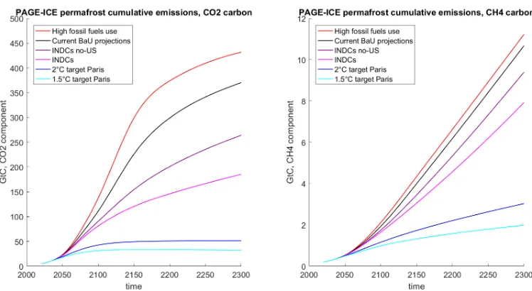
Figure 7. Cumulative carbon emissions from thawing land permafrost for the CO2 (left) and methane (right) components
under the six climate scenarios until year 2300. Mean values of 100,000 Monte-Carlo runs of PAGE-ICE. Units: GtC. Note the difference in the Y-axis scale between the plots.
The nonlinear Equation 1 and Equation 2 are solved analytically on each analysis period < < of the PAGE-ICE model using an improved technique described in the Supplementary Materials. Cumulative PAGE-ICE permafrost emissions (Figure 7) are higher than the SiBCASA emissions (Figure 1) due to the following two factors: (i) emissions-driven RCP scenarios in PAGE-ICE as opposed to concentration-driven RCPs in SiBCASA, and (ii) endogenous implementation of PCF in PAGE-ICE as opposed to uncoupled SiBCASA runs, which leads to higher GMST compared with the baseline and increases the permafrost emissions.
Emulator for nonlinear Sea Ice Albedo Feedback
Our new nonlinear emulator of SIAF builds on earlier studies with Earth system models (ESMs),22,23 and is calibrated using the latest ESMs simulation data for monthly mean sea ice extents under the RCP8.5 scenario until 2300, combined with standard insolation patterns with latitude and season. The calculations assume a circular sea ice cap centred at the North Pole during each month, cancelling out short-term spatial and temporal (daily and weekly) variations in the sea ice extent patterns across the Arctic Ocean. The insolation flux accounts for partial reflection of the shortwave radiation by the cloud cover.47 Monthly mean absorbed shortwave fluxes are aggregated to produce mean annual values of the RF north of 60N, which are then differentiated with respect to GMST trends over 30-year climatological windows using linear polynomial fitting to get average SIAF. A Savitzky–Golay filter with base period of 30 years and 2nd order polynomial interpolation is applied to obtain smooth time series for GMST and SIAF.
Figure 2 for the five ESMs as a function of GMST rise relative to pre-industrial levels.xviii They show a series of characteristic nonlinear transitions in the form of peaks and troughs associated with the varying pace of the loss of sea ice in the different months of a year relative to the seasonal changes in insolation patterns.22 These variations are linked not only with the insolation cycle itself, but with multiple other factors such as cross-latitudinal atmospheric and oceanic heat fluxes.
Most of the ESMs analysed show the initial increase in SIAF coinciding with the loss of the September sea ice, as well as distinct peaks occurring when the early summer and spring sea ice disappears, coinciding with strong insolation patterns. This behaviour is particularly pronounced in the MPI model. However, the relative magnitude of these effects varies significantly between the models, which is clear from Figure 2. For some models like MPI-ESM-LR and HadGEM2-ES, the near-term projections of SIAF driven by the loss of September sea ice are smaller than the projected peak associated with the loss of the spring sea ice. For other models like CNRM-CM5 and IPSL-CM5A-LR, the near-term projections of the albedo feedback are noticeably higher than those associated with the longer-term loss of the spring sea ice.
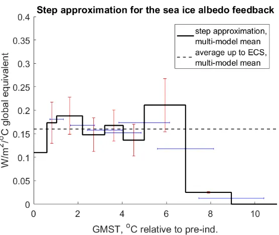
The SIAF emulator is based on a step-wise approximation with eight distinct eras (Figure 8). Both the approximated constant level of SIAF in each era , , (W/m2/°C), and the GMST level at which
transition between the given era and the next era occurs, , (°C from pre-industrial), are random variables calibrated according to the multi-model CMIP5 projections (error bars in Figure 8). The transition temperatures , between the eras are inferred from the SIAF plots based on the
approximate position of the inflection points that demarcate the regions around the peaks and the troughs. For each of the five ESM datasets analysed, only three dominant peaks in the albedo feedback are chosen, and piece-wise constant proxy values of the feedback , are introduced through
averaging of the actual feedback ( ) over the corresponding GMST eras , < < , .
The individual step-wise SIAF approximations from the five ESMs (represented by the , and ,
pairs) are then averaged according to the ranking system for the levels of misfit between the historic CMIP5 model simulations and the corresponding satellite data for the Arctic sea ice extent from two different satellite-derived datasets.51 The MPI-ESM-LR model achieved the best performance in each study, receiving the 100% ranking. The average rankings of the other models used in our study across the three regions are: 76% for CNRM-CM5 and 65% both for HadGEM2-ES and IPSL-CM5A-LR. Based on these rankings, normalised weighting factors of 0.19 for CNRM-CM5, 0.16 for HadGEM2-ES and IPSL-CM5A-LR, and 0.25 for MPI-ESM-LR-ctrl and MPI-ESM-LR-itd are derived. These weights are used to calculate the multi-model mean and variance of the individual , and , pairs to generate the corresponding probability ranges used in PAGE-ICE (Figure 8).
Figure 8. The multi-model mean step approximation of SIAF capturing the main nonlinear transitions between distinct eras (thick black line) according to the five ESMs analysed (Figure 2). The error bars show standard deviations for the “end of eras” temperatures (blue) and SIAF in each era (red). The average of SIAF up to 2xCO2 equilibrium climate sensitivity
(ECS) warming level is shown by the dashed line. The “end of eras” temperatures are correlated with one another, resulting in lower uncertainties in the widths of the eras (not plotted).
The cumulative “actual” RF (W/m2, global equivalent) due to SIAF measured from pre-industrial conditions is given by
( ) = , ( ′) ′ + , ( ′) ′,
Equation 3
where is the GMST rise relative to pre-industrial levels that falls into the -th sea ice era: , <
< , . If starts to decrease under a high abatement scenario such as RCP2.6, this formula is
reversible providing there is no hysteresis behaviour in the sea ice cover. The RF is then re-adjusted to be measured from the PAGE-ICE base year = 2015, and is projected on the analysis years of PAGE-ICE, with piece-wise linear interpolation with respect to GMST is used in between. For each analysis period < < characterised by the temperature range , < < , , the
interpolated SIAF-driven increase in the “actual” RF relative to the base year is given by
∆ ( ) = , + , ∙ − , − , , , = , ( ) ,
where , is SIAF in the analysis year , assumed to be constant on the subsequent analysis
period, and , and , are the values of the cumulative albedo forcing in the analysis year and the base year , both measured from pre-industrial conditions. In the absence of measurements prior to the satellite era, we use the available satellite data for the cumulative RF due to SIAF for the period between 1979 and 20088,27 to approximate
, = 0.11 W/m2.
The emulator also recognises that SIAF is implicitly included in the 2xCO2 equilibrium climate sensitivity parameter (ECS), which is central to modelling the greenhouse effect in IAMs like PAGE, DICE and FUND. Without acknowledging the baseline level of SIAF used in the ECS parameter, simply adding it to the anthropogenic RF would amount to double-counting. To date, none of the IAMs have had a temperature-varying ECS to reflect the nonlinear nature of planetary feedbacks such as SIAF. The ECS parameter in PAGE-ICE is based on specific 2xCO2 experiments in CMIP5 Earth system models (ESMs), resulting in multi-model mean equilibrium warming of around 2.8°C relative to pre-industrial levels.10 According to the ESM data analysed, the average level of SIAF for the hypothetical period between pre-industrial conditions and the mean 2xCO2 ECS warming of 2.8°C is = 0.165 W/m2/°C, which includes the cumulative base year RF estimate
, = 0.1 W/m2, and is in good
agreement with historic data.8,52,53 The implicit baseline assumption in IAMs to date has been that of a constant SIAF equal to . This is equivalent to the cumulative RF due to SIAF extrapolated linearly with the GMST anomaly − , relative to the base year for any future temperature levels :
∆ ( ) = ∙ − , .
Thus, the difference between the actual and linearly extrapolated “baseline” cumulative albedo forcing during the analysis period < < is
∆ ( ) = ∆ ( ) − ∆ ( )
= ∙ , − , + , − , ∙ , + , − ∙
≡ ∆ + ∆ ∙ ,
where we defined
∆ = ∙ , − , + , − , ∙ , , ∆ = , − .
As a result, the nonlinear correction to SIAF alters the governing equation for the GMST change in PAGE-ICE by adding extra terms to the total anthropogenic radiative forcing (RF) ( ), which modifies the 2xCO2 equilibrium climate sensitivity parameter ECS (°C) and the e-folding feedback response time FRT (yr) of the upper ocean layers to increased RF. For the analysis period < <
, the GMST equation becomes:
= 1
FRT ∙ ECS
ln 2 ∙ ( ) + ∆ − .
Equation 4
Here
ECS = ECS ∙ 1 − ECS
ln 2 ∆ , FRT = FRT ∙ 1 − ECS
ln 2 ∆
analytically during each analysis period < < using an improved technique described in the Supplementary Materials. The resulting difference between the actual and baseline cumulative RF from SIAF is plotted in Figure 5 for the six climate scenarios.
PAGE-ICE IAM
PAGE-ICE is based on the PAGE09 IAM.19,20 It includes several updates both in climate science and economics from IPCC AR510 and literature that followed, as well as several novel developments presented in this paper. The updates are summarised in the list below. Where necessary, they are described further in the Supplementary Materials and references therein.
The CO2 cycle in PAGE-ICE has been updated to give mean RF levels in 2100 that match closely with the definitions of the RCP scenarios: 2.61 W/m2 for RCP2.6, 4.84 W/m2 for RCP4.5, and 8.50 W/m2 for RCP8.5.xix PAGE and similar IAMs do not model natural climate variability, and therefore each Monte-Carlo run is deterministic in time. This allows us to work with Monte-Monte-Carlo generated probability distributions of multiple climatic and economic parameters in any fixed analysis year like 2100, as opposed to taking averages over the 30-year climatological windows (standard requirement for any climate model data with multiple natural variability cycles).
Generic updates:
• Adjusted analysis years starting with 2015 (base year), 2020, 2030, 2040, 2050, 2075, 2100, 2150, 2200, 2250 and 2300, allowing for a better representation of the essential long-term processes: permafrost emissions, winter sea ice decline and melting of the ice sheets.
• Updated base year (2015) data for the emissions, temperature, population, GDP-PPP, cumulative permafrost emissions and sea ice albedo feedback.
• Updated set of emissions (RCP) and socio-economic (SSP) scenarios paired according to the RCP-SSP compatibility conditions.29 The range of scenarios is in line with the multiple Paris Agreement pledges, and also covers the possibility of a reversal of climate policies in the US and globally.
• New high abatement scenario based on a ratcheted-up RCP2.6 pathway, in line with the 1.5°C target from Paris.
• New scenario in line with the current Paris pledges (INDCs), but without the US.
Climate science updates:
• Internal dynamic representation of the two nonlinear Arctic feedbacks: emissions from thawing land permafrost and changes in sea ice albedo. The dynamic emulators are based on simulations data from multiple state-of-the-art Earth system models and the SiBCASA ecosystems model run under the extended RCP8.5 and 4.5 scenarios until 2300.xx
• Adjusted TCR, FRT and ECS parameter ranges according to IPCC AR5 based on CMIP5 results.
• Revised CO2 cycle using a better closed form approximation for the solution of the main governing equation over the discrete analysis periods, as well as downscaled natural CO2 stimulation feedback.
• Improved GMST equation using a better closed form approximation for the solution of the main governing equation over the discrete analysis periods.
• CMIP5-based amplification factors for the regional temperatures.
• Changes in the implementation of the regional sulphate cooling. Sulphates now add to the global forcing and affect the regional temperatures implicitly through the CMIP5-based amplification factors. Their RF is not included in the regional temperature equation directly due to the complexity of climatic response to regional RFs, which requires regional climate sensitivities to be introduced.54 This level of complexity is beyond the philosophy of the climate emulator in the PAGE model that has been adopted so far.
• Approximately halved indirect sulphate cooling effect.
• Fat-tailed distribution for the sea level rise time lag (at the lower values end) to account for the possible collapse of the Greenland and West Antarctica ice sheets. 55,56,57
Economics updates:
• Significantly downscaled discontinuity sector that now accounts only for socio-economic tipping points such as pandemics, mass migration and wars (the catastrophic loss of the ice sheets has been moved to the fat-tailed distribution in the sea level rise module).
• Reduced tolerable temperature rise that gives no chance of a discontinuity. • Significantly decreased time constant of a discontinuity.
• Slightly increased mean and maximum default economic and non-economic impact at calibration temperature.
• Significantly modified uncertainty range for the “business as usual” emissions scenario, which is used as a reference point for calculating the abatement costs, roughly covering the range between RCP6.0 and RCP8.5.
• Alternative economic impact functions in line with the recent macro-econometric studies.36,58 • Revised marginal abatement cost (MAC) curves and technological learning rate (CO2 only).59,60
MPI-ESM-LR-itd model with improved sea ice thickness distribution
A technical description of the new MPI-ESM-LR-itd model and a brief analysis of its performance for Arctic sea ice relative to its predecessors is provided in Supplementary Materials.
Acknowledgements
Karcher and Rüdiger Gerdes. Dmitry Yumashev would like to thank Erasmus Research Institute of Management for additional funding.
We also acknowledge the World Climate Research Programme's Working Group on Coupled Modelling, which is responsible for CMIP, and we thank the climate modelling groups (listed in the Supplementary Materials) for producing and making available their model output. For CMIP the U.S. Department of Energy's Program for Climate Model Diagnosis and Inter-comparison provides coordinating support and led development of software infrastructure in partnership with the Global Organization for Earth System Science Portals.
Author contributions
DY, GW and CH conceived the research; DY and CH created the PAGE-ICE model; KS and EJ designed and ran SiBCASA permafrost simulations; KRC developed MPI-ESM-LR-itd model and ran sea ice simulations; FIS, KRC and KS processed netcdf data; DY developed and calibrated nonlinear permafrost and sea ice feedback emulators, performed PAGE-ICE runs and designed the graphics; All advised on the scientific and policy matters and wrote the paper.
Competing financial interests
The authors do not have competing financial interests.
Materials & Correspondence
All correspondence and material requests should be addressed to Dr. Dmitry Yumashev via [email protected].
References
1 Overland, J. E. et al. (2015) Surface Air Temperature (Arctic Report Card 2015); http://www.arctic.noaa.gov/report15/air_temperature.html.
2 Stroeve, J. C., Serreze, M. C., Holland, M. M., Kay, J. E., Malanik, J., & Barrett, A. P. (2012). The Arctic’s rapidly shrinking sea ice cover: a research synthesis. Climatic Change, 110(3), 1005-1027.
3 Wadhams, P. (2016). A Farewell to Ice. A Report from the Arctic. Allen Lane, London.
4 Van den Broeke, M. R., Enderlin, E. M., Howat, I. M., & Noël, B. P. (2016). On the recent contribution of the Greenland ice sheet to sea level change. The Cryosphere, 10(5), 1933.
5 Chadburn, S. E., Burke, E. J., Cox, P. M., Friedlingstein, P., Hugelius, G., & Westermann, S. (2017). An
observation-based constraint on permafrost loss as a function of global warming. Nature Climate Change, 7(5), 340-344.
6 Schaefer, K., T. Zhang, L. Bruhwiler, and A. P. Barrett (2011), Amount and timing of permafrost carbon release in response to climate warming, Tellus Series B: Chemical and Physical Meteorology, 63(2), pg. 165-180, DOI: 10.1111/j.1600-0889.2011.00527.x.
7 Schuur, E. A. G., McGuire, A. D., Schädel, C., Grosse, G., Harden, J. W., Hayes, D. J., ... & Natali, S. M. (2015). Climate change and the permafrost carbon feedback. Nature, 520(7546), 171-179.
8 Flanner, M. G., Shell, K. M., Barlage, M., Perovich, D. K., & Tschudi, M. A. (2011). Radiative forcing and albedo feedback from the Northern Hemisphere cryosphere between 1979 and 2008. Nature Geoscience, 4(3), 151. 9 Wadhams, P. (2012). Arctic ice cover, ice thickness and tipping points. AMBIO (Royal Swedish Acad. Sci), 41, 23-33.
10 Taylor, K. E., Stouffer, R. J., & Meehl, G. A. (2012). An overview of CMIP5 and the experiment design. Bulletin
of the American Meteorological Society, 93(4), 485-498.
11 Koven, CD, WJ Riley, and A Stern (2013), Analysis of Permafrost Thermal Dynamics and Response to Climate Change in the CMIP5 Earth System Models, J. Clim., 26(6), pg 1877-1900, DOI: 10.1175/JCLI-D-12-00228.1 12http://climateactiontracker.org/, accessed on 09 September 2017
13 Rockström, J., Gaffney, O., Rogelj, J., Meinshausen, M., Nakicenovic, N., & Schellnhuber, H. J. (2017). A roadmap for rapid decarbonization. Science, 355(6331), 1269-1271.
14 Figueres, C., Schellnhuber, H. J., Whiteman, G., Rockström, J., Hobley, A., & Rahmstorf, S. (2017). Three years to safeguard our climate. Nature, 546(7660), 593-595.
15
https://www.whitehouse.gov/the-press-office/2017/06/01/statement-president-trump-paris-climate-accord, accessed on 17 August 2017
16 Schellnhuber, H. J., Rahmstorf, S., & Winkelmann, R. (2016). Why the right climate target was agreed in Paris. Nature Climate Change, 6(7), 649-653.
17 O'Neill, B. C., Oppenheimer, M., Warren, R., Hallegatte, S., Kopp, R. E., Pörtner, H. O., ... & Mach, K. J. (2017). IPCC reasons for concern regarding climate change risks. Nature Climate Change, 7(1), 28-37.
18https://nsidc.org/news/newsroom/arctic-sea-ice-maximum-record-low-third-straight-year, accessed on 17 August 2017
19 Hope, C. (2006). The marginal impact of CO2 from PAGE2002: An integrated assessment model incorporating the IPCC's five reasons for concern. Integrated assessment, 6(1).
20 Hope, C. (2013). Critical issues for the calculation of the social cost of CO2: why the estimates from PAGE09 are higher than those from PAGE2002. Climatic Change, 117(3), 531-543.
21 Riemann-Campe, K., Kauker, F., Karcher, M., & Gerdes, R. (2017). Report on first simulations with improved parameterization in the climate model and the effect on the environmental variables to be coupled to the economic model of WP4, FP-7 Project ICE-ARC D2.51 report. European Commission.
22 Winton, M. (2006). Does the Arctic sea ice have a tipping point?. Geophysical Research Letters, 33(23). 23 Winton, M. (2008). Sea ice–albedo feedback and nonlinear Arctic climate change. Arctic sea ice decline:
Observations, projections, mechanisms, and implications, 111-131.
24 Hope, C., & Schaefer, K. (2016). Economic impacts of carbon dioxide and methane released from thawing permafrost. Nature Climate Change, 6(1), 56-59.
25 González-Eguino, M., & Neumann, M. B. (2016). Significant implications of permafrost thawing for climate change control. Climatic Change, 136(2), 381-388.
26 Kessler (2017) Estimating the economic impact of the permafrost carbon feedback, Clim. Change Econ., 08, 1750008. https://doi.org/10.1142/S2010007817500087.
27 González-Eguino, M., Neumann, M. B., Arto, I., Capellán-Perez, I., & Faria, S. H. (2017). Mitigation implications of an ice-free summer in the Arctic Ocean. Earth's Future, 5(1), 59-66.
28 Riahi, K., Rao, S., Krey, V., Cho, C., Chirkov, V., Fischer, G., ... & Rafaj, P. (2011). RCP 8.5 – A scenario of comparatively high greenhouse gas emissions. Climatic Change, 109(1-2), 33.
29 Riahi, K., Van Vuuren, D. P., Kriegler, E., Edmonds, J., O’neill, B. C., Fujimori, S., ... & Lutz, W. (2017). The shared socioeconomic pathways and their energy, land use, and greenhouse gas emissions implications: an overview. Global Environmental Change, 42, 153-168.
30https://tntcat.iiasa.ac.at/RcpDb/dsd?Action=htmlpage&page=welcome, accessed on 30 September 2017. 31 Burke, E. J., Ekici, A., Huang, Y., Chadburn, S. E., Huntingford, C., Ciais, P., ... & Krinner, G. (2017). Quantifying uncertainties of permafrost carbon–climate feedbacks. Biogeosciences, 14(12), 3051.
32 Tol, R.S.J., (2002), “New estimates of the damage costs of climate change, Part II: dynamic estimates.”, Environ. Resour. Econ., 21, 135-160.
33Warren, R., Hope, C., Mastrandrea, M., Tol, R., Adger, A., and Lorenzoni, I. 2006 ‘Spotlighting impacts functions in integrated assessment’ Research Report Prepared for the Stern Review on the Economics of Climate Change, Tyndall Centre Working Paper 91
34 Anthoff D, Nicholls RJ, Tol RSJ and Vafeidis AT, 2006 “Global and regional exposure to large rises in sea-level: a sensitivity analysis”. Working Paper 96, Tyndall Centre for Climate Change Research, Norwich, UK.
35 Stern, N. et al. 2007. The Economics of Climate Change: The Stern Review. Cambridge and New York: Cambridge University Press.
36 Burke, M., Hsiang, S. M., & Miguel, E. (2015). Global non-linear effect of temperature on economic production. Nature, 527(7577), 235-239.
38 Emmerson, C., & Lahn, G. (2012). Arctic opening: Opportunity and risk in the high north. LLoyd's.
39 Kriegler E, Hall JW, Held H, Dawson R, Schellnhuber HJ. (2009). Imprecise probability assessment of tipping points in the climate system. Proc. Natl. Acad. Sci. U. S. A. 106: 5041–5046.
40 Howard, P. (2014). Omitted damages: what’s missing from the social cost of carbon.
41 Cai, Y., Lenton, T. M., & Lontzek, T. S. (2016). Risk of multiple interacting tipping points should encourage rapid CO2 emission reduction.
42 Bettis, O. D., Dietz, S., & Silver, N. G. (2017). The risk of climate ruin. Climatic Change, 140(2), 109-118. 43 Schaefer, K., Zhang, T., Slater, A. G., Lu, L., Etringer, A. and Baker, I. (2009). Improving simulated soil temperatures and soil freeze/thaw at high-latitude regions in the Simple Biosphere/Carnegie-Ames-Stanford Approach model. J. Geophys. Res., 114, art. num F02021, doi:10.1029/2008JF001125.
44 Schaefer, K; and E. Jafarov (2016), A parameterization of respiration in frozen soils based on substrate availability, Biogeosciences, 13, 1991–2001, 2016,
www.biogeosciences.net/13/1991/2016/, doi:10.5194/bg-13-1991-2016
45 Hugelius, G., Tarnocai, C., Broll, G., Canadell, J. G., Kuhry, P., and Swanson, D. K. (2013) The Northern Circumpolar Soil Carbon Database: spatially distributed datasets of soil coverage and soil carbon storage in the northern permafrost regions, Earth Syst. Sci. Data, 5, 3–13, doi:10.5194/essd-5-3-2013.
46 Wei, Y; Liu, S; Huntzinger, DN; Michalak, AM; Viovy, N; Post, WM; Schwalm, CR; Schaefer, K; Jacobson, AR; Lu, C; Tian, H; Ricciuto, DM; Cook, RB; Mao, J; Shi, X (2014), The North American Carbon Program Multi-scale Synthesis and Terrestrial Model Intercomparison Project - Part 2: Environmental driver data, Geosci. Model Devel., (7)6, 2875-2893, DOI: 10.5194/gmd-7-2875-2014.
47 Kiehl, J. T., & Trenberth, K. E. (1997). Earth's annual global mean energy budget. Bulletin of the American
Meteorological Society, 78(2), 197-208.
48 Voldoire, A., Sanchez-Gomez, E., y Mélia, D. S., Decharme, B., Cassou, C., Sénési, S., ... & Déqué, M. (2013). The CNRM-CM5. 1 global climate model: description and basic evaluation. Climate Dynamics, 40(9-10), 2091-2121.
49Martin, G. M., Bellouin, N., Collins, W. J., Culverwell, I. D., Halloran, P. R., Hardiman, S. C., ... & O’Connor, F. M. (2011). The HadGEM2 family of Met Office Unified Model climate configurations, Geosci. Model Dev., 4, 723–757, doi: 10.5194.
50 Dufresne, J. L., Foujols, M. A., Denvil, S., Caubel, A., Marti, O., Aumont, O., ... & Bony, S. (2013). Climate change projections using the IPSL-CM5 Earth System Model: from CMIP3 to CMIP5. Climate Dynamics, 40(9-10), 2123-2165.
51 Riemann-Campe, K., Karcher, M., Kauker, F. & Gerdes, R. (2014). Results of Arctic ocean-sea ice downscaling runs validated and documented. FP7 Project ACCESS D1.51 report. European Commission. Url:
http://www.access-eu.org/modules/resources/download/access/Deliverables/D1-51-AWI-final.pdf .
52 Pistone, K., Eisenman, I., & Ramanathan, V. (2014). Observational determination of albedo decrease caused by vanishing Arctic sea ice. Proceedings of the National Academy of Sciences, 111(9), 3322-3326.
53 Cao, Y., Liang, S., Chen, X., & He, T. (2015). Assessment of Sea Ice Albedo Radiative Forcing and Feedback over the Northern Hemisphere from 1982 to 2009 Using Satellite and Reanalysis Data. Journal of Climate,
28(3), 1248-1259.
54 Shindell, D., & Faluvegi, G. (2009). Climate response to regional radiative forcing during the twentieth century. Nature Geoscience, 2(4), 294.
55 Golledge, N. R., Kowalewski, D. E., Naish, T. R., Levy, R. H., Fogwill, C. J., & Gasson, E. G. (2015). The multi-millennial Antarctic commitment to future sea-level rise. Nature, 526(7573), 421-425.
56 Hansen, J., Sato, M., Hearty, P., Ruedy, R., Kelley, M., Masson-Delmotte, V., ... & Velicogna, I. (2016). Ice melt, sea level rise and superstorms: evidence from paleoclimate data, climate modeling, and modern observations that 2 C global warming could be dangerous. Atmospheric Chemistry and Physics, 16(6), 3761-3812.
57 Le Bars, D., Drijfhout, S., and de Vries, H. (2017). A high-end sea level rise probabilistic projection including rapid Antarctic ice sheet mass loss. Environmental Research Letters, 12(4), 044013.
58 Dell, M., Jones, B. F., & Olken, B. A. (2012). Temperature shocks and economic growth: Evidence from the last half century. American Economic Journal: Macroeconomics, 4(3), 66-95.
59 Aldy, J. E., Pizer, W., Tavoni, M., Reis, L., Akimoto, K., Blanford, G., ... & McJeon, H. (2016). Economic tools to promote transparency and comparability in the Paris Agreement. Harward, US