Article
Massive RDF Query Processing Efficiently in Spark
Environment Based on Semantic Connection Set
Jiuyun Xu1,†,‡ , Chao Zhang1,‡
1 2 3 4 5 6 7 8 9 10 11 12 13
1 College of Computer and Communication Engineering, China University of Petroleum (East
China),Tsingdao 266580, China;[email protected](X.J.);[email protected](C.Z.) * Correspondence:[email protected];
‡ These authors contributed equally to this work.
Abstract:ResourceDescriptionFramework(RDF)isadatarepresentationformatoftheSemanticWeb,
anditsdatavolumeisgrowingrapidly.Cloud-basedsystemsprovidearichplatformformanaging
RDFdata.However,thedistributedenvironmenthasperformancechallengeswhenitisprocessing
withRDFqueriesthatcontainmultiplejoinoperations,suchasnetworkreshuffle,memoryoverhead.
Togetoverthesechallenges,thispaperproposedaspark-basedRDFqueryarchitecture,whichis
basedonSemanticConnectionSet(SCS).Firstofall,thisspark-basedqueryarchitectureadoptsthe
mechanismofre-partitioningclassdatabasedonverticalpartitioning,whichcanreducememory
overheadandfastindexdata. Secondly,amethodforgeneratingqueryplansbasedonsemantic
connectionsetsisproposedinthispaper.Inaddition,statisticsandbroadcastvariableoptimization
strategiesareusedtoreduceshufflinganddatacommunicationcosts.Theexperimentofthispaperis
basedonthelatestSPARQLGXonthesparkplatformRDFsystem,twosyntheticbenchmarksare
usedtoevaluatethequery.Theexperimentresultillustratesthattheproposedapproachinthispaper
ismoreefficientindatasearchthanSPARQLGX.
Keywords:RDF;SemanticWeb;BasicGraphPattern;DistributedSPARQLQueryProcessing;Spark
14
1. Introduction 15
With the development of Web 3.0 and knowledge graph, the data represented by the Resource
16
Description Framework(RDF)[1] is increasing rapidly. There are many reasons for this phenomenon
17
,such as search engine like Google add semantics to web pages to improve query accuracy .In addition,
18
a growing number of communities driven projects are constructing large knowledge bases with billions
19
of facts in many domains to implement more useful applications, for example DBpedia, Probase and
20
so on.
21
SPARQL(SPARQL Protocol and RDF Query Language)[2] recommended by W3C is the main
22
query language for RDF data. The SPARQL query sentences contain a cluster of triple patterns. The
23
system searches triple that match on the conditions. One variable can be in multiple triple patterns,
24
the system has to check all the conditions about a variable.
25
During the past decade, most traditional RDF management system executed in a single machine
26
can not handle large-scale RDF data and answer complex query. But to handle large-scale RDF
27
data, several methods are presented in terms of storage strategies and query strategies, such as
28
RDF-3X[3],Hexastore[4],SW-Store[5]. Now industry dealing with large-scale data storage usually
29
considers a distributed environment by partitioning RDF data in many compute nodes and evaluating
30
queries in a distributed fashion,e.g., Spark, can be used [6]. SPARQL query is decomposed into multiple
31
subqueries that are evaluated by each node independently. Since data is distributed, the nodes may
32
need to exchange intermediate results during query evaluation. Consequently, queries with large
33
intermediate results incur high communication cost, which is detrimental to the query performance.
34
In this paper, we demonstrate that the system is mainly consider querying for large-scale RDF
35
data efficiently in the distributed environment. The main problem are considered about the following
36
two points:
37
• Storage part, how to reduce memory overhead through partition and index data and achieve a
38
balance between data preprocessing and fast indexing. Different storage and access methods
39
directly affect the efficiency of the query.
40
• Query part, how to reduce SPARQL query processing costs and communication costs. The
41
SPARQL query processing can be transformed to the problem of iterative matching and joining
42
of sub-queries.
43
The contributions of this paper are summarized as follows:
44
• Unlike existing most systems that use a set of permutations of (S,P,O) indexes, we introduce a
45
VP-based storage schema for management massive RDF data by further partitioningrdf:type
46
predicate based on Vertical Patitioning(VP)[7]. The strategy is designed to minimize the size
47
of the input data to achieve the goal of reducing memory overhead and supporting the fast
48
indexing.
49
• Cost estimation and optimization query strategies are presented in this paper. Semantic
50
connection set generates query plan and uses broadcast variables method to avoid lots of
51
communication costs. These optimizations ensure high performance for our system.
52
• We perform an experimental evaluation by comparing this system and current state-of-the-art
53
SPARQLGX that query RDF data on the Spark platform. We test the performance of current
54
works over LUBM[8] datasets and Watdiv[9] datasets via standard benchmark queries. The
55
results prove the effectiveness of this system.
56
The rest of this paper is organized as follows: section2presents the related work. section3mainly
57
introduces basic knowledge RDF data and SPARQL queries. The section4mainly introduces system
58
architecture. The section5mainly introduces data preparation. The section6mainly introduces query
59
processing. The section7is the experimental analysis, with latest distributed query SPARQLGX system
60
for comparison. Finally, we conclude in section8.
61
2. Related Work 62
In recent years, many rdf systems capable of evaluating sparql queries have been developed.
63
These stores can be divided in two categories: centralized systems and distributed ones, running
64
on single machine or on a computing cluster. RDF-3x[3] creates an exhaustive set of indexes for
65
all RDF triple permutations and aggregates indexes for subsets, resulting in a total of 15 indexes
66
stored in compressed clustered B trees. Besides, it also employs additional indexes to collect statistical
67
information for pairs and stand-alone entities to eliminate the problem of expensive self-joins and
68
provides great performance improvement. However, storing all the indexes is expensive and query
69
efficiency highly depends on the amount of main memory. VP is another representation for RDF
70
data proposed by SW-Store[5]. The triples table is vertically partitioned into n tables, where n is the
71
number of distinct predicates. A two columns table is created for each predicate where a row is a pair
72
of subject-object values connected through the predicate. It provides good performance for queries
73
with bounded predicates. However, it does not consider special class predicates to achieve further
74
fine-grained data. HadoopRDF[10] partitions the input RDF graph to create a pos or pso index. Then
75
the predicate files are splitted into smaller files according to the type of objects. It performs the SPARQL
76
query by a serious of iterative MapReduce jobs, each of which implements a join between two TPs on
77
a variable. However, its use of greedy algorithms to reduce the number of MapReduce connections
78
required for each step raises many unnecessary intermediate results. H2RDF+[11] stores and indexes
RDF data in HBase. Then it implements MapReduce-based multi-way Merge and ,Sort-Merge join
80
algorithms to process SPARQL query. However, since each MapReduce job requires a given input
81
and output, it will take a lot of time to read and write IRs in HBase. SPARQLGX[12] is designed to
82
leverage existing Hadoop infrastructures for evaluating sparql queries. It uses VP to process data and
83
then store it in HDFS. In addition, the system’s query optimization statistics is to read all the data for
84
statistics, which ignores the query information only needs to calculate the size of the query associated
85
data. S2RDF[13] is built on Spark and uses its SQL interface to execute SPARQL queries. Its main goal
86
is to address efficiently all SPARQL query shapes. Its data layout corresponds to the VP approach.
87
So-called ExtVP relations are computed at data load-time using semi-joins, to limit the number of
88
comparisons when joining triple patterns. Considering query processing, each triple pattern of a query
89
is translated into a single SQL query and the query performance is optimized using the set of statistics
90
and additional data structures computed during this pre-processing step. but, the data pre-processing
91
step generates an important data loading overhead which might be up to 2 orders of magnitude larger
92
than our solution.
93
3. Preliminary 94
3.1. RDF 95
RDF is the W3C recommended standard model for data interchange on the Web. It helps search
96
engines to understand the relation of these resources. The underlying structure of the data model
97
is simple and flexible. Any expression in RDF is a collection of triples , including a subject(s),a
98
predicate(p) and an object(o). Subject is a fact or a class of resources. Predicate denotes relationship
99
associated between fates or classes, and object is an entity,a class, or a literal value.
100
According this structure, the RDF dataset represents the information of the semantic web as a
101
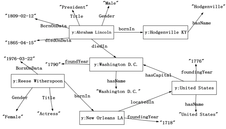
directed graph. RDF graph is a finite set of RDF triples. Figure1shows an example of RDF graph.
102
Ellipse nodes represent resource, edges represent relationship, and rectangular nodes represent literal
103
values.
y:Abraham Lincoln
"President" "Male"
"1809-02-12"
"1865-04-15"
y:Hodgenville KY
"Hodgenville"
y:Reese Witherspoon
y:United States
y:New Orleans LA y:Washington D.C.
"Washington D.C." "1790"
"1976-03-22"
"Female" "Actress"
"1718"
"United States" "1776" Gender
Title
BornOnData
diedOnData
diedIn
hasName foundYear
BornOnData
Gender Title bornIn
locatedIn hasName
foundingYear
foundingYear hasCapital bornIn
hasName
3.2. SPARQL 105
SPARQL is the W3C recommended query language for RDF. Its syntax is similar to the syntax
106
of a relational query. SPARQL query usually contains multiple triple patterns (TPs). A set of triple
107
patterns forms a basic graph pattern(BGP). Each tuple contains variables represented as ?v, then a
108
group of queries corresponds to a group of n subqueries, each subqueries contains a triple, according
109
to relevant variable of the triple can query information. We summarize the query process as follows:
110
compute binding values for every TP, implement joins intermediate result, and build the final result of
111
the query. For example, the SPARQL query statement is shown in Figure2.
Figure 2.SPARQL Query Statement 112
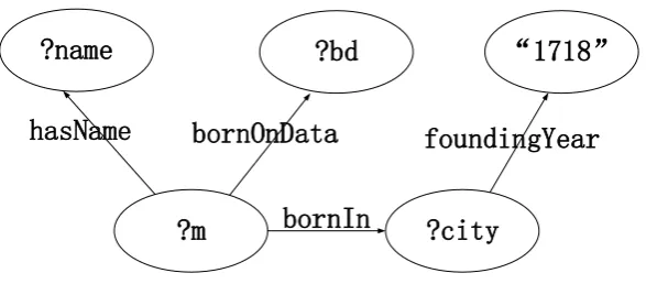
Corresponding to above SPARQL query, the SPARQL query graph is shown in Figure3.
?name
?m
?bd
?city
“1718”
hasName
bornOnData
bornIn
foundingYear
Figure 3.SPARQL Query Graph 113
4. System Architecture 114
In this section, we will introduce the system architecture. For the massive RDF dataset, a single
115
node is difficult to support access data. Distributed system can precede of the low cost, fault tolerance,
116
stability, scalability. Therefore, we propose a system for querying large-scale RDF data based on
117
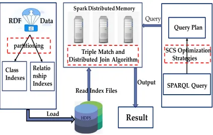
Spark. Figure4shows the architecture of the our system. On the whole, the system structure includes
118
four aspects: data preparation module, persistent data module, query parser module and distributed
119
processing module.
Spark Distributed Memory
HDFS
Triple Match and
Distributed Join Algorithm
Read Index Files
RDF
Data
partitioning
Class
Indexes
Relatio
nship
Indexes
Query
Result
SPARQL Query
Query Plan
SCS Optimization
Strategies
Output
Load
Figure 4.System Architecture
In this system architecture, the data preparation module is designed to convert RDF data in the
121
form of XML into n-triples format, further divide classes and relationships based on vertical partition,
122
and generate relational index files and class index files. The persistent data module is responsible for
123
loading the index files divided by the above modules into HDFS. The details of the above two modules
124
are described in section5. The query parser module is used to generate a query plan based on the SCS
125
optimization strategy, including the triple patterns join order, and the broadcast variable information.
126
Based on the parsing information, we loaded the corresponding index files from HDFS into Spark
127
distributed memory and persisted them. The distributed processing module performs local matching
128
and iterative join operation according to the query plan and finally generates the query result. More
129
details will be introduced in section6.
130
5. Data Partitioning 131
Data layout plays a significant role for efficient SPARQL queries in a distributed environment.
132
The most straight forward representation of RDF in a relational model is a named triple table with
133
three columns, containing one row for each RDF triple(s,p,o). Generally for efficient query, it will be
134
accompanied by several indexes over some or six triple permutations as query evaluation essentially
135
boils down to a series of a join on this large table. For example, well-known system RDF-3X[3], this
136
system creates a set of indexes on RDF data. However, this indexing approach can take up several
137
times the storage space. Since the size of its indexes files is still large which will lead to the overhead
138
of memory. Many cloud-based systems [14] use VP that it introduced by Abadi et al in [7]. such
139
as [15],[13],[12]. It uses a two-column table instead of three-column for every RDF predicate. The
140
predicate is the name of the file, subject and object is the two columns of data in the file. In the RDF
141
data, the number of predicates is generally small. So when we retrieve a triple containing this predicate,
142
we can quickly find the corresponding index file.
Different data partitioning and access methods directly affect the efficiency of the query. In this
144
paper, we propose several design goals:
145
• Reduce the time required to convert raw data to target data while ensuring finer-grained
146
partitioning schema.
147
• Reduce the size of input data to avoid the overhead of memory.
148
• Fasts retrieval of related index files.
149
0 20000 40000 60000 80000 100000 120000
Number of predicates
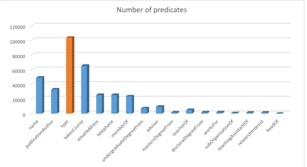
Figure 5.Sample Number of Each Predicates
Take the LUBM benchmark as an example, which contains 355,823 triples. Figure5shows the number
150
and proportion of each predicate.We can see that the number of predicate ofrdf:typeis at most.
151
Therefore, further partitioning of this predicate will speed up the related indexes. Thus, we introduce
152
a storage schema for management massive RDF data by further partitioningrdf:typepredicate based
153
on VP. In general, VP uses a two-columns table for every RDF predicate, e.g.workfor(s,o). On this
154
basis, we further divide the triples with predicate of type. We divide them into small class files based
155
on the triple’s object representing a specific class. The instances belonging to the same class are stored
156
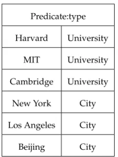
in corresponding class index files. Object will be the name of the file. Table123shows the partitioning
157
of the type predicate into smaller index files(class index files). We stored the partitioned data into the
158
file system of Hadoop(HDFS)[16].
159
This data partitioning method allows the system to quickly match each triple pattern by selecting
160
the relevant small index file when executing the SPARQL query, which reduces the cost of reading
161
indexes and avoids the overhead of memory. In addition, the data compression performance is
162
excellent because the data is not stored in the triple form. We will save two-thirds of the RDF data
163
storage space.
164
6. Query Processing 165
As important as data partitioning, the strategies for processing SPARQL query are focused on
166
searches. In this section, we will introduce the cost estimation, and then triple patterns matching based
167
on Spark, and finally the query optimization strategies based on the cost estimation.
Predicate:type
Harvard University
MIT University
Cambridge University
New York City
Los Angeles City
Beijing City
Table 1.Sample of Predicate Type
Indexname:University Harvard
MIT Cambridge Table 2.Spilt1
Indexname:City New York Los Angeles
Beijing Table 3.Spilt2
6.1. Cost Estimation 169
From the above introduction, we can divide SPARQL query into two aspects: triple patterns matching and join intermediate results. So we define the first part as parse TPs, and the second part as join IRs. The cost of parsing TP includes the cost of reading related index files and matching TP. The cost of joining IRs includes shuffle communication costs and computing costs.
Cost=
n
∑
i=1
Parser(TPi) + n
∑
j=2
Join IRj−1,Match(TPi) (1)
Parse(TPi) =Read(TPi) +Match(TPi) (2)
Join(IR1,IR2) =Shu f f le(IR1,IR2) +Compute(IR1,IR2) (3)
IRi =
(
join(IRi−1,Match(TPi)), 2≤i≤n
Match(TPi), i=1
(4)
Where,
170
n = number of TP in SPARQL query.
171
Read(TPi) = load the relevant index file.
172
Match(TPi) = the result of matching TPi.
173
shuffle(IR1,IR2) = the size of data that needs to be moved in a distributed environment.
174
compute(IR1,IR2) = the size of data required to implement the join operation.
175
IRi= the IR of TPi.
176
Equation1estimates the overall cost of a SPARQL query. Equation2specifically estimates the cost of
177
parsing a triple pattern. Equation3represents the cost of implementing the join operation. Equation4
represents iterative computation of IRs. Therefore, from the perspective of total cost estimation, we
179
reduce the cost of loading data and matching TP through data partitioning. In addition, the cost of
180
joining is roughly proportional to the size of their matching result, so we can reduce the connection
181
cost by reducing the size of intermediate results and data communication costs.
182
6.2. Triple Patterns Matching 183
Spark[17] is a general-purpose in-memory cluster computing system that runs on Hadoop and
184
can process data from any Hadoop data source. Compared to map-reduce-based systems[18][19][20],
185
our SPARQL query systems based on Spark does not need to write intermediate results back to disk,
186
which causes a large number of disk I/O problems. Instead, they are cached in memory to avoid
187
disk I/O costs. In the example query showed in preliminary section 2, the BGP contains a set of
188
triple patterns. For this, The goal of query is to compute the bindings for all variable. As every TP
189
can be regarded as a sub-query, the problem of SPARQL query processing can be transformed to the
190
problem of triple patterns matching and iterative joining of sub-queries. Calculating the binding for
191
all variables means matching the variables in each triple pattern separately. Jena ARQ[21] is used to
192
parse SPARQL query to generate the corresponding triple patterns. Each triple contains three parts of
193
the subject, predicate, and object, including constants and variables, in which the variables contain ?
194
of special characters. When the value of the predicate is constant, we can obtain the relevant data of
195
each tuple according to our previous data partitioning strategy, and further filtering related data based
196
on whether the subject and object are constants and using common operators in Spark. Then we will
197
count the size of the matching result and use it in the next optimization strategy.
198
For example, in the former section 2 showed, the tuple {?city <foundingYear> "1718" .}, where
199
f oundingYearand 1718 are constants, we read the index file in the file system based on the fact that
200
the predicate f oundingYear, and then filter the related data just read based on the fact that object is
201
1718. After each triple pattern is matched to the result, iterative join according to query plan we will
202
describe in detail in the query optimization section.
203
Algorithm 1:Triple Matching Algorithm
Input:tp:(s,p,o)
Output:IR
1 ifp is constantthen 2 ifp is rdf:typethen
3 ifo is constantthen
4 tq=spark.textFile(o.txt); 5 else
6 tq=spark.textFile(p.txt);
7 else
8 tq=spark.textFile(p.txt);
9 else
10 tq=spark.textFile(D.txt);
11 ifs is constantthen
12 tq=tq.Filtercase(s,o) =>s.equals(constant);
13 size=tq.count;
14 ifo is constantthen
15 tq=tq.Filtercase(s,o) =>o.equals(constant); 16 size=tq.count;
17 new IR(tq,size); 18 returnIR
The triple matching algorithm is showed in algorithm1. In summary, line 1 through line 8
205
represent the case where the predicate is constant, and 9 through 10 represent the case where the
206
predicate is variable. Line 2 through line 6 consider the special case where the predicate is type. Line
207
11 through line 16 represent triples that are filtered by the given subject or object.
208
6.3. Query Optimization 209
In the cost estimation, we mentioned reducing the cost of join by reducing the size of the results in
210
the process and data communication. Due to BGP query contains multiple triples, we join them based
211
on shared variables. But in the process of query, different connection order has different efficiency on
212
query result. Therefore, we propose a SCS optimization strategy to generate the join order in the RDF
213
query.
214
6.3.1. Semantic Connection Set
215
The join order of SPARQL sub-queries has a significant impact on query performance, so the
216
semantic connection set(SCS) optimization method needs to be built. The SCS contains multiple
217
intermediate results(IRs) obtained after multiple TP matches, and then sorted in ascending order
218
according to the size of IR. The size of IRs in the initial set is statistical in subsection6.2, and then
219
the two smaller intermediate results that contain common variables are selected to join first, and the
220
generated results are added to the set. Remove the previously connected IRs and sort by size. Iterate
221
join through the intermediate results until only one result remains in the set, which is the final result of
222
the SPARQL query. Finally, we return the columns of interest to the user. We use the SCS method to
223
generate an optimized query plan to improve the performance of RDF queries. This approach will
224
reduce the intermediate result size to save I/O and reduce the total number of connection comparisons
225
to save CPU.
226
As shown in algorithm2, the line 2 represents the smallest IR from the set of semantic connection.
227
From line 3 to line 6 indicate that the matching results in the set that contains same variable and the
228
smallest IR are extracted. Lines 8 through 10 represent the two result sets that implement the join
229
operation and remove it from the set, after which the join result is loaded into the connection set.
230
Algorithm 2:SCS Algorithm
Input:List(IRs)
Output:Query Result
1 whilelist.size>1do
2 IR1=list.minby(.getSize); 3 canJoin=list.f ilter(rdd=>
rdd.ne(IR1)&&rdd.getVarSet.intersect(IR1.getVarSet).nonEmpty); 4 ifcanjoin.isEmptythen
5 print(”can not join into one”);
6 IR2=canjoin.minby(.getSize);
7 broadcast(IR2); 8 join= IR1.join(IR2); 9 list.delete(IR1,IR2); 10 list.add(join);
11 QueryResult=list.head.getTriple;
12 returnQuery Result
231
In addition, In line 7 of the algorithm, we use the method of broadcasting variables to reduce the
232
network cost in data communication. When doing the join intermediate result operation, we compress
233
the data of the smaller result setAand broadcast it to the node of the result setBand make a local
234
connection. This operation can reduce a certain amount of network communication cost caused by
235
data shuffle.
7. Experiments 237
In this section, we will describe the performance evaluation of the SCS. The experiment
238
is implemented on a small cluster with five machines. Each node with an Inter Xeon E5-2670
239
CPU @2.6GHz,4 cores, 16GB RAM running Ubuntu 16.04.5 LTS with the software Scala2.11.1[22],
240
Hadoop2.7.3 and Spark2.1.0. A variety of experimental data sets are proposed in [23] .In our
241
experiment, we compare the presented systems using two synthetic benchmarks: LUBM [8] and
242
Watdiv[9].Test dataset are WatDiv10M and LUBM100. WatDiv10M contains 10 million triple data
243
and LUBM100 contains 12 million triple data. We test the query time over the datasets above via the
244
standard Watdiv and LUBM queries to prevent some queries absence of a final result. In addition, we
245
classify queries into three types:linear (L), star (S), snowflake (F).
246
Our system runs in a distributed environment, and the latest RDF distributed query engines
247
based on Spark are S2RDF and SPARQLGX. [12] shows that SPARQLGX performs better in both the
248
preprocessing and query stages than S2RDF. In addition, the SPARQLGX system adopts the method
249
of VP similar to our system, so our experimental results are mainly considered for comparison with
250
it.Since our system only further divides type predicate compared with SPARQLGX in data partitioning,
251
the comparison between the two in data preprocessing can be ignored. We compare the two systems
252
in terms of response time for the three query types.
253
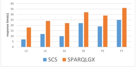
For dataset LUBM100, our experiments run standard queries on the data with 12 million tuples
254
and results are shown in figure6.
255
0 5 10 15 20 25 30 35 40
L3 L5 S3 S5 F5 F7
resp
o
n
se
ti
m
e(
s)
SCS
SPARQLGX
Figure 6.Query Time over LUBM100
the numbers after the letters, such as L3, represent a triple pattern in a sparql query that contains
256
the corresponding numbers. The performance comparison between our system and SPARQLGX is
257
shown in Figure6, we can see that our system outperforms the comparison system in query response
258
time regardless of the query type or the number of triples contained. This can be attributed to the
259
following two reasons: i)finer-granined partitioning schema. Our system matches a Tp by inputting a
260
smaller index file than sparqlgx; ii)optimal query plan. Compared with sparqlgx, the query plan made
261
by our system and the method of broadcasting variables can avoid a lot of communication costs.
262
For WatDiv10M, our experiments run queries on the data with 10 million tuples and results are
263
shown in figure7.
264
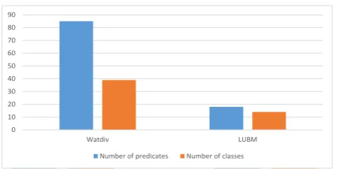
As shown in Figure7, we can find that our system in all the types of standard queries is better
265
efficiency than SPARQLGX. The difference between LUBM and Watdiv data sets is the number of
266
predicates, where LUBM contains 17 different predicates and Watdiv 86 different predicates. In this
267
system, the data with predicaterdf:typeis further divided, as shown in the Figure8, in which Watdiv
268
divides more index files than LUBM. Therefore, when doing an evaluation query under a data set of
0 5 10 15 20 25 30 35 40
L3 L5 S3 S5 F5 F7
re
spo
n
se
tim
e(s)
SCS
SPARQLGX
Figure 7.Query Time over Watdiv10M
the same size, the time required to read the index files divided by the LUBM dataset is likely to be
270
greater than the index files divided by the Watdiv dataset.
271
0 10 20 30 40 50 60 70 80 90
Watdiv LUBM
Number of predicates Number of classes
Figure 8.Number of Predicates category
8. Conclusion 272
In this paper, we introduce the SCS, RDF query processing engine based on Spark. We present a
273
schema for further partitioning data with predicate ofrdf:typebased on VP to avoid the overhead
274
of memory and speed up indexing. Then the intermediate results size affects the performance of the
275
system, so a semantic connection set method is built to handle the query process in a distributed
276
environment. We propose a cost model and other optimization strategies to specify the query order to
277
speed up the response time. For future work, we will increase the filtering of extraneous RDF data to
278
further reduce the amount of data read and investigate more efficient query join algorithm.
279
Author Contributions:CZ conceived the idea. JX conducted the analyses. All authors contributed to the writing 280
and revisions. All authors read and approved the final manuscript. 281
Conflicts of Interest:The authors declare no conflict of interest. 282
The following abbreviations are used in this manuscript: 284
RDF Resource Description Framework SCS Semantic Connection Set
SPARQL SPARQL Protocol and RDF Query Language VP Vertical Partitioning
TPs Triple Patterns BGP Basic Graph Pattern IRs Intermediate Results
L Linear
S Star
F Snowflake
285
References 286
1. Hayes, P. RDF Semantics. Recommendation2004. 287
2. Prud, E.; Seaborne, A.; others. Sparql query language for rdf2006. 288
3. Neumann.; Thomas.; Weikum.; Gerhard. The RDF-3X engine for scalable management of RDF data. Vldb 289
Journal2010,19, 91–113. 290
4. Weiss, C.; Karras, P.; Bernstein, A. Hexastore: sextuple indexing for semantic web data management. 291
Proceedings of the Vldb Endowment2008,1, 1008–1019. 292
5. Abadi, D.J.; Marcus, A.; Madden, S.R.; Hollenbach, K. SW-Store: a vertically partitioned DBMS for 293
Semantic Web data management. Vldb Journal2009,18, 385–406. 294
6. Agathangelos, G.; Troullinou, G.; Kondylakis, H.; Stefanidis, K.; Plexousakis, D. RDF Query Answering 295
Using Apache Spark: Review and Assessment. 2018 IEEE 34th International Conference on Data 296
Engineering Workshops (ICDEW), 2018. 297
7. Abadi, D.J.; Marcus, A.; Madden, S.R.; Hollenbach, K. Scalable semantic web data management using 298
vertical partitioning. Proceedings of the 33rd international conference on Very large data bases. VLDB 299
Endowment, 2007, pp. 411–422. 300
8. Guo, Y.; Pan, Z.; Heflin, J. LUBM: A benchmark for OWL knowledge base systems.Social Science Electronic 301
Publishing2005,3, 158–182. 302
9. Aluç, G.; Hartig, O.; Özsu, M.T.; Daudjee, K. Diversified Stress Testing of RDF Data Management Systems. 303
2014. 304
10. Husain, M.; McGlothlin, J.; Masud, M.M.; Khan, L.; Thuraisingham, B.M. Heuristics-based query 305
processing for large RDF graphs using cloud computing. IEEE Transactions on Knowledge and Data 306
Engineering2011,23, 1312–1327. 307
11. Papailiou, N.; Konstantinou, I.; Tsoumakos, D.; Karras, P.; Koziris, N. H 2 RDF+: High-performance 308
distributed joins over large-scale RDF graphs. IEEE International Conference on Big Data, 2013. 309
12. Graux, D.; Jachiet, L.; Geneves, P.; Layaïda, N. Sparqlgx: Efficient distributed evaluation of sparql with 310
apache spark. International Semantic Web Conference. Springer, 2016, pp. 80–87. 311
13. Schätzle, A.; Przyjaciel-Zablocki, M.; Skilevic, S.; Lausen, G. S2RDF: RDF querying with SPARQL on spark. 312
Proceedings of the VLDB Endowment2016,9, 804–815. 313
14. Kaoudi, Z.; Manolescu, I. RDF in the clouds: a survey. The VLDB Journal—The International Journal on Very 314
Large Data Bases2015,24, 67–91. 315
15. Schätzle, A.; Przyjaciel-Zablocki, M.; Hornung, T.D.; Lausen, G. PigSPARQL: a SPARQL query processing 316
baseline for big data. Th International Conference on Posters & Demonstrations Track, 2013. 317
16. Shvachko, K.; Radia, S.; Cox, A.L. The hadoop distributed file system. IEEE Symposium on Mass Storage 318
Systems & Technologies, 2010. 319
17. Zaharia, M.; Chowdhury, M.; Franklin, M.J.; Shenker, S.; Stoica, I. Spark: cluster computing with working 320
sets. Usenix Conference on Hot Topics in Cloud Computing, 2010. 321
18. Rohloff, K.; Schantz, R.E. High-performance, massively scalable distributed systems using the MapReduce 322
software framework: the SHARD triple-store. Programming Support Innovations for Emerging Distributed 323
19. Zhang, X.; Chen, L.; Wang, M. Towards efficient join processing over large RDF graph using mapreduce. 325
International Conference on Scientific & Statistical Database Management, 2012. 326
20. Zhang, X.; Lei, C.; Tong, Y.; Min, W. EAGRE: Towards scalable I/O efficient SPARQL query evaluation on 327
the cloud. IEEE International Conference on Data Engineering, 2013. 328
21. Mcbride, B. Jena: a semantic Web toolkit. IEEE Internet Computing2002,6, 55–59. 329
22. Weston, T. The Scala Language2018. 330
23. Abdelaziz, I.; Harbi, R.; Khayyat, Z.; Kalnis, P. A survey and experimental comparison of distributed 331