Application of Differential and Polarimetric Synthetic Aperture Radar (SAR) Interferometry for Studying Natural Hazards

(1)

Scholarship@Western

Electronic Thesis and Dissertation Repository

9-24-2013 12:00 AM

Application of Differential and Polarimetric Synthetic Aperture

Radar (SAR) Interferometry for Studying Natural Hazards

Samira Alipour

The University of Western Ontario

Supervisor Dr. Kristy Tiampo

The University of Western Ontario Graduate Program in Geophysics

A thesis submitted in partial fulfillment of the requirements for the degree in Doctor of Philosophy

Follow this and additional works at: https://ir.lib.uwo.ca/etd

Part of the Other Earth Sciences Commons, and the Tectonics and Structure Commons

Recommended Citation Recommended Citation

Alipour, Samira, "Application of Differential and Polarimetric Synthetic Aperture Radar (SAR)

Interferometry for Studying Natural Hazards" (2013). Electronic Thesis and Dissertation Repository. 1673. https://ir.lib.uwo.ca/etd/1673

This Dissertation/Thesis is brought to you for free and open access by Scholarship@Western. It has been accepted for inclusion in Electronic Thesis and Dissertation Repository by an authorized administrator of

(2)

INTERFEROMETRY FOR STUDYING NATURAL HAZARDS

(Thesis format: Integrated-Articles)

by

Samira Alipour

Graduate Program in Geophysics

A thesis submitted in partial fulfillment

of the requirements for the degree of

Doctor of Philosophy

The School of Graduate and Postdoctoral Studies

The University of Western Ontario

London, Ontario, Canada

(3)

ii

Abstract

In the following work, I address the problem of coherence loss in standard Differential

Interferometric SAR (DInSAR) processing, which can result in incomplete or poor quality

deformation measurements in some areas. I incorporate polarimetric information with

DInSAR in a technique called Polarimetric SAR Interferometry (PolInSAR) in order to

acquire more accurate and detailed maps of surface deformation.

In Chapter 2, I present a standard DInSAR study of the Ahar double earthquakes (Mw=6.4

and 6.2) which occurred in northwest Iran, August 11, 2012. The DInSAR coseismic

deformation map was affected by decorrelation noise. Despite this, I employed an advanced

inversion technique, in combination with a Coulomb stress analysis, to find the geometry and

the slip distribution on the ruptured fault plane. The analysis shows that the two earthquakes

most likely occurred on a single fault, not on conjugate fault planes. This further implies that

the minor strike-slip faults play more significant role in accommodating convergence stress

accumulation in the northwest part of Iran.

Chapter 3 presents results from the application of PolInSAR coherence optimization on

quad-pol RADARSAT-2 images. The optimized solution results in the identification of a

larger number of reliable measurement points, which otherwise are not recognized by the

standard DInSAR technique. I further assess the quality of the optimized interferometric

phase, which demonstrates an increased phase quality with respect to those phases recovered

by applying standard DInSAR alone.

Chapter 4 discusses results from the application of PolInSAR coherence optimization from

different geometries to the study of creep on the Hayward fault and landslide motions near

Berkeley, CA. The results show that the deformation rates resolved by PolInSAR are in

agreement with those of standard DInSAR. I also infer that there is potential motion on a

secondary fault, northeast and parallel to the Hayward fault, which may be creeping with a

(4)

iii

Finally, discussions on the application of the PolInSAR technique and the geophysical

implications of the standard DInSAR study are presented, with suggestions for future work,

in the conclusions.

Keywords

Differential Interferometric Synthetic Aperture Radar (DInSAR), Polarimetric SAR

Interferometry (PolInSAR), polarimetry, coherence optimization, surface deformation,

(5)

iv

Co-Authorship Statement

The thesis is prepared in integrated-article format and the following manuscripts were written

by Samira Alipour:

• Alipour, S., Tiampo, K.F., González, P.J., Samsonov, S., Source model for the 2012

Ahar double earthquakes, Iran, from DInSAR analysis of RADARSAT-2 imagery,

submitted to the Geophysical Journal International.

• Alipour, S., Tiampo, K., González, P.J., 2013. Multibaseline PolInSAR Using

RADARSAT-2 Quad-Pol Data: Improvements in Interferometric Phase Analysis.

IEEE Geosciences and Remote Sensing Letters, doi:10.1109/LGRS.2012.2237501

• Alipour, S., Tiampo, K.F., González, P.J., Samsonov, S., Short-term surface

deformation on the northern Hayward fault, CA, and nearby landslides using

Polarimetric SAR Interferometry (PolInSAR), accepted by Pure and Applied

Geophysics.

The work for these projects was completed under supervision of Dr. Kristy Tiampo

and with financial support from the Ontario Early Researcher Award and the NSERC and

Aon Benfield/ICLR Industrial Research Chair in Earthquake Hazard Assessment.

RADARSAT-2 images were provided by the Canadian Space Agency.

The DInSAR deformation map of Ahar earthquake was processed by Sergey

Samsonov.

The orbital refinement code for DInSAR products was produced by Pablo González.

The Small Baseline technique for multibaseline processing of DInSAR images was

(6)

v

Acknowledgments

First and foremost I offer my sincerest gratitude to my supervisor Dr. Kristy Tiampo, who

has supported me throughout my thesis with her valuable guidance and advice while

allowing me the freedom to work in my own way. I attribute my PhD degree to her

motivation and encouragement.

I offer my sincere thanks to Dr. Sergey V. Samsonov and Dr. Pablo J. Gonzálezfor their

insightful guidance throughout the completion of my research. Their motivation inspired me

immensely during my graduate studies and I truly appreciate their time and willingness to

help.

My special thanks go to all my friends at the Department of Earth Sciences, University of

Western Ontario, who supported me through my toughest times.

Last but not the least, I would like to thank my family: My parents, Nazi and Ali, and my

older brother and sister, Aydin and Elmira. I cannot thank them enough for their dedication,

(7)

vi

List of Tables

Table 1.1 Space-borne SAR system characteristics ...8

Table 2.1 Source parameters and the associated errors for a single fault derived from the GA inversion ...41

Table 2.2 Fault slip inversion results for the single fault solution with different smoothing values as Figures 2.5-2.10. ...50

Table 2.3 Fault slip inversion results for the two fault solution with different geometries as in Figures 2.11-2.14. ...55

(12)

xi

List of Figures

Figure 1.1 SAR image geometry and the location of pixels in range and azimuth direction (Massonnet & Feigl 1998) ...3

Figure 1.2 An example of SAR amplitude image of an area in Mojave Desert, CA (Bamler & Hartl 1998) ...4

Figure 1.3 Different imaging modes: (a) Stripmap, (b) ScanSAR and (c) Spotlight (Moreira et al. 2013) ...5

Figure 1.4 Summary of SAR processing steps where the range and azimuth compressed data result from a convolution of the raw data with the reference function (Moreira et al. 2013) ....6

Figure 1.5 Satellite interferogram of Bam earthquake (Mw= 6.5, 26 December 2003). Each fringe represents 28 mm of displacement in the LOS satellite direction (Motagh et al. 2006) .9

Figure 1.6 (a) Initial interferograms of Bam earthquake (Mw= 6.5, 26 December 2003) (b) the final interferogram after removal of orbital and topographic contribution and (c) the final

displacement map showing the amount of deformation (Motagh et al. 2006) ...12

Figure 1.7 Coherence image of a RADARSAT-2 interferogram from the Ahar 2012 earthquakes ...14

Figure 1.8 The polarization ellipse decomposed into orthogonal components x (horizontal H) and y (vertical V) (Advanced Radar Polarimetry Tutorial, Canada Center for Remote

(13)

xii

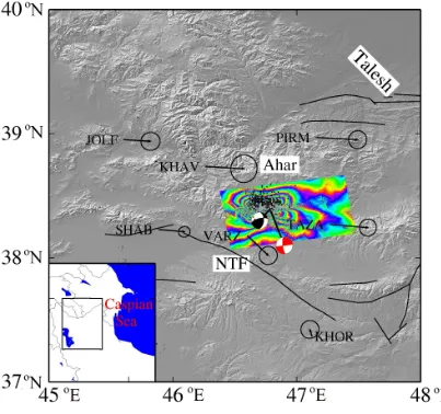
Figure 2.1 The location of August 11, 2012 Ahar earthquakes and the corresponding focal mechanisms from Global CMT solutions. The aftershocks are recorded by IIEES

(http://www.iiees.ac.ir/English/). The vectors are the GPS velocities with respect to the

Central Iran block (Masson et al. 2007). NTF represents the North Tabriz Fault. The inset

shows the location of our study area within the northwest Iran. ...36

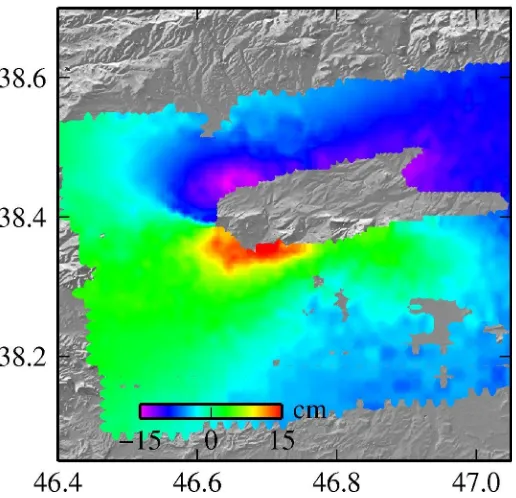
Figure 2.2 Observed DInSAR deformation without orbital errors removed ...38

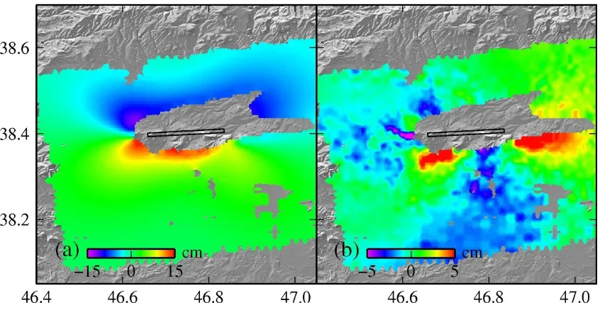
Figure 2.3 (a) Modeled displacement and (b) residual displacement from the GA solution for a single fault with a uniform-slip model. The surface expression of the modeled dislocations

is shown by a black rectangle. ...40

Figure 2.4 (a) Moment magnitude versus smoothing factor and (b) model roughness versus model residuals. The black square mark the location of the optimum smoothing factor and

the red squares mark two examples of extreme smoothing factors considered for comparison

...41

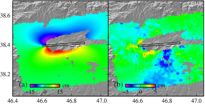
Figure 2.5 (a) Modeled displacement and (b) residual displacement on a single fault using a distributed-slip model (smoothing factor of 0.38). The surface expression of the modeled

dislocations is shown by the black rectangle. ...44

Figure 2.6 (a) Oblique slip, (b) strike slip and (c) dip slip on a single fault using a distributed slip model and smoothing factor of 0.38. The surface expression of the fault is shown in

Figure 2.5. ...45

Figure 2.7 (a) Modeled displacement and (b) residual displacement on a single fault using a distributed-slip model and a smoothing factor of 0.1. The surface expression of the modeled

dislocations is shown by a black rectangle. ...46

Figure 2.8 (a) Oblique slip, (b) strike slip and (c) dip slip on a single fault using a distributed slip model and a smoothing factor of 0.1. The surface expression of the fault is shown in

Figure 2.7. ...47

Figure 2.9 (a) Modeled displacement and the (b) residual displacement on a single fault using a distributed-slip model and a smoothing factor of 0.6. The surface expression of the

(14)

xiii

Figure 2.10 (a) Oblique slip, (b) strike slip and (c) dip slip on a single fault using a distributed slip model and a smoothing factor of 0.38. The surface expression of the fault is

shown in Figure 2.9...49

Figure 2.11 (a) Modeled displacement and (b) residual displacement on two faultsand using a distributed-slip model and a smoothing factor of 0.38. The surface expression of the

modeled dislocations is shown by a black rectangle. ...52

Figure 2.12 (a) Modeled displacement and the (b) residual displacement on two faults and using a distributed-slip model and a smoothing factor of 0.38. The surface expression of the

modeled dislocations is shown by a black rectangle ...53

Figure 2.13 Slip distribution on two faults using a distributed slip model and a smoothing factor of 0.38, on the (a) primary fault and (b) secondary fault. The surface expression of the

fault is shown in Figure 2.11...54

Figure 2.14 Slip distribution on two faults using a distributed slip model and a smoothing factor of 0.38, on the (a) primary fault and (b) secondary fault. The surface expression of the

fault is shown in Figure 2.12...55

Figure 2.15 Coulomb stress at (a) zero depth, (b) 5 km depth, (c) 10 km depth and (d) 15 km depth. At the middle of the fault and toward the east there is a decrease in the Coulomb stress

(15)

xiv

Figure 3.1 RGB amplitude image of San Francisco city acquired from RADARSAT-2 satellite (R: HH channel, G: VV channel, B: VH channel). The black line delineates the

approximate trace of the Hayward fault. The red square shows the close up region used for

interferometric analysis. The black and white figure shows the two subregions used for

further analysis in Figures 3.3-3.4. White and gray colors represents urban the rural areas,

respectively. ...71

Figure 3.2 Mean coherence maps, (a) HH, (b) VV, (c) VH and (d) optimized images. Improvement of PolInSAR coherence (d) is clearly demonstrated with respect to single-pol

channels (a-c). ...73

Figure 3.3 (a-c) Histograms of the mean coherences for the HH and the optimized polarimetric channels associated with (a) the entire image, (b) rural and (c) urban subregions.

(d-f) PCs increment after application of PolInSAR for an arbitrary coherence threshold. Here,

the horizontal axis represents the coherence threshold and the vertical axis is the increase in

the number of PCs from HH channel to the optimized channel, associated with (d) the entire

image, (e) the rural subregion and (f) the urban subregion. Note that the percentage is with

respect to the entire image pixels. (g-i) histogram of angle for the newly selected PCs in the

optimized compared to HH channel (with coherence threshold of 0.3) for the (g) entire image

pixels, (h) rural and (i) urban subregions, respectively. ...76

Figure 3.4 (a-c) Relative mean coherence improvement (with respect to initial HH coherence) for individual interferograms of different spatial and temporal baseline, for (a) the

entire image, (b) rural subregion and (c) urban subregion. ...77

Figure 3.5 Example of an interfreogram formed between dates 2008/06/13-2011/03/18 for the close up region in Figure 3.1. (a-b) refer to the HH and optimized interferograms for

pixels marked as PCs in each channel. (c-d) refer to the HH and optimized interferograms for

pixels only marked as PCs in the optimized channel. Comparison of the interferograms

shows that the main features of interferograms are preserved after application of PolInSAR

technique. Comparing (c) and (d) shows that the quality of phase improves after application

(16)

xv

Figure 4.1 SRTM Topography for the San Francisco region with RADARSAT-2 trajectories. The blue and green boxes mark the footprint of ascending and descending tracks,

respectively. The red lines represent the faults in this region. ...88

Figure 4.2 Linear deformation map derived from SBAS technique by using single-channel HH dataset for the (a) descending (d) ascending tracks. Linear deformation map derived from

SBAS technique by using single-channel VV dataset for the (b) descending (e) ascending

tracks. Linear deformation map derived from SBAS technique by using the optimized

channel for the (c) descending (f) ascending tracks. Note that here the LOS shortening is

represented by positive and LOS lengthening is represented by negative values. The black

lines represent the faults in this region, as in Figure 4.1. The black squares in (c) and (f) mark

the reference region for calibration of DInSAR images in the descending and ascending

geometries, respectively. ...96

Figure 4.3 Location of profiles in the PolInSAR deformation map marked by red lines and the numbers associated with each. The deformation rate along these profiles is presented in

Figures 4.4-4.5. The black lines represent the faults in this region, as in Figure 4.1. The black

line parallel to the Hayward fault in the north (identified by the black arrow) represents the

location of a secondary fault that may experience creep events. ...98

Figure 4.4 Linear rate of deformation along profiles in Figure 4.3, derived from descending images. The horizontal axis represents distance from Hayward fault. The red line marks the

location of Hayward fault. The black line in profiles (1-4) might be another fault parallel to

the Hayward fault in the north (the location is shown in Figure 4.3). ...99

Figure 4.5 Linear rate of deformation along profiles in Figure 4.3, derived from ascending images. The horizontal axis represents distance from Hayward fault. The red line marks the

location of Hayward fault. The black line in profiles (1-4) might be another fault parallel to

the Hayward fault in the north (the location is shown in Figure 4.3). ...100

Figure 4.6 Residual errors of linear deformation map derived from SBAS technique by using single-channel HH dataset for the (a) descending (d) ascending tracks. Residual errors of

linear deformation map derived from SBAS technique by using single-channel VV dataset

(17)

xvi

derived from SBAS technique by using the optimized channel for the (c) descending (f)

ascending tracks. Note that here the LOS shortening is represented by positive and LOS

lengthening is represented by negative values. The black lines represent the faults in this

region, as in Figure 4.1. The black squares in (c) and (f) mark the reference region for

calibration of DInSAR images in the descending and ascending geometries, respectively ..102

Figure 4.7 LOS linear displacement maps for the Berkeley landslides: Figures (a), (c) and (e) are the maps from ascending images derived from (a) the HH, (c) the VV and (e) the

PolInSAR optimized channel. Figures (b), (d) and (f) show the corresponding maps from

descending images derived from (b) the HH, (d) the VV and (f) the PolInSAR optimized

channel. Note that positive displacement represents motion toward the satellite. The black

and red polygons outline the location of moderately active and highly active slope

instabilities (USGS Earthquake Hazard Program 1999). The black dashed lines represent the

faults in this region, as in Figure 4.1. ...104

Figure 4.8 Optimized linear deformation maps for (a) ascending (b) descending tracks, overlaid on an aerial photography. The orange and red polygons outline the location of

moderately active and highly active slope instabilities (USGS Earthquake Hazard Program

1999). The black lines represent the faults in this region, as in Figure 4.1. ...106

Figure 4.9 Residual errors of linear deformation rate after application of the SBAS technique: (a), (c) and (e) are the maps from ascending images derived from (a) the HH, (c)

the VV and (e) the PolInSAR optimized channel. Figure 4.9 (b), (d) and (f) show the

corresponding maps from descending images derived from (b) the HH, (d) the VV and (f) the

PolInSAR optimized channel. The black and red polygons outline the location of moderately

active and highly active slope instabilities (USGS Earthquake Hazard Program 1999). The

(18)

Chapter 1

1

General Introduction

1.1.Introduction

Differential Interferometric Synthetic Aperture Radar (DInSAR) is a remote sensing

tool for measuring ground surface deformation induced by natural or man-made

processes. The interferometric approach is based on the phase comparison of synthetic

aperture radar (SAR) images gathered, via satellite, at different times with slightly

different looking angles (Massonnet & Feigl 1998; Bamler & Hartl 1998). DInSAR has

the advantage of mapping an area of hundreds of square kilometers with high spatial and

temporal resolution. This technique has additional advantage of mapping in all-weather

conditions. The deformation at the ground surface may reflect the distribution of stress in

the subsurface and provide more detail on both the past and future behavior of the surface

deformation and its associated causes. In this regard, inverse modeling is required to

obtain knowledge about subsurface processes from these surface measurements.

DInSAR has been used for monitoring volcano dynamics (Massonnet et al. 1995;

Manconi et al. 2010), coseismic displacements (Massonnet et al. 1993; González et al.

2013), subsidence due to exploitation of ground-water and oil/gas (Amelung et al. 1999;

Tiampo et al. 2012) and mining subsidence (Carnec & Delacourt 2000). Recently this

technique also has been used for the monitoring of deformation associated with carbon

sequestration and the melting of permafrost (Vasco et al. 2008; Short et al. 2012).

Multi-baseline DInSAR techniques have also been developed which are able to measure surface

deformation with milometer accuracy by using a larger number of SAR images (Sandwell

& Price 1998; Bernardino et al. 2002; Feretti et al. 2001; Hooper et al. 2007; Samsonov

& d’Oreye 2012).

The Ahar double earthquakes (Mw=6.4 and 6.2) struck northwest Iran on August 11,

2012. The earthquakes are located 50 km north from the largest and the most hazardous

(19)

order to map the co-seismic deformation using RADARSAT-2 SAR images. Moreover, I

applied inversion schemes to find the ruptured fault geometry and solve for its distributed

slip. Modeling of the surface deformation not only shows that the two events occurred on

one fault plane, it also provided important insights into the pattern of stress accumulation

and release in this region.

One of the drawbacks of DInSAR is that the radar signal decorrelates in the presence

of volume scattering such as vegetation cover and causes degradation of the

interferometric phase. This was a limitation on the study in Ahar, above. New radar

satellites have the capability of performing measurement in multi-polarizations, providing

more observations of the ground surface. In this work I implement Polarimetric SAR

Interferometry (PolInSAR), a technique for integrating polarimetry and interferometry in

order to increase the precision of DInSAR measurements. In addition, I apply this

technique to measure creep rate on Hayward fault, CA. This analysis demonstrates the

efficiency of this technique for providing a more precise interferometric phase

measurement.

In the following sections I will describe fully the basics of SAR, DInSAR and

Advanced DInSAR and PolInSAR techniques.

1.2.Synthetic Aperture Radar (SAR)

Synthetic Aperture Radar (SAR) is an imaging radar system onboard a moving

platform. In this system, electromagnetic waves are transmitted and the backscattered

echoes are collected. Due to the platform movement, each reception corresponds to

different positions in a SAR scene and each single pixel is assigned an azimuth and range

coordinate. The azimuth is the direction of platform movement and the range direction is

the Line-of-Sight (LOS) direction, the distance from the moving platform to the ground.

Figure 1.1 demonstrates that the 3-dimensional objects are projected to a 2-dimensional

(20)

and hyperbola. The circles are the lines of equal-distance (range) and the hyperbola are

the lines of equal-doppler (azimuth).

Figure 1.1. SAR image geometry and the location of pixels in range and azimuth direction (Massonnet & Feigl 1998).

A SAR image is a complex valued matrix, including amplitude and phase. Figure 1.2

is an example of a SAR amplitude image. The areas with higher reflectivity are brighter

in this image. However, a SAR phase image looks like a random noise image with values

ranging between 0-360 degrees. Each SAR image pixel represents the coherent sum of

(21)

Figure 1.2. An example of SAR amplitude image of an area in Mojave Desert, CA (Bamler & Hartl 1998)

Space-borne SAR systems operate with different radar wavelengths. The advantages

and disadvantages of choosing different wavelengths for interferometric applications will

be discussed in section 1.7. Table 1.1 lists space-borne SAR systems with the

corresponding imaging characteristics. SAR systems also operate in a variety of imaging

modes. This is done by altering the SAR antenna radiation pattern. These imaging modes

are: Stripmap, ScanSAR and Spotlight (Figure 1.3). For the Stripmap mode, the antenna

illuminates one swath and creates one single strip of radar data (Moreira et al. 2013). For

the ScanSAR mode the antenna illuminates different swaths with a shorter illumination

time which degrades the azimuth resolution (Ahmed et al. 1990; Bamler & Eineder

1996). The Spotlight mode is designed so that the antenna is steered illuminating a

(22)

Figure 1.3. Different imaging modes: (a) Stripmap, (b) ScanSAR and (c) Spotlight (Moreira et al. 2013).

1.3.SAR Geometry

In radar system, the slant-range resolution (dr) is dependent on the system bandwidth

and is derived by (1.1)

(1.1)

where c0 is the speed of light and B is the system bandwidth (Elachi 1987).

Older radar systems had the drawback of lower resolution in the azimuth direction.

This limitation has been overcome by the use of coherent radar and image processing

techniques (Wiley 1985), leading to an improvement of the azimuth resolution. The

resulting azimuth resolution ( ) is independent of the range distance and is equal to half

the azimuth antenna length () (Elachi 1987),

(1.2)

Raw radar images require initial processing in order to transform them into a

single-look (SLC) image, as shown in Figure 1.1. This includes filtering at both the range and

azimuth directions named as range compression and azimuth compression (Cumming &

Wong 2005). As the radar travels along the flight track, the transmitted pulses are linear

(23)

data in order to compress all the energy distributed over the chirp duration into as narrow

as a possible time window (Moreira et al. 2013). In this process each range line is

multiplied in the frequency domain by the complex conjugate of the spectrum of the

transmitted chirp. Figure 1.4 demonstrates the range and azimuth compression applied to

a raw radar data.

Because of the platform motion, the signal in the azimuth direction is modulated by

the doppler frequency. The azimuth focusing can be achieved by correlating the azimuth

line with a reference function in the frequency domain (Moreira et al. 2013). This will

give a focused SAR image in both the range and azimuth directions.

Figure 1.4. Summary of SAR processing steps where the range and azimuth compressed data result from a convolution of the raw data with the reference

(24)

1.4.SAR Radiometric Correction

The magnitude of the SAR image is not uniform over the entire image and is affected

by different factors, such as the pattern of the antenna diagram, the longer traveling path

of a wave in the far range compared to near range, etc. (Elachi 1987). In order to

compensate for these effects a radiometric calibration is needed to derive the radar cross

section normalized to the area. A calibrated SAR can be either in the 0 or in the γ0 form.

In the case the SAR image intensity corresponds to the backscattering coefficient

normalized to the horizontal ground surface. In the case of the SAR image intensity

corresponds to the normalized backscattering coefficient in the range direction (Freeman

1992).

1.5. SAR Image Statistics

One characteristic of SAR images is the speckle, which is caused by the presence of

many independent scatterers within one resolution cell (Goodman 1976). The coherent

sum of their amplitudes and phases results in strong fluctuations of the backscattering

from one pixel to the other. The intensity and the phase of SAR image pixels are not

deterministic, because of the presence of speckle noise, and follow an exponential and

uniform distribution, respectively (Oliver & Quegan 2004). The total complex reflectivity

() for each resolution cell is given by

′ ∑ ′

exp

. !" #$%_&′ , (1.3)

where , and r is the radar cross section, phase and range distance for each

individual scatterer. j is the number of the scatterer and (′_{is the wave number.}

In order to decrease the effect of speckle, a common technique such as multilooking is

applied. This technique is an averaging of the intensity image (Curlander & McDonough

(25)

SAR image resolution. However, by using this technique a better understanding of target

characteristics is achieved.

Table 1.1. Space-borne SAR system characteristics

Abbreviation Launch

Date

Band Repetitio

n Cycle

Maximum Resolution

(meters)

SEASAT 1978 L 3 25

ERS-1 1991 C 3, 35, 168 30

ERS-2 1995 C 35 30

JERS-1 1992 L 44 18

Radarsat-1 1995 C 24 10

SIR-C 1994 X, C, L Variable 18

ENVISAT 2002 C 35 30

SRTM 2000 C, X 35 12

ALOS 2006 L 46 10

TerraSAR-X 2007 X 11 1

TanDEM-X 2010 X 11 1

Radarsat-2 2007 C 24 1

COSMO –SkyMed-1/4 2007 X 16 1

RISAT-1 2012 C 25 3

HJ-1C 2012 S 4 5

1.6. Differential Interferometric Synthetic Aperture Radar (DInSAR)

An interferogram is formed by pixel-wise multiplication of the complex backscattering

signals, V, of two SAR images (Bamler & Hartl 1998),

)*, " )+*, "),*, " |)+*, "||)*, "| !"./0*, "1 (1.4)

where * denotes the complex conjugate, 0 0# 0₊ is the interferometric phase, and

(26)

azimuth coordinates. Figure 1.5 displays an example of an interferogram from Bam

earthquake, where each cycle represents 28 mm of displacement in LOS direction.

Figure 1.5. Satellite interferogram of Bam earthquake (Mw= 6.5, 26 December 2003). Each fringe represents 28 mm of displacement in the LOS satellite direction

for C-band which 56 mm (Motagh et al. 2006).

The interferometric phase results from the following contributions determining

differences in the propagation path length between the two images:

0 023 043 053 063 789! (1.5)

where 0₂ and 0₄ are the phase differences associated with the flat earth and

topography (Massonnet & Feigl 1998). Flat earth component is the effect of a distance

(27)

is the effect of elevation, which depending on the perpendicular baseline (:_;) produces

additional phase component. The perpendicular baseline is the distance between two

antenna positions, perpendicular to the LOS direction.

0₆ is the phase difference due to changes in atmospheric propagation. The atmospheric phase variation is dominated by water vapour (Hanssen 2001). It is not

possible to correct for atmospheric effects in a single interferogram without information

on the state of the atmosphere from other data sources. The atmospheric delay gradient

can be in the order of up to 1cm/km or more (Hanssen 2001). 0₅ is the phase difference

due to displacement of the observed surface element in LOS.

We can expand equation (1.5) to (1.6):

0 $%_<_′:_;3_λ′_=5;>$% _′:_;?@ 3$%_<_′ 3 0₆3 789! (1.6)

?@ is the surface elevation and A′is the radar look angle, is the surface displacement, and λ′ and are the radar wavelength and satellite-ground distance,

respectively.

Elimination of all the phase components (flat earth, topographic phase), will give the

phase difference due to displacement. The topographic phase is eliminated using an

external digital elevation model (DEM). Any inaccuracy in the external DEM translates

into a phase error in the final interferograms. The displacement and its phase are related

using the following formula:

0 0# 0+ $_λ′π# + (1.7)

Subscripts 1 and 2 refer to two SAR images acquired at two different times.

Accordingly, one complete phase cycle (2π) corresponds to half a wavelength (λ′ of

displacement; e.g. if the radar system has a wavelength of 6 cm, one fringe is equivalent

to 3 cm of deformation in LOS direction. Before conversion of phase to displacement, it

should be noted that the resolved phase difference is a wrapped value and a phase

(28)

number between [0,2C]. The phase unwrapping algorithm starts from a random point in

the image and integrates the phase values along a path to retrieve the absolute phase

corresponding to each image pixel. Theoretically, phase unwrapping is not affected by

the choice of its path. But this condition does not hold everywhere due to decorrelation

noise or steep topography (Bamler & Hartl 1998).

The processing of DInSAR data starts by the selection of two images which have a

reasonable spatial and temporal baseline. The maximum spatial baseline is on the order of

several hundred meters. The correlation between the two complex SAR images decreases

with increasing spatial baseline until it completely vanishes. This baseline is known as

the critical baseline for flat surfaces (Rodriguez & Martin 1992). However, the maximum

temporal baseline is a factor of any change in the ground cell, e.g. land cover change, soil

moisture change. The temporal baseline varies from several days to few years. Figure 1.6

demonstrates the different steps of interferometric processing.

The first step of processing is the coregistration of the second image (slave) with

respect to the first image (master). After the coregistration, the interferogram is made by

subtracting the phase value of the two images using equation (1.5) (Figure 1.6 (a)). Later,

different interferometric contributions are subtracted including the flat earth and

topographic effects. The resulting image is the interferogram which shows the phase

difference due to displacement, assuming that the atmospheric noise is negligible (Figure

1.6 (b)). The next step is the phase unwrapping and conversion of the phase to

displacement using equation (1.7) (Figure 1.6 (c)).

DInSAR is sensitive to only the component of the velocity vector in the LOS (in slant

range) and not to the component of motion along track. The LOS projection of

deformation can be obtained as the scalar product of displacement (d) and the DInSAR

sensitivity vector (u):

DEF . G H

I

;=J

KI;5J

L HGG;=JI

GKI;5J

L Hsin A . P89sin A . 97

(29)

where A is the look angle and is the satellite heading angle. It is possible to retrieve

more information about the ground movement by analyzing images from different

ascending and descending geometries. In that case there will be more observations (LOS)

available in order to invert for the three-dimensional components of surface

displacement. When the incidenet angle is higher, the sensitivity to the vertical motion is

decreased.

Figure 1.6 (a) Initial interferograms of Bam earthquake (Mw= 6.5, 26 December 2003) (b) the final interferogram after removal of orbital and topographic contribution and (c) the final displacement map showing the amount of deformation

(Motagh et al. 2006).

1.7. Coherency

The interferometric coherence γcan be computed as (Bamler & Hartl 1998),

Q RSTUTV,W

XRS|TU|VWRS|TV|VW 0 Z |Q| Z 1 (1.9)

where E{ . } represents the expectation value. The module of the interferometric

coherence |γ|, called the coherence (Figure 1.7), is a measure of the phase noise of the

(30)

The relationship between the coherence and the phase variance was explored by many

authors (Zebker & Villasenor 1992; Joughin et al. 1994; Rodriguez & Martin 1992). This

relationship was expressed by Zebker & Villasenor (1992) as

\ +

]^ +_`V

`V (1.10)

where N and M are the number of looks in range and azimuth direction. In a practical

sense, one can form a coherence map from the data and use equation (1.10) to quantify

the phase and deformation errors.

Each pixel in a SAR image is composed of several scatterers with different reflectivity

and the differential sensor-target path. If these values do not change in the time span

between successive radar acquisitions, they are cancelled out from the interferometric

phase. This is the basic assumption for carrying out interferometric measurements and

corresponds to full coherence. The interferometric coherence can be formulated as a

composition of the following contributions (Rodriguez & Martin 1992)

Q Q4=I=. QJI=6. QI64=. Q45 (1.11)

where Q_4=I= refers to the phase errors introduced by SAR processing; these errors

are usually small and Q_4=I= is close to one. Q_JI=6 is dependent on the

signal-to-noise ratio of the SAR system. Q₄₅ expresses the decorrelation due to changes

caused by different reflectivity at the two ends of the baseline (Zebker & Villasenor

1992). In the case of pure surface scattering, the decorrelation can be eliminated by

filtering of the range spectra (Gatelli et al. 1994). In this regard, optimum slope-adaptive

spectral shift filtering can improve further interferogram quality (Bamler & Davidson

1997). Spectral shift increases with terrain slope to the point where it equals the range

system bandwidth. Beyond the look angle spectral shift is negative due to layover (Gatelli

et al. 1994). Q_I64= represents temporal decorrelation caused by changes in the

distribution of scatterers within the resolution cell occurring during the time interval

(31)

The main limitations for the application of DInSAR over long time intervals result

from temporal decorrelation. In densely vegetated areas, such as forests and agricultural

lands, the signal usually decorrelates within days. On the other hand, over areas with low

vegetation or bare surfaces the signal may remain coherent over several years. The loss

of coherence due to vegetation is most significant for short wavelengths (X and C band).

Conversely, the longer wavelengths (L band) can penetrate deep into vegetation and

result in less volume decorrelation.

Figure 1.7. Coherence image of a RADARSAT-2 interferogram from the Ahar 2012 earthquakes.

1.8. Advanced DInSAR Techniques

There exist a number of advanced DInSAR methods which are widely used to measure

deformations of Earth’s surface with higher accuracy than conventional DInSAR

(Sandwell & Price 1998; Bernardino et al. 2002; Feretti et al. 2001; Hooper at al. 2007).

One of the examples of these techniques is stacking (Sandwell & Price 1998), in which

(32)

Another widely used technique is the Small Baseline (SBAS) method (Bernardino at

al. 2002; Samsonov et al. 2011). This methodology selects interferograms with small

spatial and temporal baselines, assuming a minimum effect of decorrelation noise for

these interferograms and a constant displacement velocity between subsequent

acquisition times. Using Singular Value Decomposition (SVD), this technique solves for

the deformation rate between subsequent radar images. Additionally, the residual

topographic phase also is formulated as a function of perpendicular baseline and resolved

in this technique. Later, the atmospheric phase is removed by applying a high pass

filtering in time and low pass filtering in space.

Permanent Scatterer (PS) and Coherent Pixel method (CPM) (Feretti et al. 2001;

Hooper at al. 2007, 2008; Blanco-Sánchez et al. 2008) are also techniques to improve the

quality of the interferograms. The idea is to select radar phase stable points within a radar

scene, assuming that the effect of decorrelation noise is minimum for these objects.

These points, called Pixel Candidates (PC), usually correspond to buildings, metallic

objects, exposed rocks and other stable, reflective surfaces that exhibit a constant radar

signature over time. After interferogram generation, the phase of the PCs can be

decomposed into several contributions including displacement phase, atmospheric phase

and residual topographic phase. The least squares method is applied in order to retrieve

the absolute phase value corresponding to each radar scene and in the meantime solves

for other phase components.

Multibaseline DInSAR techniqueas need a large number of coherent pixels to work

properly (Feretti et al. 2001). The quality criteria for selecting these coherent targets

(Pixel Candidate (PC)) are the average coherence for the full set of interferograms. In this

technique, the interferograms are formed and a thresholding is applied over the mean

coherence to separate the pixels with the higher coherence value (Blanco-Sánchez et al.

2008). The second criterion is based on the amplitude dispersion index (Feretti et al.

2001). The amplitude dispersion index is computed for the whole stack of single-look

complex images from the following formula:

(33)

where h is the mean and is the standard deviation of a pixel in different radar

scenes. This value provides an indication about the phase stability of the corresponding

pixel.

In the next sections, I will explain how the use of polarimetric information will

increase the number of PCs for Advanced DInSAR. An example of this technique is the

Polarization Phase Difference (PPD) method (Samsonov & Tiampo 2011) which selects

pixels that demonstrate either even or odd bounce scattering properties, using a number

of polarimetric images.

1.9. SAR Polarimetry

A radar polarimetric system measures the polarization state of a wave backscattered by

the media. The measured polarimetric signal depends on the type of scattering

mechanisms (SM), which is a representation for polarization states in the transmitted or

backscattered wave.

SAR polarimetry is a technique used for acquiring physical information from different

land covers. Previous studies have used polarimetric scattering models to provide

information about physical ground parameters such as soil moisture and surface

roughness (Hajnsek et al. 2003; Hajnsek et al. 2007). Moreover, the temporal evolution

of these observables provides information on the temporal changes of these parameters

(Mattia et al. 2003). Unsupervised classification methods of polarimetric data identify

different scatterer characteristics and target types (McNairn & Brisco 2004).

1.10.Principles of SAR polarimetry

In satellite radar polarimetry we analyze the shape of the transmitted and received

polarization ellipse, as shown in Figure 1.8. This figure shows the spatial helix resulting

from a combination of horizontal (H, in green) and vertical (V, in blue) transmitted

components. When a radar wave is transmitted in a horizontal polarization and received

(34)

radar wave is transmitted with a vertical polarization and received with horizontal or

vertical polarizations, it is called VH or VV channels.

Figure 1.8. The polarization ellipse decomposed into orthogonal components x (horizontal H) and y (vertical V)

(http://www.nrcan.gc.ca/earth-sciences/geography-boundary/remote-sensing/radar/1968).

A radar wave is described using a pair of complex numbers, !_i and !_j as shown in the

following equation, in any polarimetric basis, corresponding to the horizontal and vertical

component of the wave.

!i3 !j k l m_!!i_jn (1.13)

Fully polarimetric SAR (Pol-SAR) sensors acquire images in various polarimetric

channels and ultimately can measure the 2×2 scattering matrix, S, corresponding to the

media, as

l Iop′q = rs5

tt _s 5tT

s5Tt s5TTu l

(35)

l_{is the scattered wave and}_l_{is the transmitted wave. Here}_r_{is the distance from the}

satellite to the ground point and (′ is the wave number. The scattering matrix is

independent of the transmitted polarimetric basis; it is a function of shape, orientation and

dielectric properties of the scatterers. Under the reciprocity theorem, the off-diagonal

elements are equal and s_tT s_Tt. The scattering matrix is expressed as a scattering

vector (k) using the Pauli basis as (Cloude & Papathanassiou 1987)

(5 _√+ ws5tt3 s5TT, s5tt# s5TT, 2s5tTxy (1.15)

SAR polarimetry has the capability of discriminating different types of scattering

mechanisms within a resolution cell. The radar targets are categorized as deterministic

and distributed targets. Deterministic targets are the point-wise scatterers and distributed

scatterers are those composed of a large number of randomly distributed deterministic

scatterers. The scattering matrix is able to completely describe deterministic scatterers.

However, for the distributed targets, a second-order statistics is required, such as

coherency [T] matrix (equation 1.16).

z {((,y_| _(1.16)

where *T represents conjugate transpose operator and ⟨⟩ is the multilooking factor.

Using a multilooking approach the effect of the single scatterers is decreased and the

mean value is achieved for a group of pixels.

1.11.Polarimetric SAR Interferometry (PolInSAR)

In Polarimetric SAR Interferometry (PolInSAR), Interferometric SAR (InSAR) and

polarimetric techniques are coherently combined to provide improved sensitivity to the

vertical distribution of scattering mechanisms (Cloude & Papathanassiou 1998). Using

the PolInSAR technique, it is possible to extract scatterers at different heights for a given

(36)

Coherence is the main observable of PolInSAR. Coherence optimization is a technique

which attempts to find the best polarization base transformation corresponding to the

scatterer with the maximum coherence (Neumann at al. 2008). When this transformation

is applied to fully polarized satellite data, it will result in isolating the most dominant

scattering mechanism of the corresponding pixel (Papathanassiou & Cloude 1998; Colin

et al. 2006). Dominant scattering mechanisms provide each resolution cell with the

highest coherence value.

The advantage of this technique is to increase the component corresponding to the

most stable target, which is done by eigenvalue decomposition of the coherency matrices

in an optimization solution. The correspondence between the backscattered power and

stable radar targets is explained better in Section 1.8, where the amplitude dispersion

index is used as a measure to separate the stable radar targets. These points have less

spatial and temporal decorrelation noise.

In the previous studies, PolInSAR coherence optimization was employed to increase

the number of interferometric coherent pixels for DInSAR studies. This is achieved by

finding the optimum scattering mechanisms in a resolution cell through analysis of

average target’s coherency matrix (Navarro-Sanchez et al. 2010). As we use a number of

SAR images for advanced DInSAR analysis, a multibaseline approach must be

implemented. A multibaseline approach will guarantee that the scattering mechanism of a

SAR image will remain the same between all the interferograms. Otherwise, each SAR

image will have a different scattering center corresponding to each interferograms and a

noise component will be added to the differential phase. The noise corresponds to the

height difference between different phase centers.

There are two approaches to solve the multibaseline coherence optimization problem;

Multi-Baseline Equal Scattering Mechanism (MB-ESM) and Multi-Baseline Multiple

Scattering Mechanism (MB-MSM). In the case of MB-ESM as proposed by (Neumann et

al. 2008), the scattering mechanisms of the images remain the same among all the

baselines (ω ω. However, this condition is not met using MB-MSM technique

(37)

correlates best to all others. MB-MSM technique can introduce an additional

interferometric phase of the DInSAR method. While in reality some physical effects (e.g.

change in soil moisture content, incident angle and atmospheric conditions) will modify

the scattering mechanisms between acquisitions, leading to temporal decorrelation, the

change of scattering mechanism between acquisitions might compensate for the temporal

decorrelation in areas of less noise. If there is no meaningful change of the scattering

mechanism, the MB-MSM technique may add a component to the interferometric phase.

This additional phase component (noise) corresponds to the difference of the phase

centers from assumption of the two different scattering mechanisms at two ends of the

baseline.

Accordingly, in previous research, the ESM has been applied instead of the

MB-MSM technique (Navarro-Sanchez et al. 2010), even though in some cases, the choice of

MB-MSM may provide better resolution of the interferometric phase. The technique to

solve the coherence optimization problem will be presented in the next section 1.12.

1.12. Methodology

Coherence optimization of polarimetric images is applied to reduce the interferometric

phase noise. As mentioned in section 1.7, different components of decorrelation degrade

the interferometric phase. PolInSAR coherence optimization is able to reduce the

component of volume scattering by selection of an optimum polarimetric channel. In this

technique the scattering mechanism corresponding to the highest coherence is retrieved,

which insures less interferometric noise. In multibaseline interferometry, as explained

before, mean coherence is an estimation of phase noise. Using the coherence optimization

approach, the mean coherence over a stack of interferograms will increase. Accordingly,

it will result in a higher number of coherent targets.

Here, I will explain in detail the processing steps employed in the multibaseline

(38)

1.12.1.Co-registration

The co-registration procedure aligns SAR images into the master image geometry. In

the first step, the satellite orbits are used for initial image co-registration. A more accurate

co-registration is performed by cross-correlation of the intensity images. The peak of the

correlation function will resolve the range and azimuth offsets. A number of windows are

distributed over the image and offset values for each patch are generated. A least squares

polynomial fit is used in order to find the model of the pixel offsets for the entire slave

image. Later, resampling of the slave image is performed using a complex sinc

interpolator.

The processing starts with the collection of SAR images at different dates (i=1 to

N+1). Each SAR image has three different polarimetric channels, assuming that the

reciprocity theorem holds. The co-registration is performed in two steps. The first step is

to co-register three different channels of the master image. In the next step, the remainder

of the SAR images are co-registered with the master image of the corresponding

polarimetric channel (HH,VV,VH).

1.12.2.Baseline Estimation

The next step of the analysis is to form all the possible pairs between the SAR images.

The condition to form an interferogram between two SAR images is dependent on the

spatial and temporal baseline. Where these baselines exceed the critical limit, the

displacement will be contaminated by decorrelation noise and the interferometric phase

will not be reliable. The maximum temporal baseline is dependent on the atmospheric

condition, land-cover change, soil moisture change, vegetation groth, etc. and can vary

between a few months to several years. The maximum spatial baseline is a function of the

look angle and the wavelength and distance from the satellite to the ground.

1.12.3.Coherence Optimization

After the above steps are complete, I perform coherence optimization of the fully

(39)

optimization is applied in order to constrain the scattering mechanisms to be equal at both

ends of the baseline. The optimization solves for the highest mean coherence among all

the interferograms, as:

b " ∑ ∑ |Q 5 5| (1.17)

where ₊ _;

Q5 is the interferometric coherence between images i and j corresponding to the scattering mechanism . In the following equation, equality is achieved when the phase

shift (A₅) is equal to the optimum coherence phase values.

b " ∑ ∑5+; ;+Q5!_5>o Z b " ∑ ∑5+; ;+|Q5| (1.18)

Accordingly, an iterative numerical approach as presented below is applied in order to

introduce an optimal phase shift:

∑ ∑ ;₅ ; ₅!_5>o (1.19)

5 zI_+/5zI_+/ (1.20)

zI +_;∑ z;5+ 55 (1.21)

Xy

_Xy (1.22)

A5 arg 5 (1.23)

In these equations, by iteratively changingA₅, we get a better estimation of the optimal

phase value. In accordance with Neumann et al., 2008, the optimization is performed as

follows:

1) Initialization; A₅ arg.c P!₅1 ; 0.

2) Derive H and w, and solve for the eigenvalue and the corresponding phase shift.

3) Improve the estimation of A₅.

4) The process stops if the phase shift is below a certain threshold.

5) Use w in order to solve for the .

(40)

pixels is selected in order to calculate the coherency matrices and the corresponding

scattering mechanisms. When these mechanisms are found, they are converted from the

linear basis (H,V) to the optimal basis. As a result, for each SAR image, instead of having

three channels of (HH,VV,VH) data, one optimized channel is resolved.

1.12.4.Interferogram Generation

Before interferograms generation, common-band range and azimuth filtering is

performed on the SAR images. The two SAR images are acquired from slightly different

look angles and the slant range spectra of two images may not overlap completely.

Moreover, if the squint angle of the two SAR images is different, there is a difference in

the azimuth spectra. These effects will cause decorrelation and the filtering is applied

before interferograms generation to remove the decorrelation effect at the price of

reduced resolution.

Differential interferogram generation is formed by calculating the phase difference of

two SAR images (1.4). The processing window size is consistent with the window size

used for the coherence optimization. The choice of a 5×10 pixel processing window is

made to ensure that enough independent scatterers occur in a given resolution cell and

produce an unbiased estimation of coherence (Touzi et al., 1999). For a smaller window

size the scatterers might not be independent from each other. Moreover, there is a

trade-off between the size of the processing window and spatial resolution. Selecting a small

averaging window ensures higher spatial resolution, but biases the coherence estimation

towards higher values.

Equations (1.5) and (1.6) are used to remove the topographic component and the flat

earth component. Later, I will explain the procedure to remove the residual orbital

components and the residual topographic components.

1.12.5.Phase Unwrapping

The next step in DInSAR analysis is to filter the interferograms to reduce the

interferometric phase noise. After the interferometric generation and filtering, the

(41)

Minimum Cost Flow (MCF) (Costantini & Rosen, 1999). The steps of the phase

unwrapping are as follows:

1) A set of coherent points above a certain threshold are selected and connected by a

delaunay triangle network.

2) The minimum cost flow algorithm is employed in order to connect the residues. A

residue is a point in the interferogram where the sum of the phase differences

between pixels around a closed path is not 0.

3) Unwrapped phases are computed by integration.

The application of PolInSAR coherence optimization will result in different scattering

mechanism for the neighboring pixels. However, the effect of polarimetric change from

one pixel to another will not significantly change the performance of the phase

unwrapping. Assuming that the relative position of the scatterers in a resolution cell does

not change significantly, phase unwrapping can be applied to the neighboring pixels from

different scattering mechanisms. Accordingly, the coherence optimization solves for the

optimized scattering type, which is more stable in time, in order to give better

deformation estimation. In the remainder of this research, the mean quality criterion is

used for separation of the most stable targets. A coherence threshold of 0.3 is employed to

separate the group of coherent and non-coherent pixels as explained in Section 1.8.

1.12.6.Residual Orbital Error Correction

In cases where there is an inaccuracy in the position of the satellite, there is a

systematic error which remains after removal of the flat earth component. The systematic

error is a long wavelength fringe pattern across a single interferograms. Removal of

residual orbits is performed by fitting a plane to the phase measurements. The

coefficients of a bilinear plane are derived using a regression technique, and the synthetic

(42)

1.12.7.Multibaseline Analysis

The multibaseline DInSAR approach used in this thesis is the Small BASeline (SBAS)

technique developed by Berardino (2002). In this technique only interferograms of small

temporal baseline are selected in order to reduce the decorrelation noise. However, by

choosing these interferograms, there is a possibility that no common image exists

between some interferograms. In this problem, in order to avoid inversion singularity, the

Singular Value Decomposition (SVD) technique is employed, as explained below. The

technique solves for the residual topographic contribution and employs a Fast Fourier

Transform approach to reduce atmospheric artifacts. Since atmospheric errors are

long-wavelength features in the interferograms, we employ a low-pass filtering technique to

remove these signals. The SBAS technique first performs phase unwrapping to solve for

the absolute phase value. Then the unwrapped interferograms undergo a system of

equations to retrieve deformation time series using the following procedure.

We assume that there are N+1 images acquired at different times. The number of

possible interferograms with small spatial and temporal baseline can be calculated based

on the following:

]+

Z Z

]+

(1.24)

Accordingly, any phase difference between two SAR images, can be written as:

∆0 0pU# 0p $%_< .pU # p1 (1.25)

Where d is the deformation regarding the time t or t +1. Assuming that the deformation

at the first SAR image acquisition time is zero, the absolute phase at different SAR image

acquisition times is a vector of N components. We can formulate the above equations in

terms of surface velocity as:

∆0 $%_< c&+# c&. )pU,p (1.26)

The vector of unknown values is the velocity between two SAR image acquisitions,

assuming the deformation for the first SAR image acquisition is zero, as:

w)U, )V, … , )x (1.27)

(43)

∆0 w∆0U, ∆0V, … , ∆0x (1.28)

The matrix form of these set of equations is formulated as:

a ∆0 (1.29)

A is the matrix of coefficients, composed of differences in time between SAR images.

The solution to this system of equations depends on the number of interferograms and the

rank of matrix A. If the interferograms are such that there is a link between each SAR

image, then matrix A is not rank deficient and the problem can be solved by a least square

technique. Otherwise, A is decomposed as following

a s)y _(1.30)

U is an M×M orthogonal matrix, S is M×M diagonal matrix and V is orthogonal N×M

matrix. The solution is identified by minimum norm of the velocity (unknown) values.

Additional to the velocity vectors (v), it is possible adding additional terms in order to

remove the residual topographic errors.

wa xw x _∆0_(1.31)

w_<¡ $%_¢U£

¤¥¦§¨…

$% <¡_¤¥¦§¢£ ¨x

In order to simplify the inversion, we can reduce the deformation rates only to a linear

term. Accordingly, the problem is a linear regression to the observations, where we can

simultaneously solve for the residual topographic errors. For this regression problem we

derive the standard deviation of the observations from the model. In chapter 4, I will use

this standard deviation as a measure to compare the performance of PolInSAR technique

versus standard interferometry.

1.13.Purpose of study

The primary objective of my thesis is to develop tools aimed at increasing the

usefulness of DInSAR measurements in modeling and understanding of earth processes

by improving its accuracy and precision. This is achieved by incorporating fully

(44)

information with the DInSAR technique in Polarimetric SAR Interferometry (PolInSAR).

A secondary objective was achieved through the application of a standard DInSAR

analysis to the Ahar double earthquakes (August 11, 2012), in order to understand the

patterns of stress accumulation and release associated with the ruptured fault.

Unfortunately, fully polarimetric data was unavailable for this region, but this study has

important implications for future seismic hazard assessments because the event occurred

in the proximity North Tabriz Fault (NTF), the largest and the most hazardous strike-slip

structure in NW Iran. Understanding the Ahar fault structure and its pattern of stress

accumulation provides insights into its impact on the seismic activity of the regional

faults. The limitations of this study inherent in the higher decorrelation arising from the

standard InSAR method provide an important example of the necessity for employing

polarimetric data.

I pursued these goals through the following studies:

• Measuring co-seismic deformation of Ahar earthquake using standard

mode RADARSAT-2 interferograms. Advanced inversion methodologies were

implemented in order to model the ruptured fault plane.

• Developing a general framework to exploit newly available polarimetric

information of RADARSAT-2 in order to increase the number of coherent pixels

for DInSAR analysis and assessing the accuracy of their interferometric phases.

• Application of the PolInSAR coherence optimization technique to the

Hayward fault (San Francisco) in order to better assess the creep rate along this

fault; measuring the velocity of the landslides on Berkeley hills and comparison

of the deformation maps with the conventional DInSAR deformation.

1.14.Organization of work

This integrated thesis is presented in six chapters. The introductory chapter (Chapter 1)

(45)

the analysis of the Ahar double earthquakes derived from the standard DInSAR analysis.

Chapter 3 presents the results of the PolInSAR coherence optimization and shows the

improvements in terms of Pixel Candidates (PCs) and higher interferometric phase

precision. Chapter 4 presents a detailed application of the PolInSAR technique for the

Hayward fault and investigates the landslide motion in the Berkeley Hills. Finally,

Chapter 5 presents the concluding remarks and suggestions for future research.

1.15.References

Ahmed, S., Warren, H. R., Symonds, D. & Cox, R. P. 1990. The Radarsat system.

IEEE Trans. Geosci. Remote Sens. 28, 598-602

Amelung, F. et al. 1999. Sensing the ups and downs of Las Vegas: InSAR reveals

structural control of land subsidence and aquifer-system deformation. Geology, 27, 483-486

Bamler, R. & Davidson, G. W. 1997. Multiresolution signal representation for phase

unwrapping and interferometric SAR processing. Int. Geosci. Remote Sens. Symp.

(IGARSS), Singapore, 865-8

Bamler R. & Eineder, M. 1996. ScanSAR processing using standard high precision

SAR algorithms. IEEE Trans. Geosci. Remote Sens. 34, 212-18

Bamler, R & Hartl, P. 1998. Synthetic aperture radar Interferometry. Inverse Probl.

14, 1- 54

Berardino, P. et al. 2002. A New algorithm for surface deformation monitoring based

on small baseline differential SAR interferograms. IEEE Trans. Geosci. Remote Sens.,

40, 2375-2383

Blanco-Sánchez, P. et al. 2008. The Coherent Pixels Technique (CPT): and advanced

Application of Differential and Polarimetric Synthetic Aperture Radar (SAR) Interferometry for Studying Natural Hazards

Scholarship@Western

Scholarship@Western

Application of Differential and Polarimetric Synthetic Aperture

Application of Differential and Polarimetric Synthetic Aperture

Radar (SAR) Interferometry for Studying Natural Hazards

Radar (SAR) Interferometry for Studying Natural Hazards

Abstract

Keywords

Co-Authorship Statement

Acknowledgments

Table of Contents

List of Tables

List of Figures

Chapter 1

1

General Introduction