Resonances from lattice QCD

(1)

Resonances from lattice QCD

Raúl A.Briceño1,2,

1_{Thomas Jefferson National Accelerator Facility, 12000 Jefferson Avenue, Newport News, VA 23606, USA} 2_{Department of Physics, Old Dominion University, Norfolk, VA 23529, USA}

Abstract.The spectrum of hadron is mainly composed as shortly-lived states (resonance) that decay onto two or more hadrons. These resonances play an important role in a vari-ety of phenomenologically significant processes. In this talk, I give an overview on the present status of a rigorous program for studying of resonances and their properties using lattice QCD. I explain the formalism needed for extracting resonant amplitudes from the finite-volume spectra. From these one can extract the masses and widths of resonances. I present some recent examples that illustrate the power of these ideas. I then explain sim-ilar formalism that allows for the determination of resonant electroweak amplitudes from finite-volume matrix elements. I use the recent calculation of theπγ_→ _ππ_amplitude

as an example illustrating the power of this formalism. From such amplitudes one can determine transition form factors of resonances. I close by reviewing on-going efforts to

generalize these ideas to increasingly complex reactions and I then give a outlook of the field.

1 Introduction

Hadronic resonances are ubiquitous in nature, and as a result play an essential role in a variety of phenomenologically significant processes. One such example is the famous∆I = 1/2 rule in

K → ππweak decays. This empirical “rule” states that hadronic decay of the kaon to two pions is dominated by the process where the isospin of the final state is zero. The corresponding amplitude is approximately an order of magnitude larger than that when theππfinal state is projected onto an isotensor configuration. This somewhat surprising observation becomes quite natural when one remembers that the isoscalar channel contains theσresonance, which is nearly degenerate with the kaon, while the isotensor channel contains no resonances.

By now there is overwhelming evidence that without resonances most atomic nuclei would not be able to form. This is seen for example in the essential role played by resonances, in particular the σ, ρ,andω, in the construction of phenomenological potentials that accurately describe experimental data [1]. Another example is the well known Hoyle resonance, without which there would not be enough carbon, oxygen, nickel, etc. to support life as we know it [2].

(2)

energies. This is the motivation of a substantial experimental effort to precisely measure the basic

properties of resonances (mass, decay widths, couplings, etc.) and also explore the fringes of the hadronic spectrum, where these rules can be put to a test. Prominent examples include the searches for exotic in the GlueX and COMPASS experiments, tetraquark1_{and pentaquarks searches in Belle,}

BES and LHCb among other.

Given these and other experimental efforts, there is a strong demand for a parallel theoretical

program. Here I outline a theoretical effort to have a program that satisfies the following four criteria:

• confirmation of existence: there is a long list of states that are awaiting theoretical confirmation, plenty of examples can be found in the XYZ (see Ref. [5] for a recent review),

• predict existence: presently rigorous theoretical predictions of non-conventional hadrons are ab-sent,

• identify production/decay mechanism: in order to expedite and guide experimental searches, it

would be useful to have a theoretical determination of the prominent production/decay mechanism

including couplings to corresponding channel,

• structural information: there are a variety of properties that are experimentally inaccessible but are essential to gain insight into the true nature of a corresponding state, e.g., gluonic structure of hybrid mesons.

Resonances, by definition, lie above at least one open threshold. Most, in fact, lie above multiple open thresholds where two or more particles can go on-shell. In order to have a complete understand-ing of these resonances, one would need to have a QCD-based effort that is capable of dealing with

multichannel, multiparticle systems. This is undoubtably a challenging and daunting task, but thanks to lattice QCD this is not an insurmountable challenge.

Lattice QCD efforts have largely been focused in the extraction of the spectrum and properties

of QCD stable states. This is mainly due to the fact that these are the states that are most readily accessible using standard lattice QCD techniques. In fact, given the present framework of lattice QCD calculations and the nature of resonant states, it is not at all obvious that the latter can be accessed via lattice QCD. Nevertheless, there has been tremendous progress that has allowed for the exploration of resonant processes that were previously thought to be inaccessible via lattice QCD (for a recent review in the field see [6]).

Before explaining the challenges associated with study resonances on the lattice, it is necessary to begin by reviewing the definition of resonances as complex-valued poles in unphysical sheets of scattering amplitudes. I review the building principles of this in Sec.2. In Sec.3, I discuss the formalism for extracting two-body scattering amplitude from the finite-volume spectrum obtained from lattice QCD calculations, and I illustrate the power of these ideas in the light mesonic sector. In Sec.4.1, I discuss extension of these ideas to extract electroweak amplitudes, focusing my attention to 1→2 processes. I present a recent example in Sec.4.2using the formalism discussed. Lastly, in Sec.5I speculate what the future holds for study of resonances on the lattice.

2 Scattering theory and composite states

Here I review some of the basic principles in scattering theory that are relevant for the discussion that follows. In particular, we need a rigorous definition of resonances and a prescription to obtain their information using lattice QCD. As it turns out, we can only access their informations from

(3)

governing the fundamental theory of the strong interaction,quantum chromodynamics(QCD), at low energies. This is the motivation of a substantial experimental effort to precisely measure the basic

properties of resonances (mass, decay widths, couplings, etc.) and also explore the fringes of the hadronic spectrum, where these rules can be put to a test. Prominent examples include the searches for exotic in the GlueX and COMPASS experiments, tetraquark1_{and pentaquarks searches in Belle,}

BES and LHCb among other.

Given these and other experimental efforts, there is a strong demand for a parallel theoretical

program. Here I outline a theoretical effort to have a program that satisfies the following four criteria:

• confirmation of existence: there is a long list of states that are awaiting theoretical confirmation, plenty of examples can be found in the XYZ (see Ref. [5] for a recent review),

• predict existence: presently rigorous theoretical predictions of non-conventional hadrons are ab-sent,

• identify production/decay mechanism: in order to expedite and guide experimental searches, it

would be useful to have a theoretical determination of the prominent production/decay mechanism

including couplings to corresponding channel,

• structural information: there are a variety of properties that are experimentally inaccessible but are essential to gain insight into the true nature of a corresponding state, e.g., gluonic structure of hybrid mesons.

Resonances, by definition, lie above at least one open threshold. Most, in fact, lie above multiple open thresholds where two or more particles can go on-shell. In order to have a complete understand-ing of these resonances, one would need to have a QCD-based effort that is capable of dealing with

multichannel, multiparticle systems. This is undoubtably a challenging and daunting task, but thanks to lattice QCD this is not an insurmountable challenge.

Lattice QCD efforts have largely been focused in the extraction of the spectrum and properties

of QCD stable states. This is mainly due to the fact that these are the states that are most readily accessible using standard lattice QCD techniques. In fact, given the present framework of lattice QCD calculations and the nature of resonant states, it is not at all obvious that the latter can be accessed via lattice QCD. Nevertheless, there has been tremendous progress that has allowed for the exploration of resonant processes that were previously thought to be inaccessible via lattice QCD (for a recent review in the field see [6]).

Before explaining the challenges associated with study resonances on the lattice, it is necessary to begin by reviewing the definition of resonances as complex-valued poles in unphysical sheets of scattering amplitudes. I review the building principles of this in Sec.2. In Sec.3, I discuss the formalism for extracting two-body scattering amplitude from the finite-volume spectrum obtained from lattice QCD calculations, and I illustrate the power of these ideas in the light mesonic sector. In Sec.4.1, I discuss extension of these ideas to extract electroweak amplitudes, focusing my attention to 1→2 processes. I present a recent example in Sec.4.2using the formalism discussed. Lastly, in Sec.5I speculate what the future holds for study of resonances on the lattice.

2 Scattering theory and composite states

Here I review some of the basic principles in scattering theory that are relevant for the discussion that follows. In particular, we need a rigorous definition of resonances and a prescription to obtain their information using lattice QCD. As it turns out, we can only access their informations from

1_{For recent lattice QCD e}_ff_{orts in searches for tetraquarks see Refs. [}₃_,₄_].

scattering amplitude. For simplicity, I will focus my attention to scattering amplitudes where there are at most two hadrons in the initial or final states, but I will not restrict the number of two-particle channels that might be kinematically open.2

By definition, resonances are unstable under the strong interaction. In other words, they cannot be identified as asymptotic states. Because they commonly manifest themselves as dynamical en-hancements in cross sections, they have been qualitatively understood as “bumps in cross sections”. Although this serves as a rule of thumb, it is a terribly unsatisfying definition. Furthermore, it is not hard to find examples of resonances that do not appear as clear bumps in cross sections, e.g. theσ and theκ. Alternatively, one can rigorously define resonances as poles in scattering amplitudes in the complex plane of the Mandelstam variable s ≡ E2_.3 _{This definition holds for both bound states}

and resonances. Bound states are real-valued poles below the lowest threshold, while resonances are complex-valued poles and typically lie above the lowest threshold.4 _{The value of the pole location}

(sR) are related the resonance’s mass (mR) and width (ΓR),√sR=mR−₂iΓR.

At every threshold, the scattering amplitude has a square-root singularity. Let M;ab be the

partial wave component of the scattering amplitude for incominga and outgoingb channels. For example, in Sec.3.3we will discuss S-wave wave scattering amplitudes whereaandbcorrespond to ππandKKscattering states. Having this notation, one can explicitly see this singularity by evaluating the imaginary part of the inverse of the amplitude,

ImM−1 (s)

ab =−δab

1 16π

2q

a

√_s Θ(s−sa), (1)

wheresa =(Ethra .)2 is the value of theaththreshold, andqa ∼ √s−sais the cm relative momentum

and the source of the square root singularity. This in turns results in there being 2N_{Riemann sheets for}

Nopen channels. Causality prohibits complex-valued poles in the physical Riemann sheet, defined by Im[qa] > 0∀i. As a result, only real-valued poles can exist in this sheet, namely bound states.

Furthermore, this tells us that resonances can only correspond to complex poles on the unphysical sheets, where at least one relative momentum satisfies Im[qa]<0.

This definition does several things for us. First, it explains why some resonances manifest them-selves as bumps in cross sections. Second, it explains how one can (and perhaps “should”) think of the evolution of resonances and bound states with the quark masses. If we zoom in to a given pole in the scattering amplitude and we now consider that the amplitude itself depend on the values of the quark masses, which I denote amq, we find

M;ab(s;mq)∼ga(mq)gb(mq)

sR(mq)−s . (2)

As we dial the quark masses we expectsR(mq) andga(mq) to vary, but there is no reason as to why in

general they might go to zero or infinity. As a result, with the quark mass we might expect poles to move in the complex plane, even change sheets, and their coupling could very well vary, but we do not expect them to evaporate. This qualitatively explains why we observe some resonances becoming bound for heavier quark masses. This also tells us that we should probably think of resonances and bound states more generically as composite states that for some range of parameters might be accidentallybound or not.

2_{For a pedagogical introduction to scattering theory and the theory of composite states see [}₇_]. 3_E_{is the center of mass (cm) energy of the system, sometimes also labeled}_E

cm.

(4)

0 30 60 90 120 150

400 500 600 700 800 900 1000

(a) (b)

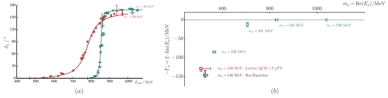
Figure 1. (a) Shown are theππisovector scattering phase shift from Refs. [8,9] which correspond to approx-imate values ofmπ =236,391 MeV. (b) In blue are the pole position of theρresonance for a range of values

ofmπfrom a range of lattice calculations [8–11]. Also shown in red the corresponding pole of the chiral

ex-trapolation of the scattering amplitudes obtained in Ref. [12] and discussed in3.2.1. These are compared to the phenomenological value of the pole position in black [13–18]

3 Spectroscopy from lattice QCD: scattering amplitudes and resonances

Lattice QCD calculations are necessarily performed in a finite volume. This has multiple ramifi-cations to the theory. First, one cannot define asymptotic states and consequently one cannot readily access their information. Furthermore, this alters the analytic structure of the correlation functions. For one, there are no square root singularities. Instead, this branch cut is replaced with a tower of real-value poles corresponding to the finite-volume energies. Consequently, in a finite volume there is a single sheet, namely the physical sheet. This then implies that strictly speaking there are no resonances in a finite volume, and as a result one cannot access resonances or their properties directly. Alternatively, one can relate information obtained using correlation functions in a finite-volume to infinite-volume scattering amplitudes. Once one has obtained the scattering amplitudes, one can proceed to obtain the resonance information. There are several ideas in the market as to how one may do this [6]. Here I focus on arguably the more formally robust ideas for extracting hadronic scattering amplitude and in Sec.4I discuss similar ideas for electroweak amplitudes.

3.1 Finite-volume spectrum: extraction and interpretation

The basic idea is to exploit the dependence of the finite-volume spectrum on the underlying dy-namics of the system. To do this in a non-perturbative fashion, one must obtain a non-perturbative quantization that the spectrum must satisfy. Such a non-perturbative expression was first derived by Martin Lüscher for two identical bosons at rest [19,20]. Since then, Lüscher’s formalism has been generalized to arbitrary complex two-body systems, accommodating any number of open channels with constituents carry arbitrary intrinsic spin [21–37],

detF−1₍_P_,_L₎₊_M₍_s₎₌₀_, ₍₃₎

whereF−1₍_P_,_L_{) is a known finite-volume function that depends purely on kinematics [}₃₇_{]. Here}

the determinant acts in the space of degrees of freedom of the system. For energy where only two-particle states can go on-shell, these are just the angular momentum between the two-particles and the open channels. This equation is satisfied wheneverP0_{coincides with a finite-volume eigenvalue, and}

(5)

0 30 60 90 120 150 180

400 500 600 700 800 900 1000

(a) (b)

Figure 1. (a) Shown are theππisovector scattering phase shift from Refs. [8,9] which correspond to approx-imate values ofmπ =236,391 MeV. (b) In blue are the pole position of theρresonance for a range of values

ofmπfrom a range of lattice calculations [8–11]. Also shown in red the corresponding pole of the chiral

ex-trapolation of the scattering amplitudes obtained in Ref. [12] and discussed in3.2.1. These are compared to the phenomenological value of the pole position in black [13–18]

3 Spectroscopy from lattice QCD: scattering amplitudes and resonances

Lattice QCD calculations are necessarily performed in a finite volume. This has multiple ramifi-cations to the theory. First, one cannot define asymptotic states and consequently one cannot readily access their information. Furthermore, this alters the analytic structure of the correlation functions. For one, there are no square root singularities. Instead, this branch cut is replaced with a tower of real-value poles corresponding to the finite-volume energies. Consequently, in a finite volume there is a single sheet, namely the physical sheet. This then implies that strictly speaking there are no resonances in a finite volume, and as a result one cannot access resonances or their properties directly. Alternatively, one can relate information obtained using correlation functions in a finite-volume to infinite-volume scattering amplitudes. Once one has obtained the scattering amplitudes, one can proceed to obtain the resonance information. There are several ideas in the market as to how one may do this [6]. Here I focus on arguably the more formally robust ideas for extracting hadronic scattering amplitude and in Sec.4I discuss similar ideas for electroweak amplitudes.

3.1 Finite-volume spectrum: extraction and interpretation

The basic idea is to exploit the dependence of the finite-volume spectrum on the underlying dy-namics of the system. To do this in a non-perturbative fashion, one must obtain a non-perturbative quantization that the spectrum must satisfy. Such a non-perturbative expression was first derived by Martin Lüscher for two identical bosons at rest [19,20]. Since then, Lüscher’s formalism has been generalized to arbitrary complex two-body systems, accommodating any number of open channels with constituents carry arbitrary intrinsic spin [21–37],

detF−1₍_P_,_L₎₊_M₍_s₎₌₀_, ₍₃₎

whereF−1₍_P_,_L_{) is a known finite-volume function that depends purely on kinematics [}₃₇_{]. Here}

the determinant acts in the space of degrees of freedom of the system. For energy where only two-particle states can go on-shell, these are just the angular momentum between the two-particles and the open channels. This equation is satisfied wheneverP0_{coincides with a finite-volume eigenvalue, and}

explains how the infinite-volume scattering amplitude can be constrained at that given energy. These

HYSICAL EVIEW ETTERS

P R L

American Physical Society

Articles published week ending 13 JANUARY 2017

Volume 118, Number 2 Published by

PRL 118 (2), 020401–029901, 13 January 2017 (288 total pages)

118

2

0 200 400 600 800

150 200 250 300 350 400 -300

-200 -100 0

300 500 700 900

-1 -0.5 0 0.5 1

-0.06 -0.03 0 0.03 0.06 0.09 0.12

(a) (b) (c)

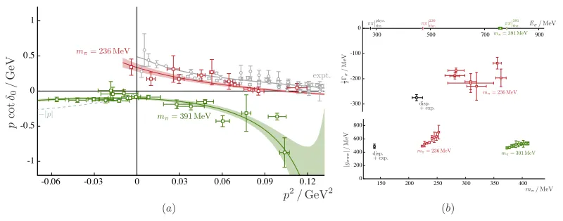
Figure 2. (a) Shown are the values of the pcotδ from Ref. [52] compared with the phenomenologi-cal/experimental values [17,53–56]. (b) Top panel shows the pole location of theσandσ →ππcouplings

from lattice QCD [52] and dispersive analysis of scattering data [17,57,58].

energies can, in practice, be extracted from two-point correlation functions,

C2pt.

ab (t,P)≡ 0|Ob(t,P)O†a(0,P)|0=

n

Zb,nZa†,ne−Ent, (4)

whereO†aandObare generic source/sink operators with the same quantum numbers.

In order to study resonances, it is necessary to map out the energy-dependence of the scattering amplitude and from it deduce its pole structure. This requires determining a large number of en-ergy levels, not just the ground states. This is arguably the most challenging aspect of this program. Fortunately, there has been a significant effort on this front [11,38–51], which have allowed one to

determine energies above multiple open threshold. In Sec.3.3I discuss an example of this in the isoscalar sector.

3.2 Elastic scattering processes

In lattice QCD calculations, this ideas have been primarily been put into practice in determining elastic scattering amplitudes. Arguably the first signal that the field is reaching a level of maturity was the study of the isovectorππscattering phase shift studied in Ref. [8]. There the authors used three different volumes, multiples boosts and irreducible representations (irreps) to constrain the scattering

amplitude at over 30 different energies in the elastic region. At the time, this was unprecedented

achievement which was followed by other successful studies [9,59–61].5

Unlike the isovectorππchannel, until recently the isoscalar channel has been virtually unexplored. Having the same quantum numbers of the vacuum, this is one of the most phenomenologically inter-esting sectors of QCD. Having completely disconnected diagrams, it is also one of the more compu-tationally challenging channels to explore via lattice QCD. Nevertheless, one given the technology briefly discussed above, it is now possible to calculate spectra in this sector. The first time this was

(6)

1

/

E? ⇡⇡/MeV

-30 0 30 60 90 120 150 180

0.08 0.10 0.12 0.14 0.16 0.18 0.20 0.22

0.7 0.8 0.9

1.00.08 0.10 0.12 0.14 0.16 0.18 0.20 0.22

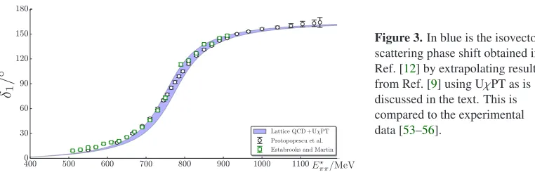
Figure 3.In blue is the isovectorππ

scattering phase shift obtained in Ref. [12] by extrapolating results from Ref. [9] using UχPT as is discussed in the text. This is compared to the experimental data [53–56].

done in a systematic fashion, without ignoring classes of diagrams and using an order of 10-30 op-erators for each irrep, was in Ref. [52] using two values of the light quark masses corresponding to

mπ =236,391 MeV.6

By restricting our attention to energies below theKKthreshold, Fig.2shows the resulting values of thepcotδ(proportional to the real part of the inverse of the scattering amplitude) for these two values ofmπ. These are compared to the experimental/phenomenological values [17,53–56]. Al-though a chiral extrapolation was not performed7_{, one observes a natural trend of these amplitudes as}

a function of the quark mass.

Having obtained the amplitudes, one can proceed to explore the pole content. For the heavier one finds a real pole below thresholds on the physical sheet, while for the lighter quark mass one finds a complex-valued pole on the second sheet above threshold. This is the manifestation of the σresonance for these quark masses. Once again, from Fig.2one finds a natural trajectory between these two points to the manifestation of the broad sigma in nature [17,57,58]. Furthermore, from the residue of the amplitudes one can obtain theσ→ππcoupling, which at this stage seems to have no to mild quark-mass dependence. Naturally, further investigation is needed, but this was the first evidence of theσfrom lattice QCD.

3.2.1 Chiral extrapolations

To this day, most calculations of resonances are being done using unphysically heavy values of the quark masses. The reason for this is multifold. With an increase in Wick contraction and the need of a order of magnitude increase in the basis of operators used, the computational cost of multiparticle observables far outweighs that of single-particle quantities. One can mitigate this cost by restricting to heavier quark masses. As we approach the physical point, we will need to increase the volume in order to keepmπL ∼4. This dramatically increases the density of states in the vicinity where we aim to determine the spectrum. This can be tackled with an even larger basis operators. An equally challenging problem emerges due to the fact that the energy cost for producing pion decreases as we approach the chiral limit. This would mean that in order to scan higher energies, where three or more particles can go on-shell, we would need a generalization of Eq.3(I come back to this in Sec.5).

While we proceed to tackle each one of these challenges, we can proceed to consider performing chiral extrapolations of resonant properties obtained at unphysically heavy quark masses. The natural tool for doing this would be chiral perturbation theory (χ PT), but at a finite orderχ PT does not exhibit a pole structure [65,66]. As a result, it is not suitable for describing resonance or bound states. A technique that enhances the range of applicability of theχPT is the so called the Inverse

(7)

1

/

E? ⇡⇡/MeV

-30 0 30 60 90 120 150 180

0.08 0.10 0.12 0.14 0.16 0.18 0.20 0.22

0.7 0.8 0.9

1.00.08 0.10 0.12 0.14 0.16 0.18 0.20 0.22

Figure 3.In blue is the isovectorππ

scattering phase shift obtained in Ref. [12] by extrapolating results from Ref. [9] using UχPT as is discussed in the text. This is compared to the experimental data [53–56].

done in a systematic fashion, without ignoring classes of diagrams and using an order of 10-30 op-erators for each irrep, was in Ref. [52] using two values of the light quark masses corresponding to

mπ =236,391 MeV.6

By restricting our attention to energies below theKKthreshold, Fig.2shows the resulting values of thepcotδ(proportional to the real part of the inverse of the scattering amplitude) for these two values ofmπ. These are compared to the experimental/phenomenological values [17,53–56]. Al-though a chiral extrapolation was not performed7_{, one observes a natural trend of these amplitudes as}

a function of the quark mass.

Having obtained the amplitudes, one can proceed to explore the pole content. For the heavier one finds a real pole below thresholds on the physical sheet, while for the lighter quark mass one finds a complex-valued pole on the second sheet above threshold. This is the manifestation of the σresonance for these quark masses. Once again, from Fig.2one finds a natural trajectory between these two points to the manifestation of the broad sigma in nature [17,57,58]. Furthermore, from the residue of the amplitudes one can obtain theσ→ππcoupling, which at this stage seems to have no to mild quark-mass dependence. Naturally, further investigation is needed, but this was the first evidence of theσfrom lattice QCD.

3.2.1 Chiral extrapolations

To this day, most calculations of resonances are being done using unphysically heavy values of the quark masses. The reason for this is multifold. With an increase in Wick contraction and the need of a order of magnitude increase in the basis of operators used, the computational cost of multiparticle observables far outweighs that of single-particle quantities. One can mitigate this cost by restricting to heavier quark masses. As we approach the physical point, we will need to increase the volume in order to keepmπL ∼4. This dramatically increases the density of states in the vicinity where we aim to determine the spectrum. This can be tackled with an even larger basis operators. An equally challenging problem emerges due to the fact that the energy cost for producing pion decreases as we approach the chiral limit. This would mean that in order to scan higher energies, where three or more particles can go on-shell, we would need a generalization of Eq.3(I come back to this in Sec.5).

While we proceed to tackle each one of these challenges, we can proceed to consider performing chiral extrapolations of resonant properties obtained at unphysically heavy quark masses. The natural tool for doing this would be chiral perturbation theory (χ PT), but at a finite orderχ PT does not exhibit a pole structure [65, 66]. As a result, it is not suitable for describing resonance or bound states. A technique that enhances the range of applicability of theχPT is the so called the Inverse

6_{In Sec.}_3.3_{, I discuss I discuss a recent extension of this work to higher energies for the}_m_π₌_{391 MeV ensembles [}₆₃_]. 7_{See Ref. [}₆₄_{] for first attempts to extrapolate these amplitudes.}

Amplitude Method [67–69]. The argument goes as follows. Let us impose force unitarity to be exact at all order in the chiral expansion. In other words, let the scattering amplitude satisfy Eq.1

M−1

UχPT ≡Re

M−1

χPT

−i 1

16π 2q

√_s Θ(s−s₀), (5)

whereMχPT is the standard amplitude obtained usingχPT andMUχPT is theunitarizedamplitude.

Going to the next-to-leading order (NLO) in the chiral expansion, and writingMχPT in terms ofMLO

andMNLO, we find

MUχPT=MLO_M 1

LO− MNLOMLO. (6)

0.10 0.12 0.14 0.16 0.18 0.20 0.22 0.24

16 20 24 16 20 24 16 20 24 16 20 24 16 20 24 0.10 0.15 0.20 0.25 0.30

16 20 24 16 20 24 16 20 24 16 20 24 0.10 0.12 0.14 0.16 0.18 0.20 0.22 0.24

16 20 24 16 20 24 16 20 24 16 20 24 16 20 24 0.10 0.12 0.14 0.16 0.18 0.20 0.22 0.24

16 20 24 16 20 24 16 20 24 16 20 24 16 20 24

(a) (b)

Figure 4. Shown are the finite-volume spectra obtained in Ref. [63] usingmπ = 391 MeV for the isoscalar

ππ,KK, ηηsector for irreps that primarily couple to (a)=0 and (b)=2 partial waves.

At this order, the isovectorππscattering amplitude is described in terms of two low-energy co-efficients (LECs). The same LECs describe both the quark-mass and energy dependence, which are

correlated withinχPT. Exploiting this correlation, Ref. [12] used NLO UχPT to fit the spectra ob-tained in Ref. [9] (shown in Fig.1). The resulting amplitude extrapolated to the physical point is shown in Fig.3, where one sees agreement with experiment [53–56]. Having the amplitude one can proceed to analytically continue and find theρpole, shown in Fig.1. In the same figure one sees agreement with poles obtained by using dispersive techniques to fit experimental data [13–18].

3.3 Coupled-channel systems:ππ,KK

(8)

0.2 0.4 0.6 0.8 1

800 1000 1200 1400

300 200 100

0.2 0.4 0.6 0.8 1

800 1000 1200 1400 1600

200 150 10050

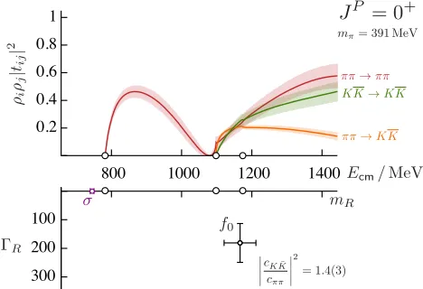
Figure 5.In the top panel are shown the modulus square of the three components of the S-wave scattering amplitude (tis proportional toMappearing Eq.1) describing the coupledππ,KKisoscalar

channels obtained in Ref. [63] using

mπ=391 MeV. Bottom panel shows the

poles of theσand f0resonances.

the two-point correlation function. One can adopt this procedure even when the amplitudes are not diagonal, i.e., when channels are coupled.8

These ideas were first put into practice for coupled channels in the study ofKπ,Kηscattering in the isodoublet channel usingmπ=391 MeV [72,73]. At these values of the quark masses, these two channels were practically decoupled. Similarly in Ref. [9]ππandKKwere found to be practically decoupled in the channel of theρ-resonances. The first strongly coupled calculations were performed in Refs. [74,75], and most recently this was put into practice in the isoscalar sector [63]. This study was an extension of the isoscalar calculations of Ref. [52], discussed in Sec.3.2.

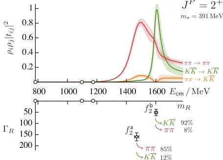
Reference [63] presented the finite-volume spectrum ofππ,KK, andηηin the isoscalar sector for themπ =391 MeV ensembles. The resulting spectrum, including a fit to it using one of a large range of parametrizations is shown in Fig.4. Although the spectrum is interesting on its own, the more interesting quantity to consider is the scattering amplitude. In Figures5 and 6show the different

components of the scattering amplitude, ignoring weak channels where theηηis present, in the=0

and = 2 partial waves respectively. Some prominent features of the S-wave amplitude is the fact

thatππandKKare very strongly coupled, similar to what is known phenomenologically. In addition to finding evidence of theσ, discussed above, these amplitudes show a clear signal of the resonance near theKK threshold. The location and relative coupling to the two channels is shown in Fig.5. Figure6shows the=2 partial wave amplitudes. As is evident, in this partial wave the two channels

are practically decoupled. Also, one sees two clearbump-likestructures. By exploring the behavior of these amplitudes in the complex plane, one finds the two resonances depicted in Fig.6.

4 Electroweak process from lattice QCD

In general, one would like study electroweak reactions involving scattering states in the initial and/or final state. This adds yet another source of complexity. If we are only interested in studying

reactions where the effects of the electroweak sector are perturbative, the most natural means to access

information of these reactions is by evaluating three-point functions with single insertions of the external electroweak current. In doing so, one can in principle extract finite-volume matrix elements

(9)

0.2 0.4 0.6 0.8 1

800 1000 1200 1400

300 200 100 0.2 0.4 0.6 0.8 1

800 1000 1200 1400 1600

200 150 10050

Figure 5.In the top panel are shown the modulus square of the three components of the S-wave scattering amplitude (tis proportional toMappearing Eq.1) describing the coupledππ,KKisoscalar

channels obtained in Ref. [63] using

mπ=391 MeV. Bottom panel shows the

poles of theσandf0resonances.

the two-point correlation function. One can adopt this procedure even when the amplitudes are not diagonal, i.e., when channels are coupled.8

These ideas were first put into practice for coupled channels in the study ofKπ,Kηscattering in the isodoublet channel usingmπ =391 MeV [72,73]. At these values of the quark masses, these two channels were practically decoupled. Similarly in Ref. [9]ππandKKwere found to be practically decoupled in the channel of theρ-resonances. The first strongly coupled calculations were performed in Refs. [74,75], and most recently this was put into practice in the isoscalar sector [63]. This study was an extension of the isoscalar calculations of Ref. [52], discussed in Sec.3.2.

Reference [63] presented the finite-volume spectrum ofππ,KK, andηηin the isoscalar sector for themπ=391 MeV ensembles. The resulting spectrum, including a fit to it using one of a large range of parametrizations is shown in Fig.4. Although the spectrum is interesting on its own, the more interesting quantity to consider is the scattering amplitude. In Figures5 and 6show the different

components of the scattering amplitude, ignoring weak channels where theηηis present, in the=0

and =2 partial waves respectively. Some prominent features of the S-wave amplitude is the fact

thatππandKKare very strongly coupled, similar to what is known phenomenologically. In addition to finding evidence of theσ, discussed above, these amplitudes show a clear signal of the resonance near theKK threshold. The location and relative coupling to the two channels is shown in Fig.5. Figure6shows the=2 partial wave amplitudes. As is evident, in this partial wave the two channels

are practically decoupled. Also, one sees two clearbump-likestructures. By exploring the behavior of these amplitudes in the complex plane, one finds the two resonances depicted in Fig.6.

4 Electroweak process from lattice QCD

In general, one would like study electroweak reactions involving scattering states in the initial and/or final state. This adds yet another source of complexity. If we are only interested in studying

reactions where the effects of the electroweak sector are perturbative, the most natural means to access

information of these reactions is by evaluating three-point functions with single insertions of the external electroweak current. In doing so, one can in principle extract finite-volume matrix elements

8_{For parallel}_/_{alternative e}_ff_{orts for extracting coupled-channel scattering amplitudes presented in this conference see [}₇₁_].

0.2 0.4 0.6 0.8 1

800 1000 1200 1400

300 200 100 0.2 0.4 0.6 0.8 1

800 1000 1200 1400 1600

200 150 10050

Figure 6.The top panel shows the same as Fig.5but for the=2 partial waves.

Bottom panel shows the poles of the two lowest lying resonances in this channel.

of these currents,

C3pt.

ab (tf,Pf;Pi,ti)≡ 0|Ob(tf,Pf)J(0)O†a(ti,Pi)|0 ∝Enf,Pf,LJ(0)Eni,Pi,L

₊

· · ·, (7)

whereEni,Pi,L

_{explicitly denote the finite-volume states and the ellipses denote contribution}

asso-ciated with overlap with other states. Being able to extract the matrix elements of a given state (even the ground state) has been a historical challenge. Recently, it has been demonstrated that in practice one can use the same techniques for extracting the excited state spectrum to also obtaining the matrix elements of the corresponding states [76].

Having then, in principle, determined such a matrix element, we must then understand how this matrix elements must be interpreted. When the initial and final states are stable under the strong interactions, these matrix elements are exponentially close to their infinite-volume counterparts

_E

nf,Pf,LJ(0)Eni,Pi,L

=Enf,Pf,∞J (0)Eni,Pi,∞

+Oe−mπL_. (8)

When the initial and/or final states are near or above a threshold, the relationship between this and

their infinite-volume counterparts are not obvious.

4.1 Interpreting1→2matrix elements

In recent years there has been substantial effort in developing the necessary formalism for studying

matrix elements involving two particles in the initial and/or final state. These ideas largely stem from

work developed by Lellouch and Lüscher explaining howK→ππweak decays can be accessed from the lattice [77]. These ideas have since been generalized to increasingly complex 0→2 [78,79], and 1 → 2 reactions [26,27,33,80–82]. In Ref. [83] the most general results for studying 0 → 2 and 1→2 transitions from finite volume matrix elements was presented. Although it turns out that these are closely, here I only discuss the latter.

Consider a current coupling a finite volume stateEn,PLto another stateE(1)₀ ,P,L. Here we

restrict our attention to the scenario where the latter correspond to a QCD stable state and where the volumes satisfymπL 1. This means we can assumeE(1)₀ ,P,L = E(1)₀ ,P,∞ up to negligible contributions. LetE2

n−P

₂₁_/₂

(10)

0 0

0 0.08

2.5 0.16

0.2 0.4 0.6 0.8

0 0.2 0.4 0.6 0.8

−2.5 2.0 2.1 2.2 2.3 2.4 2.5

2.0 2.1 2.2 2.3 2.4 2.5 2.0

0

0 50 100 4.0 6.0

(a) (b)

Figure 7. (a) Top panel shows theπγ _→ _ππ_{amplitude using} _m

π = 391 MeV as a function of the ππ

energy [84,85]. Bottom panel shows the elasticππamplitude for the same ensemble [8]. (b) Shown is the real and imaginary components of theπ_→ρform factor formmπ=700 MeV [76] andmπ=391 MeV [84,85].

Finally, we labelH to be the infinite-volume amplitude coupling the initial and final states. This amplitude is non-perturbative in the strong interactions but perturbative in the electroweak dynamics. We can write this amplitude as a vector in the degrees of freedom of the system, namely the partial waves of the two-particle state and the number of open channels open. With this, we can write a compact relationship between the finite-volume matrix element and the infinite-volume amplitude [83]

L3_E

n,PLJ(0)E(1)₀ ,P,∞= 1

2E₀(1)

HT_R₍_E_n_,_P₎_H_, ₍₉₎

whereRis the residue of the finite-volume two-particle propagator,

R(En,P)≡ lim E→En

(E−En) 1

F−1₍_P_,_L₎₊_M₍_s₎

. (10)

HereFandMare the same that appear in the quantization condition of the two-particle spectrum, Eq.3. In general, this is a matrix in the degrees of freedom of the two-particle channel. In the limit that a single channel is open and partial waves do not mix, only one component of this matrix would contribute, which is commonly referred to in the literature as the Lellouch-Lüscher factor.9

This equation can be explained as follows. Given the spectrum, one determineF,M, and conse-quentlyR. Next, one must determine the finite-volume matrix element using the standard three-point functions (arguably the most challenging task present). Once these are known one can use the map-ping defined by Eq.9to then obtained the desired infinite-volume amplitudeH.

4.2 πγ_→_ππ_{and the}_π_→_ρ_{form factor}

The formalism summarized above represents some of the first steps toward the lattice QCD com-munity being able say anything about the electromagnetic resonant processes. One of the first exam-ples of this was theγ_→_ππ_{amplitude obtained for the first time in Ref. [}₇₉_{] and now being explored}

9_{Although here we assume periodic symmetric volume, Ref. [}₈₃_{] presents a result that holds when the volume is asymmetric}

(11)

0 0

0 0.08

2.5 0.16 0.24

0.2 0.4 0.6 0.8

0 0.2 0.4 0.6 0.8

−2.5 2.0 2.1 2.2 2.3 2.4 2.5

2.0 2.1 2.2 2.3 2.4 2.5 2.0

0

0 50 100 4.0 6.0

(a) (b)

Figure 7. (a) Top panel shows theπγ _→ _ππ_{amplitude using} _m

π = 391 MeV as a function of theππ

energy [84,85]. Bottom panel shows the elasticππamplitude for the same ensemble [8]. (b) Shown is the real and imaginary components of theπ_→ρform factor formmπ=700 MeV [76] andmπ=391 MeV [84,85].

Finally, we labelH to be the infinite-volume amplitude coupling the initial and final states. This amplitude is non-perturbative in the strong interactions but perturbative in the electroweak dynamics. We can write this amplitude as a vector in the degrees of freedom of the system, namely the partial waves of the two-particle state and the number of open channels open. With this, we can write a compact relationship between the finite-volume matrix element and the infinite-volume amplitude [83]

L3_E

n,PLJ(0)E(1)₀ ,P,∞= 1

2E(1)₀

HT_R₍_E_n_,_P₎_H_, ₍₉₎

whereRis the residue of the finite-volume two-particle propagator,

R(En,P)≡ lim E→En

(E−En) 1

F−1₍_P_,_L₎₊_M₍_s₎

. (10)

HereF andMare the same that appear in the quantization condition of the two-particle spectrum, Eq.3. In general, this is a matrix in the degrees of freedom of the two-particle channel. In the limit that a single channel is open and partial waves do not mix, only one component of this matrix would contribute, which is commonly referred to in the literature as the Lellouch-Lüscher factor.9

This equation can be explained as follows. Given the spectrum, one determineF,M, and conse-quentlyR. Next, one must determine the finite-volume matrix element using the standard three-point functions (arguably the most challenging task present). Once these are known one can use the map-ping defined by Eq.9to then obtained the desired infinite-volume amplitudeH.

4.2 πγ_→_ππ_{and the}_π_→_ρ_{form factor}

The formalism summarized above represents some of the first steps toward the lattice QCD com-munity being able say anything about the electromagnetic resonant processes. One of the first exam-ples of this was theγ_→_ππ_{amplitude obtained for the first time in Ref. [}₇₉_{] and now being explored}

9_{Although here we assume periodic symmetric volume, Ref. [}₈₃_{] presents a result that holds when the volume is asymmetric}

with arbitrary twisted boundaries conditions.

by others [86]. These studies are partially motivated by the important role this amplitude plays in constraining the dominant hadronic contribution to anomalous magnetic moment of the muon.

A slightly more complicated process is γ_π _→ _ππ_{, which mimics the electro- and} photo-production reactions explored in, for example, the Thomas Jefferson National Accelerator Facility

(JLab). Given the important role played in the low-energy manifestation of QCD, it should not come as a surprised that this reaction plays an important role in a variety of processes, ranging from the chiral anomaly to the anomalous magnetic moment of the muon (see Refs. [87,88] for recent phe-nomenological studies of this amplitude).

The first study lattice QCD study ofγ_π_→_ππ_{was performed in Refs. [}₈₄_,₈₅_{]. This calculation} was done using the samemπ =391 MeV ensembles discussed above. In this study the γπ → ππ amplitude was determine for a range of energy of theππstate and virtuality of the photon. A global fit of this amplitude projected onto two virtualities and a range of energies is shown in Fig.7. One sees a clear manifestation of theρresonance, which coincides with its manifestation in the elasticππ amplitude.

By exploring the energy dependence of the this amplitude, one may obtain theπ→ρform factor. This can be defined in terms of the residue of the the amplitude at theρpole. This form factor is shown in Fig.7as a function of the virtuality for two values of the pion mass, one where theρis stable [76] and another when it is unstable [84,85].

5 Future prospects

Here I have attempted to give overview of the progress made in the studies of resonances on the lattice (for a more detailed review see Ref. [6]). I aimed to focus on ideas where there has been at least one application in a lattice calculation. Here I discuss what I believe might be three main areas of growth in future studies of resonance properties from lattice QCD.

Need for dispersive analysis: In right panel of Fig. 2we see the first determination of theσ resonance pole from lattice QCD. [52]. For the heavier ensemble, this turned to be a bound state. For the lighter ensemble, theσclosely mirrors the experimental one, meaning it appears as a broad resonance. In practice, this means that one must analytically continue amplitudes constrained on the real axis far into the complex plane. This is challenging problem, which explains why the mass of the σhas historically had such large systematic error. By choosing a different parametrization, one obtains

a different pole. This also explains why for themπ =236 MeV ensemble one sees a scatter of points in Fig.2. Phenomenologically, it is now well known that this systematic error can be greatly reduced by using a dispersive analysis of experimental scattering data [17,57,58]. This example clearly shows the need for a more sophisticated analysis of finite-volume spectra, where similarly ideas to those being used in modern-day amplitude analysis are adopted. Two other examples that illustrate the need for more sophisticated amplitude analysis are the coupled-channel systems (discussed in Sec.3.3) and three-body systems (discussed below)

Electroweak2→2processes and elastic form factors: Two classes of processes that are appar-ently accessible from lattice QCD but experimentally inaccessible are electroweak 2→ 2 processes and three-body scattering. Let me first discuss the former. These are amplitudes where a two-particle couples to an external current and then results in another or the same two-particle state. These am-plitudes, which are challenging to access experimentally, have been proposed in the literature for, for example, evaluating electromagnetic [90] and scalar [91] form factors of resonances.

(12)

partial wave amplitudes

two-to-two

matrix elements ₊

=

+

...

FV spectrum

one-body matrix elements

+ =

+

...

inÞnite-volume amplitude coupling two-hadron states to external current

elastic resonance form-factors

+

=

+

_...

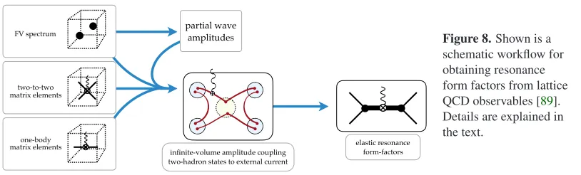
Figure 8.Shown is a schematic workflow for obtaining resonance form factors from lattice QCD observables [89]. Details are explained in the text.

was the first to derive a model-independent relation between such matrix elements and the corre-sponding amplitude.

The 2→2 amplitude,W, has kinematic singularities associated with intermediate particles going on-shell. The matrix elements are related to these amplitudes where the kinematic singularities have been exactly removed, resulting in the so-calleddivergence freeamplitude,Wdf. This can be related

to the finite-volume matrix element using the sameRdefined in Eq.10,

Enf,Pf,L|J(0)|Eni,Pi,L

2= 1

L6Tr

R WL,dfR WL,df, (11) WL,dfis related to the aforementionedWdf,

WL,df≡ Wdf+M G M, (12)

andGis a new finite-volume function that dependence on the spectrum and the single particle matrix elements.

This relation is similar to that appearing in Eq.9, and some the quantities needed are the same, namely the spectrum and R. The one main difference is this new finite-volume function G. As

was stated, this depend on the single particle matrix elements. This refers to the matrix elements of the constituents of the two-particle state. For example, if one would want to use this to study the ππJ → ππamplitude, one would also need to determine theπJ → π, to then use Eq.11. Figure8 summarizes the different ingredients needed to obtain the desired 2 → 2 amplitude. OnceWdf is

obtained, one can proceed to analytically continue onto the resonance poles of the incoming and final states, to extract elastic and/or inelastic resonance form factors. This is all to say that it is not

unfathomable to, in the not so distant future, study the structure of unstable states.

Three particles or more: All of the lattice QCD calculations of resonances have been restricted to states that couple solely to two-particles. This is in large part due to the fact that we do not yet understand, in general, how to extract three-body observables from finite-volume spectra. In recent years, there has been tremendous amount of progress with the aim of circumventing this problem [94– 104].10 _{Presently, the most general result for studying systems coupling to three-particles or less can}

be found in Ref. [101,104],

det

1+

F2 0

0 F3 KK322 KKdf23,3

=0. (13)

This quantization condition holds for energies where two- and three-particle states can go on-shell, and it gives a relationship between the spectrum and the infinite-volume K matrix. Unitarity relates the K matrix to the scattering amplitude, and Ref. [104] gives an exact relationship between these.

(13)

partial wave amplitudes

two-to-two

matrix elements ₊

=

+

...

FV spectrum

one-body matrix elements

+ =

+

...

inÞnite-volume amplitude coupling two-hadron states to external current

elastic resonance form-factors

+

=

+

_...

Figure 8.Shown is a schematic workflow for obtaining resonance form factors from lattice QCD observables [89]. Details are explained in the text.

was the first to derive a model-independent relation between such matrix elements and the corre-sponding amplitude.

The 2→2 amplitude,W, has kinematic singularities associated with intermediate particles going on-shell. The matrix elements are related to these amplitudes where the kinematic singularities have been exactly removed, resulting in the so-calleddivergence freeamplitude,Wdf. This can be related

to the finite-volume matrix element using the sameRdefined in Eq.10,

Enf,Pf,L|J(0)|Eni,Pi,L

2= 1

L6Tr

R WL,dfR WL,df, (11) WL,dfis related to the aforementionedWdf,

WL,df≡ Wdf+M G M, (12)

andGis a new finite-volume function that dependence on the spectrum and the single particle matrix elements.

This relation is similar to that appearing in Eq.9, and some the quantities needed are the same, namely the spectrum and R. The one main difference is this new finite-volume function G. As

was stated, this depend on the single particle matrix elements. This refers to the matrix elements of the constituents of the two-particle state. For example, if one would want to use this to study the ππJ → ππamplitude, one would also need to determine theπJ → π, to then use Eq.11. Figure8 summarizes the different ingredients needed to obtain the desired 2 → 2 amplitude. Once Wdf is

obtained, one can proceed to analytically continue onto the resonance poles of the incoming and final states, to extract elastic and/or inelastic resonance form factors. This is all to say that it is not

unfathomable to, in the not so distant future, study the structure of unstable states.

Three particles or more: All of the lattice QCD calculations of resonances have been restricted to states that couple solely to two-particles. This is in large part due to the fact that we do not yet understand, in general, how to extract three-body observables from finite-volume spectra. In recent years, there has been tremendous amount of progress with the aim of circumventing this problem [94– 104].10_{Presently, the most general result for studying systems coupling to three-particles or less can}

be found in Ref. [101,104],

det

1+

F2 0

0 F3 KK322 KKdf23,3

=0. (13)

This quantization condition holds for energies where two- and three-particle states can go on-shell, and it gives a relationship between the spectrum and the infinite-volume K matrix. Unitarity relates the K matrix to the scattering amplitude, and Ref. [104] gives an exact relationship between these.

10_{For development in 1}₊_{1 dimensional systems see [}₁₀₅_–₁₀₇_].

Unlike the two-particle analogue, Eq.3, this is not quite general. To this date all work involving three-particle states have assumed the individual particles to be identical bosons. This is a mild as-sumption, that could be easily removed. More restrictive is the fact that this equation only holds for kinematic regions where the two-body K matrix is non singular. This is a technical restriction that has not yet been surpassed. Once this formalism is complete, it is not hard to imagine being able to extend these ideas to study 1 → 3 transitions. This would be relevant for, for example, K → πππ weak decays andNγ_→_N_→_N_ππ_transitions.

6 Final remarks

We are entering an exciting era in hadronic physics. In the last few year, we have witnessed a tremendous amount of progress from the lattice QCD community in many fronts. One subfield that has surpassed its original expectations is the study of few-hadron resonant as well as non-resonant reactions. This field has been partly guided by formal ideas, some of which have been set forth over a quarter of a century ago, others that are being actively developed. But these formal concepts would be useless without the algorithmic and numerical developments.

Arguably, the algorithmic developments have surpassed the expectations of the more formal com-munity, which has now ignited a flurry of theoretical activity to explore processes that were previously believe to be inaccessible. This has in turn decreased the time period where ideas are being set out and when they put into practice. This is all to say that now is a perfect time to be working in these ideas, to develop them and immediately test them out in phenomenologically relevant calculations.

(14)

References

[1] K. Erkelenz, Phys. Rept.13, 191 (1974) [2] F. Hoyle, Astrophys. J. Suppl.1, 121 (1954)

[3] G.K.C. Cheung, C.E. Thomas, J.J. Dudek, R.G. Edwards (Hadron Spectrum) (2017),

1709.01417

[4] C. Hughes, E. Eichten, C.T.H. Davies, Submitted to: Phys. Rev. D (2017),1710.03236

[5] R.F. Lebed, R.E. Mitchell, E.S. Swanson, Prog. Part. Nucl. Phys.93, 143 (2017),1610.04528

[6] R.A. Briceno, J.J. Dudek, R.D. Young (2017),1706.06223

[7] V. Gribov, Strong interactions of hadrons at high energies: Gribov lectures on theoretical physics, Cambridge monographs on particle physics, nuclear physics, and cosmology (Cam-bridge Univ. Press, Cam(Cam-bridge, 2008),https://cds.cern.ch/record/1186219

[8] J.J. Dudek, R.G. Edwards, C.E. Thomas (Hadron Spectrum), Phys. Rev.D87, 034505 (2013), [Erratum: Phys. Rev.D90,no.9,099902(2014)],1212.0830

[9] D.J. Wilson, R.A. Briceno, J.J. Dudek, R.G. Edwards, C.E. Thomas, Phys. Rev.D92, 094502 (2015),1507.02599

[10] H.W. Lin et al. (Hadron Spectrum), Phys. Rev.D79, 034502 (2009),0810.3588

[11] J.J. Dudek, R.G. Edwards, P. Guo, C.E. Thomas (Hadron Spectrum), Phys. Rev.D88, 094505 (2013),1309.2608

[12] D.R. Bolton, R.A. Briceno, D.J. Wilson, Phys. Lett.B757, 50 (2016),1507.07928

[13] P. Masjuan, J. Ruiz de Elvira, J.J. Sanz-Cillero, Phys. Rev.D90, 097901 (2014),1410.2397

[14] B. Ananthanarayan, G. Colangelo, J. Gasser, H. Leutwyler, Phys. Rept. 353, 207 (2001),

hep-ph/0005297

[15] G. Colangelo, J. Gasser, H. Leutwyler, Nucl.Phys.B603, 125 (2001),hep-ph/0103088

[16] Z.Y. Zhou, G.Y. Qin, P. Zhang, Z. Xiao, H.Q. Zheng, N. Wu, JHEP 02, 043 (2005),

hep-ph/0406271

[17] R. Garcia-Martin, R. Kaminski, J.R. Pelaez, J. Ruiz de Elvira, Phys. Rev. Lett.107, 072001 (2011),1107.1635

[18] P. Masjuan, J.J. Sanz-Cillero, Eur. Phys. J.C73, 2594 (2013),1306.6308

[19] M. Luscher, Commun. Math. Phys.105, 153 (1986) [20] M. Luscher, Nucl. Phys.B354, 531 (1991)

[21] K. Rummukainen, S.A. Gottlieb, Nucl. Phys.B450, 397 (1995),hep-lat/9503028

[22] X. Feng, X. Li, C. Liu, Phys. Rev.D70, 014505 (2004),hep-lat/0404001

[23] S. He, X. Feng, C. Liu, JHEP07, 011 (2005),hep-lat/0504019

[24] P.F. Bedaque, Phys. Lett.B593, 82 (2004),nucl-th/0402051

[25] C. Liu, X. Feng, S. He, Int.J.Mod.Phys.A21, 847 (2006),hep-lat/0508022

[26] C.h. Kim, C.T. Sachrajda, S.R. Sharpe, Nucl. Phys.B727, 218 (2005),hep-lat/0507006

[27] N.H. Christ, C. Kim, T. Yamazaki, Phys. Rev.D72, 114506 (2005),hep-lat/0507009

[28] M. Lage, U.G. Meiner, A. Rusetsky, Phys. Lett.B681, 439 (2009),0905.0069

[29] V. Bernard, M. Lage, U.G. Meiner, A. Rusetsky, JHEP01, 019 (2011),1010.6018

[30] Z. Fu, Phys. Rev.D85, 014506 (2012),1110.0319

[31] L. Leskovec, S. Prelovsek, Phys. Rev.D85, 114507 (2012),1202.2145

[32] R.A. Briceno, Z. Davoudi, Phys. Rev.D88, 094507 (2013),1204.1110

[33] M.T. Hansen, S.R. Sharpe, Phys. Rev.D86, 016007 (2012),1204.0826

(15)