Group sequential testing of homogeneity in finite mixture models.

University of Windsor University of Windsor

Scholarship at UWindsor

Scholarship at UWindsor

Electronic Theses and Dissertations Theses, Dissertations, and Major Papers

1-1-2007

Group sequential testing of homogeneity in finite mixture models.

Group sequential testing of homogeneity in finite mixture models.

Yin Cui

University of Windsor

Follow this and additional works at: https://scholar.uwindsor.ca/etd

Recommended Citation Recommended Citation

Cui, Yin, "Group sequential testing of homogeneity in finite mixture models." (2007). Electronic Theses and Dissertations. 6982.

Gr o u p s e q u e n t i a l t e s t i n g o f h o m o g e n e i t y i n f i n i t e

M IX T U R E M ODELS

by

Y in Cui

A Thesis

subm itted to the Faculty o f Graduate Studies through M athematics and Statistics in P a rtial Fulfillm ent of the Requirements

for the degree of Master of Science at the U niversity of W indsor

W indsor, O ntario, Canada 2007

Library and Archives Canada

Bibliotheque et Archives Canada

Published Heritage Branch

395 W ellington Street Ottawa ON K1A 0N4 Canada

Your file Votre reference ISBN: 978-0-494-35007-2 Our file Notre reference ISBN: 978-0-494-35007-2 Direction du

Patrimoine de I'edition

395, rue W ellington Ottawa ON K1A 0N4 Canada

NOTICE:

The author has granted a non­

exclusive license allowing Library

and Archives Canada to reproduce,

publish, archive, preserve, conserve,

communicate to the public by

telecommunication or on the Internet,

loan, distribute and sell theses

worldwide, for commercial or non­

commercial purposes, in microform,

paper, electronic and/or any other

formats.

AVIS:

L'auteur a accorde une licence non exclusive

permettant a la Bibliotheque et Archives

Canada de reproduire, publier, archiver,

sauvegarder, conserver, transmettre au public

par telecommunication ou par I'lnternet, preter,

distribuer et vendre des theses partout dans

le monde, a des fins commerciales ou autres,

sur support microforme, papier, electronique

et/ou autres formats.

The author retains copyright

ownership and moral rights in

this thesis. Neither the thesis

nor substantial extracts from it

may be printed or otherwise

reproduced without the author's

permission.

L'auteur conserve la propriete du droit d'auteur

et des droits moraux qui protege cette these.

Ni la these ni des extraits substantiels de

celle-ci ne doivent etre imprimes ou autrement

reproduits sans son autorisation.

In compliance with the Canadian

Privacy Act some supporting

forms may have been removed

from this thesis.

T E S T IN G FO R H O M O G E N E IT Y IN F IN IT E M IX T U R E M ODELS IN GROUP SE Q U EN TIA L DESIGN

Y in Cui

Master of Science, 2007

Departm ent Mathematics and Statistics

University of W indsor

Abstract

The problem of testing wether a sample is from a homogeneous population has been

investigated in the recent years by many authors. I t has been recognized th a t the

lim itin g d is trib u tio n of the likelihood ra tio test for such homogeneity problems is very

complex and d iffic u lt to implement. Therefore, recently, Chen et al (2001) proposed

a modified likelihood ra tio test for homogeneity in finite m ixtu re models w ith general

parametric kernel d is trib u tio n families. In this thesis we provide a group sequential

version of this m odified likelihood ra tio test. The group sequential tests are often used

to reduce the sample size (number of observations) required for m aking decisions in

statistical testing. In general, group sequential procedures require less sample than a

fixed-sample (nonsequential) testing procedure w ith the same power and type I error.

We used Monte Carlo simulations to illu strate the performance of the proposed group

sequential procedures in the context of normal, binom ial and Poisson mixtures. We

apply the methods to a Poisson data set concerning the counts of number of accidents

Acknowledgments

I would like to gratefully acknowledge the enthusiastic supervision of my advisors

Dr. Hussein for helping me throughout my study at the University of W indsor and

valuable suggestions to this thesis. I especially wish to express gratitude to the

thesis reader Dr.Nkurunziza and Dr. Hubberstey for their continuous guidance and

Contents

List of Tables vi

List of Figures vii

1 Introduction 1

1.1 F in ite M ix tu re M o d e ls . . . . ... 1

1.2 Homogeneity Testing Problems ... 3

1.3 Group Sequential Testing P ro c e d u re s ... . 5

1.4 Thesis Objectives and O rg a n iz a tio n ... 7

2 Likelihood Ratio Test 9 2 . 1 O rdinary Likelihood Ratio T e s t ... 9

2.2 Drawbacks of the O rdinary Likelihood Ratio Test ... 10

2.3 M odified Likelihood Ratio T e s t ... 12

3 Group Sequential M L R T 15 3.1 In tro d u ctio n ... 15

3.2 General Group Sequential P roced ures... 16

3.3 A n Illu s tra tiv e E x a m p le ... 22

3.4 Group Sequential M L R T ... 24

3.4.1 Information-based Design.... ... 27

4 Simulations 30 4.1 Norm al and Poisson M ix t u r e s ... 30

4.2 Binom ial M ixtures: A p plication to Linkage A n a ly s is ... 35

5 Application and Concluding Remarks 64 5.1 A p plication to Accident D a t a ... 64

5.2 Conclusions and D iscu ssio n s... 67

Contents

Appendices 72

Appendix A: Five Regularity Conditions on Kernel Distribution 72

List of Tables

4.1 Parameters of the normal and Poisson models considered in the simu­

la tion s t u d y 33

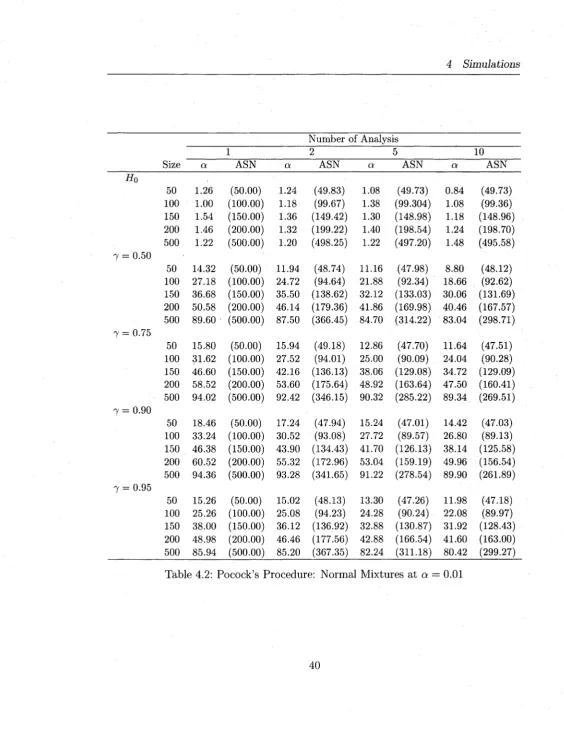
4.2 Pocock’s Procedure: Norm al M ixtures at a = 0 .0 1 ... 40

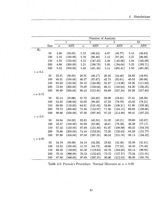
4.3 Pocock’s Procedure: Norm al M ixtures at a = 0.05 ... 41

4.4 Pocock’s Procedure: Norm al M ixtures at a — 0 .1 0 ... 42

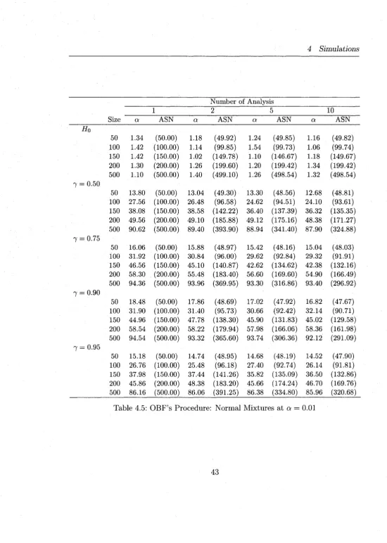
4.5 O B F ’s Procedure: Norm al M ixtures at a — 0.01 . . . 43

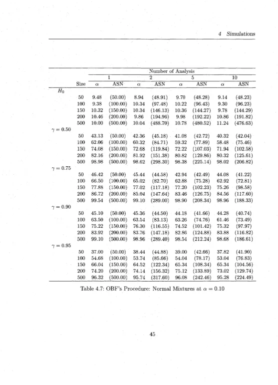
4.6 O B F ’s Procedure: Norm al M ixtures at a = 0.05 44 4.7 O B F ’s Procedure: Norm al M ixtures at a — 0.10 ... 45

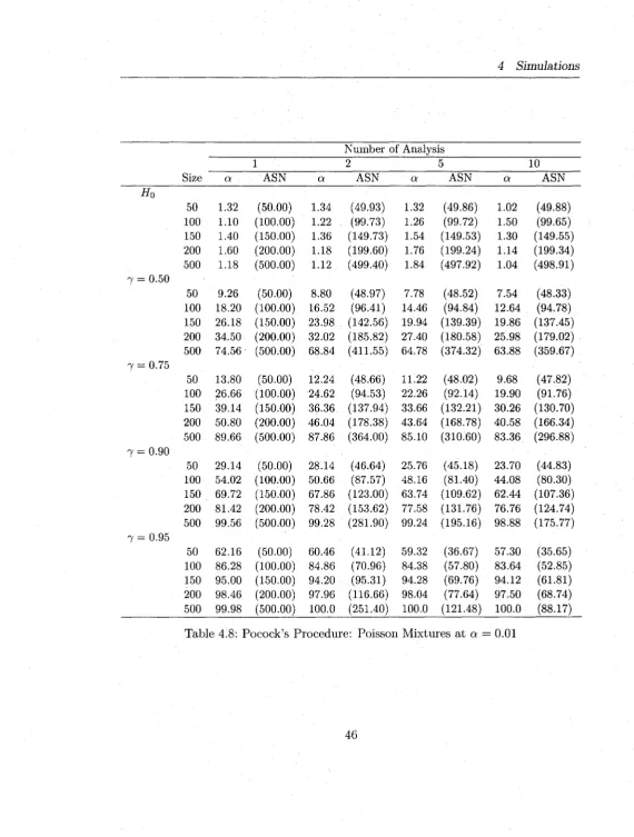
4.8 Pocock’s Procedure: Poisson M ixtures at a = 0.01 ... 46

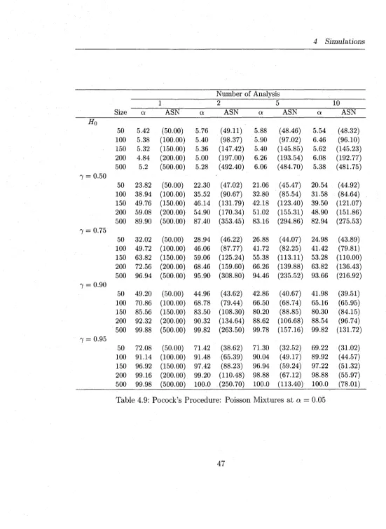
4.9 Pocock’s Procedure: Poisson M ixtures at a = 0.05 . . . . 47

4.10 Pocock’s Procedure: Poisson M ixtures at a = 0 .1 0 ... 48

4.11 O B F ’s Procedure: Poisson M ixtures at a = 0 . 0 1 ... 49

4.12 O B F ’s Procedure: Poisson M ixtures at a — 0 . 0 5 ... 50

4.13 O B F ’s Procedure: Poisson M ixtures at a = 0 . 1 0 ... 51

4.14 Pocock’s Procedure: Binom ial M ixtures at a = 0.05 m = 2 (P K ) . . . 52

4.15 Pocock’s Procedure: Binom ial M ixtures at a = 0.05 m = 4 (P K ) . . . 53

4.16 Pocock’s Procedure: Binom ial M ixtures at a = 0.05 m= 8 (P K ) . . . 54

4.17 Pocock’s Procedure: Binom ial M ixtures at a = 0.05 m = 2 (PU) . . . . 55

4.18 Pocock’s Procedure: B inom ial M ixtures at a = 0.05 m = 4 (PU) . . . . 56

4.19 Pocock’s Procedure: Binom ial M ixtures at a = 0.05 m= 8 (PU) . . . . 57

4.20 O B F ’s Procedure: Binom ial M ixtures at a = 0.05 m = 2 ( P K ) ... 58

4.21 O B F ’s Procedure: Binom ial M ixtures at a — 0.05 m = 4 ( P K ) ... 59

4.22 O B F ’s Procedure: Binom ial M ixtures at a — 0.05 m= 8 (P K ) . . . 60

4.23 O B F ’s Procedure: B inom ial M ixtures at a = 0.05 m = 2 ( P U ) ... 61

4.24 O B F ’s Procedure: B inom ial M ixtures at a = 0.05 m = 4 ( P U ) ... 62

4.25 O B F ’s Procedure: Binom ial M ixtures at a = 0.05 m= 8 ( P U ) ... 63

5.1 Number of accidents incurred by 414 machinists over a period o f 3 months ... 65

List of Figures

List of Acronyms

a.s. almost sure

ASN Average Sample Number

CDF Cum ulative D is trib u tio n Function

LRT Likelihood R atio Test

M LE M axim um Likelihood Estimate

M L R T M odified Likelihood R atio Test

OBF O ’Brien and Fleming

PD F P ro b a b ility Density Function

PK Phase Known

1 Introduction

1.1

Finite M ixture Models

Suppose X \ , . . . , X n are independent and identically distributed p-dimensional random

vectors w ith p ro b a b ility density function f ( x j ) on Mp. We say th a t X j are from a

finite m ixture population if the density f ( x j) can be w ritte n in the form

k

f ( xj ) = (1.1)

i= 1

where the f i ( x j ) are the densities and the % are nonnegative quantities th a t sum to

one. T h a t is:

k

0 < 7i < 1 ,i = 1,..., k and q* = 1.

*=l

The quantities q i , a r e called the m ixing proportions. The f i ( x j ) are called the

component densities or kernels of the m ixture.

F in ite m ixture models have provided a mathematical-based approach to the sta­

1 Introduction

models have been successfully applied include astronomy, biology, genetics, medicine,

psychiatry, economics, engineering and marketing. In these applications, fin ite m ix­

ture models underpin a variety of techniques in m ajor areas of statistics, including

cluster and latent class analysis, discrim inant analysis, image analysis, and survival

analysis. Here we w ill briefly review some examples where fin ite m ixtu re models are

found to be useful models. For a detailed and complete coverage of fin ite m ixture

models, readers are referred to the books of E v e ritt and Hand (1981) and McLachlan

and Peel (2000).

Linkage Analysis. Linkage analysis is a branch of human genetics th a t seeks the

assignment of genetic loci to particular chromosome regions, or linkage groups, by

the study o f th e ir cosegregation in families. Because of the wide availa bility o f D N A

polymorphism, linkage is now one o f the principal methods used to investigate genetic

diseases of unknown biochemical origin. W hen two genes (say, an unknown disease

gene and a known marker gene) are close to each other on the same chromosome, they

tend to stay in the same gamete after meiosis. The closer they are, the smaller the

chance of being separated. A gamete w ith only one of the two alleles is called recom­

binant and the recombination fraction, denoted as 9, is a useful measure of distance.

W hen 9 is close to 0, the two genes are tig h tly linked and located close to each other

on the same chromosome. W hen two genes are not linked, the recombination fraction

takes the m axim um possible value, 9 — 0.5. Sometimes, though, the underlying pop­

ulation is not homogeneous and the members of the population contain both linked

and unlinked members. In such case, a binom ial m ixture model is often used to test

1 Introduction

Cluster Analysis. Cluster analysis is an exploratory data analysis to o l for solving

classification problems. Its object is to sort cases in to groups, or clusters, so th a t the

degree of association is strong between members of the same cluster and weak between

members of different clusters. Each cluster thus describes, in terms of the data

collected, the class to which its members belong. M ixtu re models, usually Gaussian,

provide a useful statistical model for such clustering in many areas among which is

the recently expanding m icroarry data analysis.

Long-term survivor models. I t happens sometimes th a t a cohort of individuals whose

survival tim e is under study includes a group dying from a cause other than the

cause o f interest. In such cases, the analysis is handled by assuming th a t there is a

fraction of cured subjects whose failure tim e is at infinity, when it comes to the cause

of interest. T h a t is, the cohort under study is thought of as they were made up of

two sub-cohorts one following some sort of survival d istrib u tio n w ith respect to the

cause o f interest and the other as a cured sub-subcohort. Therefore, a two-component

m ixture model would be appropriate for carrying out this type of analysis.

1.2

Homogeneity Testing Problems

Often in clinical applications, one could ask the question whether observed data are

a sample from a single d istrib u tio n or whether they have come from several separate

distributions. For instance, a problem th a t frequently occurs in clinical tria ls is th a t

some subjects are less susceptible to the treatm ent than others are. A m ixture model

has tra d itio n a lly been proposed to describe the d istrib u tio n of responses in treatm ent

compo-1 Introduction

nents of complex human diseases. Researchers often rely heavily on the case control

association designs to investigate such complex diseases. However, they are often in

a dilemma as to whether they should recruit as many affected cases as they can in

a study, which, in these cases, may constitute a heterogeneous group, or whether

they should instead insist on a stricter case definition to achieve greater homogene­

ity. Testing for the homogeneity in this case w ill benefit both economics and design

purposes.

The likelihood ra tio test (LR T) is often used in param etric hypothesis testing.

Under standard regularity conditions, the LR T statistic has the simple and elegant

asym ptotic ^ -d is trib u tio n under the n u ll hypothesis (Lehmann 1999). U nfortunately

w ith m ixture models, regularity conditions do not hold for the LR T to have its

usual asym ptotic null d is trib u tio n of y2 w ith degrees of freedom equal to the d if­

ference between the number of parameters under the null and alternative hypotheses.

Ghosh and Sen (1985) considered the case of testing homogeneity against location-

contaminated norm al m ixtures w ith known variance. They showed th a t, under a

separation condition imposed on the parameter space, the likelihood ra tio test statis­

tic is asym ptotically distribu te d as a supremum of a Gaussian process w ith mean zero

and covariance kernel th a t depends on the true parameters under the n u ll hypothesis.

T itte rin g to n et al. (1985) consider the LR T of Ho : 7 = 1 versus H \ : 0 < 7 < 1,

where 7 is the m ixing proportion of a two-component m ixture. They derive that,

asym ptotically under H 0, the statistic follows a m ixture of y2 distrib u tio n , 5X0 +

where Xo denotes the degenerate d istrib u tio n th a t puts mass 1 at zero. A number of

1 Introduction

some of the parameters are known. Liang and Rathouz (1999) define a score function

which is sensitive toward a given alternative. This method also has a nice m athemat­

ical and statistical properties through choice of the alternative, which is somewhat an

a rb itra ry choice. Chen et al. (2001) propose a modified likelihood ratio test (M L R T )

for homogeneity in the fin ite m ixture models. The M L R T provides a nice solution to

this situation by sim ply adding a penalty term to the log-likelihood function. The

lim itin g d istrib u tio n of the M L R T statistic is a m ixture of chi-squared d istrib u tio n

for a large variety of m ixture models. In addition, it is asym ptotically most power­

fu l under the local alternative models when there are no structural parameters (i.e.,

nuisance parameters).

1.3

Group Sequential Testing Procedures

Statistical sequential testing methods were originated by Abraham W ald in the 1940s

during the second world war. They were invented in the context of in dustrial quality

control and the main purpose was to reduce the sample size required for making deci­

sion in statistical testing procedures. The first version of sequential testing procedures

was coined by W ald as Sequential P ro b a b ility R atio Test, SPRT. The name indicates

th a t a likelihood ratio test is being used in a sequential fashion. The SPRT opened

a century-long development in the field and quite many researchers worked in it. Se­

quential testing of hypotheses was introduced in to the biomedical and clinical trials

field during the 50s by Arm itage (1960). As an alternative to the SPRTs, Arm itage

et al. (1969) suggested and studied the so-called “ Repeated Significance Test” (RST).

cumu-1 Introduction

lative data every tim e an observation arrives. T h a t is, no conventional fixed-sample

tests w ill be performed if the to ta l sample size attainable at the end o f the study

is no- The n u ll hypothesis of interest is then rejected at the first inspection when

the conventional fixed-sample test rejects it. The critica l values, zai, i = 1,..., n 0,

used for the interm ediate testing, are obtained either by numerical integration as in

Arm itage et al. (1969) or from the approxim ating continuous tim e W iener processes

(Siegmund 1985).

Since, in double-blinded m ulti-centre clinical trials, frequent inspections may not

be feasible, Pocock (1977) introduced a “ group sequential” version of the RST. This

approach performs a repeated significance testing only periodically as opposed to

continuously testing after each observation. The conventional testing is performed at

the pre-specified inspection times, h , . . . , t K , w ith a fixed number o f patients (group

of patients) recruited between each two inspection times; th a t is, the number of

patients, n k — rifc_i, recruited between the i ^ q t h and A th inspection is same for all

k = 2,..., K . The critica l values, cak, k = 1,..., K , used for the interm ediate testing,

are all same and equal to a constant, c. This constant is computed from the jo in t

d istrib u tio n (exact or approximate) of the K conventional test statistics by requiring

th a t the overall significance level is a pre-specified Type Terror a, i.e.,

P {R e je ct Ho at any tk < tpc} = «•

O ’Brien and Fleming (1979) modified the constant boundary of Pocock’s original

group sequential method (i.e., cak = constant for all k < K ) to a square root

1 Introduction

Beta-Blocker Heart A tta ck Trial.

Lan and DeMets (1983) fu rth e r extended this methodology to accommodate un­

equal group sizes. The ir m onitoring tim e scale was the cumulative fraction of infor­

m ation obtained up to the tim e of the current analysis out of the to ta l inform ation

planned to be obtained at the end o f the study. T h a t is, if the m axim um inform ation

planned for at the end of the study is I k and I k is the inform ation obtained up to

the fcth analysis, then the fcth analysis takes place at the tim e t k = I kj I K . This

form ulation, w ith the help o f Brownian m otion approxim ation and an a-spending

function, gives group sequential methods which require neither equal group sizes nor

pre-fixed number of analysis K . For fu rth e r details account of group sequential sta­

tistica l inferences, we refer the reader to the monograph by Jennison and T urnbu ll

(2000).

1.4

Thesis Objectives and Organization

The objective of the thesis is to devise group sequential procedures for testing the

hypothesis th a t a population under study is homogeneous as opposed to being a two-

component m ixture. For this purpose, we use a sequential version of the modified

likelihood ra tio procedure of Chen et al. (2001). In chapter 2 o f this thesis, we review

the main results regarding the M L R T and the regularity conditions used to show its

asym ptotic properties. Chapter 3 reviews the various group sequential testing pro­

cedures th a t are commonly used in practice. Also, in chapter 3, we prove the main

result of the thesis in the form of Brownian m otion approxim ation to a continuous­

mo-1 Introduction

tion approxim ation is then used to construct various types of group sequential testing

procedures and th e ir m onitoring boundaries. In chapter 4 we report the results of

extensive Monte Carlo simulations to assess the performance of the proposed group

sequential tests in terms of type I errors, powers and average sample sizes needed to

detect genuine heterogeneity of mixtures. Three different density functions: Normal,

Poisson and Binom ial, are considered for the sim ulation experiments. In Chapter 5,

we apply some o f the proposed procedures to accident data from Greenwood and Yule

(1920), where the true model is suspected to be a m ixture of Poisson distrib u tio n ,

2 Likelihood Ratio Test

2.1

Ordinary Likelihood Ratio Test

Suppose we collected independent observations X 1, . . . , X n from a common density

(g (x ,9 ) : 9 £ © }, which is a p ro b a b ility density function (pdf) suspected to be a

m ixture o f two densities. T h a t is; we suspect th a t the p d f is o f the form

9 ( x ] l , 0 ) ■= ( 1 - ' y ) f ( x , 0 1) + 'y f { x ,d 2), (2.1)

where 9i < 02 € 0 and 0 < 7 < 1. To verify whether the density is of the form above

as opposed to being of the form f ( x , 9), one needs to statistically test the hypothesis

of homogeneity

Ho : 7 = 0 or 7 = 1 or equivalently 9i = 92

A ll o f the above equivalent n u ll hypotheses lead to the same conclusion th a t the

observations are from a homogeneous population w ith one common density of the

2 Likelihood Ratio Test

The ordinary log-likelihood function is given by

n

l n {7 , 0 1 , 0 2 ) = J > g { ( l + l f { X M ) ( 2 . 2 )

i—1

Let 7, 0 i,02 be the maxim um likelihood estimators of the parameters under the

whole param etric space : fIh q U , i.e., the maximizers of (2.2). Let also 6q be

the maximizer of Z „(l, 6q, #o) over the parameter space —oo < 60 < oo, i.e., m axim um

likelihood estim ator of population parameter 0 when the hypothesis of homogeneity

is true. Then the L R T is to reject the null hypothesis Ho if

■ R n = 2 { lnt f j 1,d2) - l n( l , d 0,90) } (2-3)

is large enough. The asym ptotic null d istrib u tio n of Rn is used to determine a critica l

value for the test. However, due to the irre g u la rity of the fin ite m ixtu re models,

the likelihood ra tio statistic R n does not have the usual y2 lim itin g distrib u tio n . The

article by Ghosh and Sen (1985) provide a comprehensive account of the breakdown in

regularity conditions for the classical asym ptotic theory to hold for the likelihood ra tio

test statistic. T itte rin g to n et al. (1985) give a more intensive discussion regarding

this problem.

2.2

Drawbacks o f the Ordinary Likelihood Ratio Test

2 Likelihood Ratio Test

asym ptotic d istrib u tio n of the L R T statistic for homogeneity H 0 is th a t of

{s u p IT + (0 ) } 2

0e©

where W (6) is a Gaussian process w ith mean 0, variance 1 and autocorrelation func­

tion

c m j Z M - h ( e ) Y , ( D ) , Z m - h ( m m n A , ^ v a r { Z , m - h (e )Y ,( 8 0) } v a r { Z , ( e ') - '

Here

Y( 0 \ Y( f f 0 i - ~ f ( X i ’ eo) n _ L n . y ( 0 \ Y ( ( j 0 N f ' { X i , 00) Y M - W M _ ( e _ e o ) m A ) , t # K Y M

-(2.5)

z m = Zi(e,e

0) =

e Z M = H o M

=

dYi{^

9

° \ e=%\

( 2 .6 )

and

E { Y m z m )

m ~ ~ w m r - ( ]

This asym ptotic result proves th a t the large sample behavior of the L R T is no

longer a y2 distribu tion. Chen et al. (2001) summarize the m ain drawbacks of the LR T

in these finite m ixture problems. As we could see from the (2.4-2.7), the asymptotic

2 Likelihood Ratio Test

Chernoff and Lehmann (1954) also raise this issue in Pearson’s y 2-test w ith presence of

nuisance parameters. Because o f this complicated asym ptotic d istrib u tio n presented

in the form of supremum of a Gaussian process, a simulation-based test is often used

to obtain critica l values for testing.

Finally, it is w o rth mentioning th a t the autocorrelation functions o f the lim itin g

Gaussian functionals, are different for different distributions. For example, Chen and

Chen (1998) showed th a t, if f ( x , 9) is a density of a N(6, a) w ith a = 1 9q = 0, 9 and

9' ^ 0, we have the autocorrelation

However, for a Poisson d istrib u tio n e e9x/ x \, x —1,2,..., the autocorrelation is

F irst one is th a t the null hypothesis 7 = 0 or 7 = 1 lies on the boundary of the

parameter space. The second complication is th a t 7, #1 and 92 are not identifiable

p{9,9')

e oe' _ 1 _ 00/

p(9,9>) = evl/ - 1 - m /

where

a a

v v 9 ' - 9

\/9~o

2.3

M odified Likelihood Ratio Test

2 Likelihood Ratio Test

under the null distribution. The main idea of the modified likelihood ra tio test is

to add an extra term in order to fix these two problems. The modified likelihood

ratio test based on the following modified log-likelihood function l'n(7, 0\,02) provides

a satisfactory solution. For 0 < j < l , 0 i , 0 2 E ® w ith 01 < 02, Chen et al. (2001)

defined modified log-likelihood function as,

n

4 (7 , Ou e2) = lo g { ( l - 7 00 + 7f ( X i , 0 2) } + C lo g{47 ( l - 7) }, (2.8)

i= 1

where the constant C > 0 is used to control the level of m odification to the log-

likelihood function. Notice th a t in this form ulation the values of 7 — 1 and 7 = 0 are

excluded from the parameter space, however, the n u ll hypothesis of homogeneity is

now o f the form Hq :7 = 1/2.

Let (7 ,0i, 02) maximize 4 (7 , 0^, 4 ) over the fu ll parameter space, Q : Q# 0 U

and let 0O maximize the null modified likelihood function 0o, ^0), ^ 0 € 0 . The

M L R T rejects the null hypothesis H 0 for large values of

M n = 2{l'n ^ A A ) - l ' n { \ A A ) } (2.9)

The additional term C lo g {4 7( l —7) } in equation (2.8) is non-positive and is intended

to discourage fits th a t result in values of 7 th a t are close to either 0 or 1. In fact,

we observe th a t the m odification term explodes to negative in fin ity whenever 7 is

close to 0 or 1, thus solving the problem of the boundary during the estim ation of

the parameters and hopefully m aking the likelihood behave more tractably.

2 Likelihood Ratio Test

must be met in order to establish the lim itin g d istrib u tio n of the M L R T statistic.

(Appendix A contains these conditions). The ir main result is th a t, if conditions 1-5

in appendix A hold, the asym ptotic null d istrib u tio n of the M L R T statistic M n is the

m ixture o f x i and Xo w ith equal weights, i.e.,

2%o + 2 * 1 (2-10)

where Xo is a degenerate d istrib u tio n w ith all its mass at 0.

Chen et al. (2001) suggested C = lo g (M ) as an appropriate choice when the

parameter 0 is in the interval [—M , M ] for some large constant M . For instance, this

could be the case when dealing w ith a practical problem in which the investigator can

reasonably assume th a t the parameter w ill fa ll in a certain interval. However, based on

the simulations done by Chen et al. (2001), the lim itin g d istrib u tio n of the modified

likelihood ra tio test is not very sensitive to the choice of C. Also, to improve the

lim itin g d istrib u tio n for small samples, Chen et al. (2001) suggested the use o f pn =

Ph0 ( M n < 0) as the weight for the degenerate chi-square in the lim itin g distribu tion. The authors showed th a t the M L R T is asym ptotically most powerful under the local

alternatives (alternatives th a t are close to the null hypothesis). Through Monte Carlo

simulations they also compared th e ir M L R T to Neyman’s C (a ) test, the bootstrap

test by McLachlan (1987) and the method o f Davies (1987), and they found th a t the

results o f the M L R T are the most promising. Therefore, the M L R T is a reasonable

3 Group Sequential M L R T

3.1

Introduction

Since last century, group sequential analysis has drawn great atte ntion in clinical

trials, epidemiological studies, q u a lity control and safety studies. Group sequential

experimentation is an area of statistics which is both o f practical im portance and

also of great theoretical interest. Group sequential statistical analysis was originally

developed to obtain economic benefits. E a rly stopping w ith positive results implies

th a t the new product can be in market sooner whereas if a negative result is indicated,

early stopping ensures th a t resources are not wasted. Group sequential methods

typ ica lly lead to savings in sample size, tim e and cost in comparison to fix-sample

(i.e., nonsequential) methods.

For ethical as well as practical reasons, investigators may wish to m onitor a study

and review it over tim e at in te rim looks to assess whether the research hypothesis is

sufficiently supported to warrant early term ination of the study. In a group sequential

study, a test statistic is typ ica lly computed at each look and compared to a stopping

3 Group Sequential M LRT

some predetermined overall significance level. In order to design and m onitor this

type of study, the jo in t d istrib u tio n of the sequentially computed statistics must be

derived.

In section 3.2, we review the commonly used group sequential m onitoring proce­

dures w ith greater emphasis on the so called alpha-spending approach o f Lan and

DeMets (1983). Section 3.3 provides a simple group sequential study to help reader

gain more understanding of the group sequential design. In section 3.4, we give the

main result th a t the m odified likelihood ratio test statistic behaves like a functional

of a Brownian m otion process and hence we illu strate how th is result can be used to

build m onitoring boundaries, in particular, the Lan-Demets boundaries.

3.2

General Group Sequential Procedures

In general, a group sequential design w ith K planned in terim analyses for testing the

hypothesis H 0 : 7 = 0 yields a sequence of test statistics { Z L. .... Z kj . We say th a t

this sequence o f statistics has the canonical jo in t distribution w ith inform ation levels

{ /1, ..., R } for the parameter 7 if:

• ( Z i , .... Zk) is m ultivariate normal,

• E ( Z k) = 7 \ / 4 , k = 1,..., K , and

• C o v(Zk l, Z k2) = \ J I kl /h 2 j 1 < h < k 2 < K

This jo in t canonical d istrib u tio n can often be shown to hold by approxim ating the

3 Group Sequential M LRT

points t i , t K ■ These tim e points are usually given in the so called inform ation tim e

scale, tk — h / l K i where /*, is the inform ation about the parameter of interest collected

up to the analysis k and Ik is the inform ation planned to be collected by the end of

the study. The tim e points represent for each k, the fraction of inform ation collected

by the fcth analysis. In many cases it can be shown th a t this fraction is approxim ately

the same as the fraction of sample size collected up to the k ih analysis, out of the

to ta l sample planned by the end o f the study.

For example, suppose it is required to test a null hypothesis Hq : 7 = 0 versus

Ha '■7 7^ 0. We consider group sequential tests in which up to K analysis are

perm itted and standardized statistics Zk, k =■T , ..., K , are available at these analysis.

I f the sequence of statistics follows the canonical jo in t d istribu tion, then we can easily

compute m onitoring boundaries ± C i, ..., i c K which satisfy a given type I error rate, a,

by using numerical integrations th a t exploit the canonical jo in t d is trib u tio n structure.

If, on the other hand, the canonical jo in t d istrib u tio n does not hold, then com put­

ing the m onitoring boundaries would require m ultivariate integrations th a t are highly

com putationally expensive even for number of analysis as large as K = 7.

There are many ways of choosing the boundaries ci, ...,c ^ , and in the next sub­

sections we are going to review some boundaries th a t are commonly used in practice.

We assume th a t the sequence of test statistics reject H 0 in favor of the alternative

hypothesis only for large values o f the test statistics.

Pocock’s Procedure

3 Group Sequential M LRT

significance level to analyze accumulating data at a relatively small number of times

over the course of an experiment. This is the simplest group sequential procedure in

the sense th a t it has constant m onitoring boundaries (straight lines). This procedure

assumed equal sample between analysis.

Formally, the test procedure is as follows:

• A fte r group k = 1,..., K — 1 (w ith cumulative sample ny.)

— if \Zk\ > CP( K , a), stop and reject Ho

— otherwise, continue to group k + 1

• A fte r group K

— if \Zk\ > Cp( K , a ) , stop and reject Hq

— otherwise, stop and accept H 0

The c ritic a l value CP( K , a ) is chosen to give a pre-fixed overall Type I error a,

i.e.,

P7=o{Reject Ho at stage k = 1, k = 2,..., or k = K } = a.

The Pocock’s procedure results in a constant boundary, independent o f the analy­

sis, K . This constant boundary value is tabulated for various a and K (see Jennison

and T urnbu ll (2000)). The Pocock’s method is not based on any form al optim al prop­

erties such as m inim izing sample size under some particular hypothesis. However, it

is rational and easy-to-use form of stopping rule which gives the test an im p o rta n t

3 Group Sequential M LRT

O ’Brien & Flem ing’s Procedure

O ’Brien and Fleming (1979) proposed a test in which the nom inal significance levels

needed to reject H 0 at each analysis increase as the study progresses. Thus, it is more

d ifficu lt to reject Ho at the earliest analyses b u t easier later on as the inform ation

available increases.

Consider the same experiment setup as in Pocock’s Procedure, and assume th a t

the sample sizes between analysis are equal. The O ’Brien-Flem ing test has the fol­

lowing algorithm

• A fte r group k — 1,..., K — 1 (w ith cumulative

— if \Zk\ > Cb(K , o t ) y / K / k , stop and reject Ho

— otherwise, continue to group k + 1

• A fte r group K

— if \Zk \ > Cb{ K ,ol), stop and reject H 0

— otherwise, stop and accept Ho

Since Cb(K , o t ) ^ j K / k decreases w ith increasing k, the O ’Brien-Flem ing test has

narrower boundaries at later analysis and hence, it is easier to reject H 0 at later

analysis than at early analysis.

E rro r Spending Procedure

As both the Pocock and O ’Brien & Fleming methods require equally spaced sam­

3 Group Sequential M LRT

m onitoring process. In other words, m odifying the times of analysis (say in the tim e

scale of inform ation fraction) or even reducing or increasing the frequency o f interim

analysis after the design stage, is not allowed. A violation o f these assumptions leads

to lower power and some times inflated type I error. To overcome such difficulties,

Lan and DeMets (1983) proposed a flexible m onitoring procedure known as the

a-spending (or error-a-spending) function approach. The procedure requires only the

specification, in advance, of an increasing function «(£), which characterizes the rate

at which type I' error, a, is spent.

Suppose the m axim um number of analysis, K , is fixed before the study, and

the Type I error is partitioned in to probabilities a i , . . . , a x , which sum to a. As

inform ation tim e f i = I \ / I k - , ■ ■ ■ • t x — I k / I k = 1 progresses, the two-sided critica l

values Cfc for the standardized statistics Z tk, k = 1,..., K , are calculated such th a t,

^ 5 ***7 \Htk — ll ^ Ck—1; — Cfc)" Qffc

Here, the Type I error is partitioned according to an error spending function a ( t),

which is non-decreasing and satisfies a(0) = 0 and a (t) = a, for t > 1. The value of

a ( t ) indicates the cum ulative Type I error th a t is to be spent when a fraction t of the

maximum anticipated inform ation has been obtained. The error spending function

and the target inform ation level must be decided before the design stage before the

3 Group Sequential M LRT

The Type I errors allocated to each analysis are

c*i = a ( ti) (3.1)

Oik = oi[tk) - a'(ife-i), k = 2,3, ...K (3.2)

C ritica l values ck are computed successively to satisfy (3.2) by using numerical inte­

gration th a t exploit the canonical jo in t d istrib u tio n of the test statistics. Equivalently,

the cumulative error can be used to compute the boundaries

k

a k = a ( t k) = ^ 2 p { \ z t i \ < c i , . . . , |Z t i _ x \ < C i - i , |Z t i \ > C i \ H 0 } .

i = 1

There are several a-spending functions proposed in the lite ra tu re which result in

various boundary shapes. There is no one best function, and often investigators use

a-spending functions th a t approxim ate well the two well-known procedures of Pocock

and O ’Brien-Fleming. For instance, the function

a ( t) = a t p, (3.3)

where p > 0 is a tunin g parameter which controls the shape of the boundary, is

studied in Lan and DeMets (1983). For p — 1 we get a boundary th a t mimics Pocock’s

boundary, whereas, p = 2 results in a boundary sim ilar to th a t of O ’Brien-Fleming.

The algorithm for m onitoring a group sequential testing procedure is, thus, not

3 Group Sequential M LRT

3.3

An Illustrative Example

In a typical two-arm randomized clinical tria l, subjects are recruited and divided

into two groups, a control group A and an experimental group B. Suppose th a t, on

the basis of a norm ally distributed response and a known common variance cr2, we

are interested in testing the null hypothesis of the equality of the means o f the two

populations, Hq : p a ~ AtB = 0, w ith overall significant level a = 0.05 versus the

alternative hypothesis H a : \/j,a — Pb\ = £ w ith power 1 — (3. Suppose the maxim um

projected sample size is 60 on each arm w ith 4 in terim looks, the testing procedure w ill

be carried out based on a two-sided O ’Brien-Flem ing boundary computed through the

a-spending function a t 2 = .05f2. I f we adopt a m onitoring schedule w ith equal sample

size increments at each analysis, then we should perform our analysis at the times

when n i = 30, n 2 = 60, n :i = 90 and = 120 cumulative sample sizes are available or

equivalently, on the inform ation fraction tim e scale, at times t \ = 30/120 = .25,1,2 =

.5, ts — .75, £4 = 1. The test uses the follow ing standardized statistic after each group

o f observations,

Zk = — . =

y j 4o2/rik

where k = 1 ,...,4 and X r\k and X s k are, respectively, sample mean for group A

and B based on the cumulative data collected on each group up to the analysis k.

The corresponding boundary values are {±4.408, ±2.862, ±2.337, ±2.204}. The upper

and lower arms of Figure 3.1 illu stra te these boundaries at the four analysis times.

Suppose th a t after the first analysis, our data gives a standardized test statistic w ith

3 Group Sequential M LRT

the value 0.711 for the first 15 subjects. The test statistic Z\ falls in the continuation

region so, we continue data collection and we prepare for the second analysis. Suppose

th a t the test statistic Z^ at the second analysis has a value of 2 . 2 0 1 and is s till

w ith in the continuation region. Thus, 45 subjects are collected in order to do the

th ird analysis. A t the th ird stage, we have a statistic Z% w ith a value of 2.685 and

the procedure rejects the n u ll hypothesis. Therefore, we stop the whole study and

conclude our result th a t there is a significant difference between Group A and Group

B in th e ir mean responses. The design boundaries and testing statistics at each

analysis are displayed in Figure 3.1.

- 1 - K=4

Function:0’Brien-Fleming Type, alpha=0.05

N

•e₀₎

Q-C

CM

0.4 0.6 0.8 1.0

Times

3 Group Sequential M LRT

3.4

Group Sequential M L R T

For the purpose of group sequential m onitoring, it is sufficient to show th a t the finite

dimensional d is trib u tio n of a continuous processes, converge to those o f a standard

Brownian m otion and th a t the M L R T is a some tractable function o f such a process.

The Brownian m otion process has independent increment structure and jo in t m u lti­

variate normal d istrib u tio n at any given set of K tim e points t i, .... t Kl as required

by the general setup o f group sequential methods described in the previous section.

Therefore, the M L R T w ill also benefit from such canonical structure and the moni­

toring boundaries can then be computed by using the usual numerical integrations.

We define a weighted and continuous version of the M L R T statistic as for

n = 1,2, 3 , . . . where t € (0,1], [nt] is the integer p a rt of n t and n is the final sample

size planned at the end of the study. This is sim ply a weighted interpolation of the

modified likelihood ra tio test M n. I t has been shown by Chen et al. (2001) th a t

( ( E I U m ) + )2

nE[W%] + ° v i 1)

where W* = Z{ — hYi and h = E [ Y Z \ / E [ Y 2]. The quantities Y, — Y ( 9 0) and Z i =

Zi(6o) are defined in Section 2.2. The random variables Wt have mean zero and

variance E [ W 2}. Under the null hypothesis, H 0, and in virtu e of condition 4 in the

appendix, it is easy to see th a t

3 Group Sequential M LRT

i.e., the random variables W* have fin ite variance. B y noticing th a t [nt] j n —> t as

n —> oo, we can w rite the above approxim ation in terms of the interpolated M L R T

process as follows,

[nt]

n

i £1

Wi X

+ ° p ( ! )

For sim p licity o f notations, p u t ^ = Wi

y /E W ? , which are i.i.d random variables w ith

mean 0 and variance 1, and w rite the interpolated and normalized p a rtia l sum process

M

s ”

= -7hX>

^ i—1

Now, classical results on convergence in d istrib u tio n for random measurable functions

on [0,1] apply. In particular, Donsker’s theorem (Billingsley 1968), states th a t, as

n oo, SJ* V B (t), where B ( t ) is a standard Brownian m otion on the interval

[0,1]. Furthermore, since the function h(x) = ) 2 is continuous, it follows th a t

such convergence s till holds under the the transform ation h(.) so th a t

fc(ST) = [(s ? )+)+ 1 2 ® [.B ( t)+F

As a consequence, the finite dimensional distributions of [(S' " ) " 1-] 2 converge to those

3 Group Sequential M LRT

are fixed tim e points, then

( [ ( S , ” , ) + ] 2 ...[ < s y + ] 2 ) — ( [ ( B ( t , ) ) + ] 2 , . . . , [ ( B f e ) ) + 1 2 ) .

Now, since n /[n t] —> 1 / t as n —»■ oo, by using the m ultivariate version o f Slutsky’s

theorem (Theorem 5.1.6 in Lehmann (1999, p.283)) and the Cramer-W ald device (see

Lehmann (1999)), one can show th a t

n o n n t i p 1

n o n [ntK \ K

v

2

' { B ( t K ) \ +'

\ V h ) _ ? • * * 5

as n —> oo. In summary, by setting r ik /n = tk where n*, is the sample size up to the

analysis k and n is the sample size at the end of the study, we can state the following

result:

T h e o r e m 1 Assume that conditions 1-5 in the appendix and Hq hold, and let 0 <

t i < t2 < ■ • ■ , < t x be some fixed time points in the interval [ 0 , 1 ] f o r k = 1 ,..., K (fixed

as n —> oo). Then the modified likelihood ratio test process, M t = M [nt] defined above

has its finite dimensional distributions converging to those of the squared positive part

of standardized Brownian motion. That is,

( Mt l , . . . , M tK) v ba

i₂

( B ( t K ) \ +'

i

> • • • i

*

1

3 Group Sequential M LRT

3.4.1

Information-based Design

As mentioned above, in a group sequential study designed according to an a-spending

function approach, has three steps to follow. F irst, one has to specify an overall

p ro b a b ility o f type I error,a, and the to ta l sample size needed for atta ining certain

desired power. Secondly, one has to decide the boundary type, which depends on

the o-spending function, and the times of analysis, which are usually equally spaced

in the sense th a t the analysis are performed at equal sample size increments. The

th ird step is to compute the m onitoring boundaries and start collecting the data. I f

the analysis times are modified along the way one has to m odify the current and the

future boundaries to adjust for the changes. These steps can also be form ulated in

the context of testing homogeneity of a m ixtu re using the M L R T and w ith the help

of the above theorem.

Suppose th a t we plan a group sequential study for testing the homogeneity in finite

m ixture models based on K in te rim analysis. Suppose th a t these in terim analysis

are planned at tim e points 0 = to < £i, • • • > < t x = 1 when rii, . ..,n x cumulative

samples are collected. Suppose also th a t we intend using a boundary based on a (t),

an a-spending function. As we mentioned earlier, a (t) gives the cumulative portion

o f the Type I error th a t has been spent on or p rio r to the fcth in te rim analysis. The

boundaries, Ci, c2, . . . , ck for m onitorin g the M L R T statistic at the in te rim analysis can be computed from the equations

k

Oil + ••• + a k = a (tk) = £ P { M tl < c i , . . . , M ti_j < > Ci\H0} (3.5)

3 Group Sequential M LRT

for k = 1 , 2 , . . . , K and M ti is the M L R T value computed at tim e ti, i.e., when there is

rii cumulative sample collected of the to ta l n planned for. B y using the approxim ating

positive-part Brownian m otion process defined in the theorem, this is almost the same

as m onitoring the process \ B + {tk) / and therefore,

a (tk)

fc-i

E p

i ~ 1

k- 1

= £

p

f B + (t i)

1 I

< Cl,

< y/ci, ■ ■ ■

B + (U . i)

\ / t i- 1

^ Cj _i , > C,;|#0

£ + ( L - i)

y / L - i

B + ( D

V u

- V " r rrr E Q iz i l <- /tt— > / r i H \ (o

> v ^ | L T o y (3.6)

7)

The second equality, (3.6), is obvious and the th ird one, (3.7), follows by arguing th a t,

since the numbers ct are all s tric tly positive, the origin of the if-d im e n sio n a l Euclidean

space is always excluded from the volume of interest by the restriction > ^/c~.

Therefore, the parts of the area o f interest where some coordinates are negative and

which, under the positive-part function, are collapsed to the hyperplanes defining

the positive orthant can be thought of as being expanded back and hence, as giving,

along w ith the volume in the positive orthant, the original volume under a m ultivariate

normal density o f the type given above. Thus, m onitoring the process [_B+ (tk)/ a/Pc] 2

is same as m onitoring B ( t k ) / \ / t k• The im portance of (3.7) is th a t we can sim ply

use the tabulated critica l values for the known group sequential procedures such as

Pocock and O BF procedures or any software th a t produces m onitoring boundaries

based on a-spending functions. For instance, if we were to conduct a group sequential

3 Group Sequential M LRT

level o f a — 0.05, then the desired constant boundary would be c = C'p(O.l), where

Cp(O .l) is the Pocock boundary corresponding to the m onitoring of a Z-score at level

a — 0.1.

In summary, the steps followed in designing the usual group sequential designs can

also be followed in testing homogeneity of m ixture via a group sequential M LR T .

4 Simulations

In order to assess the performance of the group sequential modified likelihood ra tio

test proposed in the previous chapter, we conduct several Monte Carlo simulations.

The first two of these Monte Carlo simulations follow the same setups as in Chen et al.

(2001) and they use Norm al and Poisson m ixture models. A p a rt from the n u ll models

(where homogeneity is assumed) four normal and four Poisson m ixtures w ith different

parameters are considered under the alternative hypothesis of non-homogeneity. The

th ird sim ulation considers the binom ial m ixture models arising from genetic linkage

analysis. We briefly introduce the background of the linkage analysis and relate our

problem as testing the homogeneity in the binom ial mixtures. The discussed phase

known and phase unknown situations are both considered w ith various parameter

settings.

4.1

Normal and Poisson M ixtures

The most im p o rta n t class of finite m ixture densities is the class of normal mixtures.

inci-4 Simulations

dental. One of the reasons is th a t a univariate normal d istrib u tio n has a simple and

concise representation requiring only two parameters, the mean p and the variance

<72. The norm al density is symmetric, unimodal, and assumes the least p rior knowl­

edge in estim ating an unknown p ro b a b ility density w ith a given mean and variance.

These characteristics along w ith its well-studied status give norm al m ixture density

models the power and effectiveness th a t other m ixtures can hardly surpass. Fields in

which norm al m ixture models are used are various ranging from genetics (Schork et

al. 1996) to the study of sensitivity of medical screening tests (McDonnell et al. 1998),

in the absence of gold standard, to machine learning applications. W ith in the statis­

tica l methodology, normal m ixture models have been used in the investigation of the

performances of certain estimators to departures from norm ality and in the develop­

ment o f robust estimators. Examples of many other areas where norm al m ixtures are

applied can be found in McLachlan and Peel (2000).

The Poisson m ixtures are used in many practical situations. Tw o im p o rta n t areas

of applications for the Poisson m ixtures are the modeling of over- or under-dispersion

and zero-inflation in count data. Often, count data (m ostly in toxicological, biological

and medical data) are modeled as if they were coming from a Poisson d istrib u tio n

w ith certain mean (or rate). A n im p o rta n t assumption o f the Poisson d istrib u tio n is

th a t the mean and the variance are equal. D ata sets in which evidence against mean-

variance equality is present are called over- or under-dispersed. One way of dealing

w ith such data is to fit a m ixture o f Poisson distributions w ith continuous m ixing

variable distributed as Gamma. The second problem referred to as zero-inflated

4 Simulations

expected by a Poisson d istribu tion. A common technique to handle such situations is

to assume th a t the extra zeros are due to the presence of unobservable subpopulation

whose counts are zero. Therefore, the model used in such cases is a two-component

m ixture, one from a Poisson d istrib u tio n and the other taking only the value zero

w ith some probability. However, the use of Poisson m ixtures to account for over-

under-dispersion has received considerable attention in the literature.

In the sim ulation setups, we draw random variables x t from a m ixture o f two

univariate norm al components w ith common variance o2 and means / ix and j i 2 in

proportions 7 and 1 — 7 so th a t

f ( x i ) = l < l > ( x i ] l i u o 3 ) + ( 1 — 7 ) 0 ( ^ * ; M2, ( 4 . 1 )

where

x t _t\_{) = —= = - e x p { - -}1 _ r _{--- }.}

v27rcH * o

Similarly, we draw y* from Poisson m ixtures w ith only two components,

(

1

_ l))yXJ?±pi+ief W k M .

Vi-

Vi-The four alternative norm al m ixture models were chosen so th a t each model has

mean (1 — 7 ) ^ 1 + j 9 2 = 0 and variance (1 — 7)6^ + 7Q\ = The four Poisson m ixture

alternative models are chosen so th a t each of them has mean (1 — 7) ^ + 7 $ 2 = 5 and

4 Simulations

Although Chen et al. (2001) suggested the use o f C = log(10) = 2.303 for Nor­

mal m ixtures w ith means falling in [—1 0,1 0], we have found, in the process o f our

simulations, th a t C — 1 gives better results. The values of the alternative being

considered are summarized in Table 4.1. Two most commonly used test procedures,

Pocock’s procedure and O ’Brien & Flem ing’s procedure, are considered in this simu­

lation study.

Norm al M ixtures Poisson M ixtures

7 0x 02 7 0i 02

0.50 -0.500 0.500 0.50 4.000 6 . 0 0 0

0.75 -0 . 8 6 6 0.289 0.75 3.268 5.577

0.90 -1.500 0.167 0.90 2 . 0 0 0 5.333

0.95 -2.179 0.115 0.95 0.641 5.229

Table 4.1: Parameters of the norm al and Poisson models considered in the sim ulation study

Sample sizes were varied over the set n = 50,100,150, 200,500, the nom inal sig­

nificance levels were varied over a = 0.01,0.05,0.10 and at each combination of the

above parameters and these sample sizes, 5000 Monte Carlo experiments were per­

formed. B oth the rejection rates and average sample sizes are recorded. For compari­

son purposes, results for the nonsequential designs are also reported. This, of course,

corresponds to K = 1 (i.e., only one in te rim analysis).

Tables (4.2-4.7) report the sim ulation results for normal M ixtures and Tables (4.8-

4.13) report the results for Poisson M ixtures. In general, the proposed procedures have

sim ilar behaviors w ith respect to both models, norm al and Poisson. The simulated

Type I errors at actual a — 0.01 are m ostly inflated as compared to a = 0.1,0.05.

4 Simulations

procedure as compared to the O BF (see the blocks headed by H 0 in Tables 4.2-4.13).

The O BF procedure’s simulated type I error is w ith in the expected lim its in m a jo rity

of the cases. This is quite reasonable as the Pocock procedure rejects more often at

early stages given its straight line boundaries. W hen a = 0.05,0.1, both procedures

m aintain th e ir type errors w ith in the expected lim its although the O BF is much better

even for these type I error rates. The type I errors deviate more from the actual as

the number of analyses, K , increase (as expected).

In terms of power, the O BF has slightly higher power than Pocock’s procedure

and both are lower b u t comparable to the power of the fixed-sample tests th a t have

the same m axim um sample size (see the columns headed by number o f a n a lysis= l).

However, the sequential M L R T procedures (Pocock and O BF) both offer an average

sample saving o f 30 — 50% over what a fixed-sample M L R T would require to make the

same decision. For instance, an O BF procedure for testing homogeneity of normal

m ixtures (see the last row in the block 7 = 0.75 of Table 4.6) w ith K = 10 analyses

has power 97.69 and average sample size (ASN=227) whereas a sim ilar fixed-sample

test has 98.50 power and n = 500 sample size to detect heterogeneity of the m ixture.

The power of the sequential procedures decrease as K increases, as expected, and this

decrease ranges from 0 — 5% for K ranging from 1 to 10.

O ur sim ulation results for the fixed-sample M L R T design are consistent w ith those

of Chen et al. (2001). I t is evident th a t the group sequential M LR T , derived in this

thesis, are well suited for both normal m ixtures w ith known variances and Poisson

mixtures. Even w ith a sample as small as 50 and m ixtures w ith very high m ixing

4 Simulations

reasonable. For practical use, however, we would recommend the O BF procedure

over th a t o f Pocock for it m aintains better the type I error rates.

4.2

Binomial Mixtures: Application to Linkage

Analysis

Genetic linkage is due to the phenomenon th a t alleles at different loci on a single

chromosome are often transm itted together from parent to offspring. On the other

hand, even when the loci are physically close, alleles on different homologous chro­

mosomes are sometimes tran sm itted to one offspring. W hen the la tte r occurs, a

recombination event is said to have separated the two loci. The recombination frac­

tio n 9, between two loci is the relative frequency of recombination. I f the loci are on

different chromosomes (i.e. 6 = 0.5), which implies no linkage, and if they are on the

same chromosome, we suppose 0 < 9 < 0.5.

There are two situations th a t commonly occur in human genetics, phase-known

where the density function is a B inom ial d istrib u tio n function, and phase-unknown

where the density function is the weighted sum of two symmetric binom ial d istrib u ­

tions (O tt 1999).

Phase-Known: Suppose we consider the case of autosomal linkage. Autosomal

chromosomes occur as pairs, and if two loci are syntenic, then alleles inherited from

a single parent must be on the same chromosome in the offspring. Autosomal loci

are said to have known phase if the d is trib u tio n of alleles on chromosome pairs can