ABSTRACT
CHEN, STEPHANIE TIENSHAW. Hypothesis Testing for Functional and Repeated Measurements Data. (Under the direction of Luo Xiao and Ana-Maria Staicu).
Functional data consists of continuous and infinite-dimensional observations measured over a continuum. Functional data models allow for great flexibility in modeling both complex correlation between repeated observations and flexible relationships for scalar or functional responses and predictors. It is often of interest to test the relationship between a predictor and response. Functional data models allow for great flexibility in the type of relationships that can be modeled, allowing for detailed hypothesis testing scenarios that present unique statistical challenges. This dissertation proposes novel methods for testing functional data models.
First, we propose a goodness-of-fit test for comparing parametric covariance functions against general nonparametric alternatives for sparsely observed longitudinal data and densely observed functional data. We consider a distance-based test statistic and approx-imate its null distribution using a bootstrap procedure. We focus on testing a quadratic polynomial covariance induced by a linear mixed effects model. In general, the method can be used to test any smooth parametric covariance function against a nonparametric alter-native. Performance and versatility of the proposed test is illustrated through a simulation study and three data applications.
Second, we propose an approximate restricted likelihood ratio test for variance compo-nents in generalized linear mixed models. Our method conducts testing on the working linear mixed model used in penalized quasi-likelihood estimation. This presents the hy-pothesis test in terms of normalized responses, allowing for application of existing testing methods for linear mixed models. Our test is flexible, computationally efficient, and out-performs several competitors. We illustrate the utility of the proposed method with an extensive simulation study and two data applications. An
R
package is provided.© Copyright 2019 by Stephanie Tienshaw Chen
Hypothesis Testing for Functional and Repeated Measurements Data
by
Stephanie Tienshaw Chen
A dissertation submitted to the Graduate Faculty of North Carolina State University
in partial fulfillment of the requirements for the Degree of
Doctor of Philosophy
Statistics
Raleigh, North Carolina 2019
APPROVED BY:
Marie Davidian Arnab Maity
Luo Xiao
Co-chair of Advisory Committee
Ana-Maria Staicu
DEDICATION
BIOGRAPHY
ACKNOWLEDGEMENTS
First and foremost, I would like to thank my advisors Dr. Luo Xiao and Dr. Ana-Maria Staicu for their boundless advice and support through the years. They have always pushed me to strive for better: to think more creatively, communicate more effectively, and to always consider the big picture. I am a better statistician and person because of them. I am also grateful to Dr. Xiao for his financial support and the many opportunities to present my work and collaborate with other researchers. I would also like to thank my committee members Dr. Marie Davidian, Dr. Arnab Maity, and Dr. Joan Eisemann for all their feedback and time.
I am grateful to the many mentors I have had through my academic and personal life. So many people supported my decision to shift gears and attend graduate school in statistics, and I cannot thank them enough. I want to thank Dr. Beth Morgan from Pearl Therapeutics for all of her advice and support, and the entire IPAC-RS Population Bioequivalence Work-ing Group. I learned a lot from our collaboration, and appreciate all the patience, guidance, and financial support. I would also like to thank Dr. Lyndsay Shand, Dr. Derek Tucker, and Michael Haas from Sandia National Laboratories for their mentoring and support.
I want to thank all the faculty and staff of the Department of Statistics at North Carolina State University for everything that they do to support students. A special thank you to Alison McCoy and Lanakila Alexander for answering endless questions and getting me through the last push. I was fortunate to be surrounded by an amazing group of fellow students. Many thanks to Amanda Brucker, Jacob Rhyne, Nathan Corder, Dr. Munir Winkle, Wanying Ma, Dr. Cai Li, and the functional data reading group for everything. Special shout-out to Jirapat Samranvedhya and my fellow Real 5er, David Huberman, for answering stats questions at any time or day.
TABLE OF CONTENTS
LIST OF TABLES . . . viii
LIST OF FIGURES. . . xi
Chapter 1 Introduction. . . 1
1.1 Functional Data . . . 1
1.2 Outline and Contributions . . . 3
1.3 Smoothing . . . 4
1.4 Functional Principal Components Analysis . . . 5
1.5 Hypothesis Testing . . . 6
Chapter 2 A Smoothing-based Goodness-of-Fit Test of Covariance for Functional Data . . . 9
2.1 Introduction . . . 9
2.2 Statistical Framework . . . 12
2.3 Smoothing-based Test . . . 13
2.3.1 Null Model . . . 14
2.3.2 Alternative Model . . . 14
2.3.3 Test Statistic . . . 15
2.3.4 Approximate Null Distribution ofTn via a Wild Bootstrap . . . 15
2.4 Implementation . . . 16
2.5 Extensions . . . 16
2.5.1 Smooth Covariance . . . 16
2.6 Simulation Study . . . 17
2.6.1 Competing Methods . . . 18
2.6.2 Simulation Results . . . 20
2.7 Applications . . . 22
2.7.1 Diffusion Tensor Imaging . . . 22
2.7.2 Child Growth Measurements . . . 22
2.7.3 CD4 Count Data . . . 24
2.8 Concluding Remarks . . . 25
Chapter 3 An Approximate Restricted Likelihood Ratio Test for Variance Com-ponents in Generalized Linear Mixed Models. . . 27
3.1 Introduction . . . 27
3.2 Statistical Framework . . . 30
3.2.1 Examples . . . 30
3.2.2 Likelihood of GLMMs . . . 32
3.3.1 Overview . . . 33
3.3.2 Proposed Test . . . 33
3.4 Implementation . . . 35
3.5 Simulation Study . . . 35
3.5.1 Generating Models . . . 36
3.5.2 Competing Methods . . . 38
3.5.3 Results . . . 39
3.5.4 Summary . . . 42
3.6 Applications . . . 45
3.6.1 Salamander Mating Behavior . . . 45
3.6.2 Benthic Species Richness in the Netherlands . . . 46
3.7 Concluding Remarks . . . 46
Chapter 4 Model Testing for Generalized Scalar-on-Function Linear Models . . . 48
4.1 Introduction . . . 48
4.2 Statistical Framework . . . 50
4.3 Methodology . . . 52
4.3.1 Outline . . . 52
4.3.2 Preliminary Generalized Functional Linear Model . . . 52
4.3.3 Hypothesis Testing . . . 53
4.3.4 Approximate RLRT for a Generalized Linear Mixed Model . . . 54
4.4 Implementation . . . 55
4.5 Simulation Study . . . 56
4.5.1 Alternative Methods . . . 57
4.5.2 Simulation Results . . . 58
4.6 Applications . . . 60
4.6.1 Phoneme Classification . . . 60
4.6.2 Identifying Multiple Sclerosis using Diffusion Tensor Imaging . . . 62
4.7 Conclusion . . . 64
BIBLIOGRAPHY . . . 66
APPENDICES . . . 72
Appendix A Additional details for Chapter 2 . . . 73
A.1 Weighting for Non-Uniform Sampling . . . 73
A.2 Sensitivity . . . 74
A.3 Multivariate Test for Quadratic Polynomial Covariance . . . 76
A.4 Multivariate Test for few and unequally-spaced data . . . 79
Appendix B Additional details for Chapter 3 . . . 81
B.1 Additional Results for Normal Responses . . . 81
B.2 Additional Results for Poisson Responses . . . 82
B.4 Results using Gaussian Quadrature and Laplace Approximation . . . 86
Appendix C Additional details for Chapter 4 . . . 100
C.1 Additional Simulation Results . . . 100
C.1.1 Sparsely Observed Data . . . 101
C.1.2 Binary (Bernoulli) Data . . . 101
C.1.3 Normal Data . . . 107
C.1.4 Binomial Data . . . 107
LIST OF TABLES
Table 2.1 Estimated type I error rates for thebootstrap,direct, andmultivariate tests at the nominalα=0.05 and 0.10 levels based on 5000 datasets, by number of subjects (n) and observations per subject (m). The stan-dard error was 0.003 and 0.004 forα=0.05 andα=0.01, respectively. Themultivariatetest is applicable for only the densem =80 setting. . 20 Table 2.2 Estimated type I error rates for thebootstrapanddirect tests at the
nominalα= 0.05 and 0.10 levels based on 5000 datasets, for data based on the standard CD4 dataset, dataset with double the number of subjects, and dataset with double the observations per subject. The standard error was 0.003 and 0.004 forα =0.05 and α= 0.01, respectively. . . 25 Table 3.1 Empirical type I error rates for testing Normal responses at the
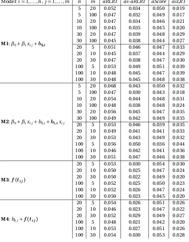
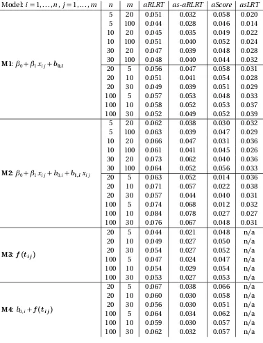
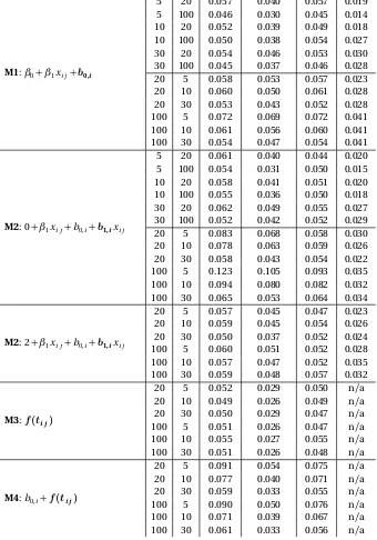
nomi-nalα=0.05 level based on 5000 datasets, by generating model. The bolded term indicates the random effect or smooth function being tested. Legend:n: number of subjects or groups,m: number of obser-vations per subject or group. . . 40 Table 3.2 Empirical type I error rates for testing Bernoulli (binary) responses
at the nominalα=0.05 level based on 5000 datasets, by generating model. The bolded term indicates the random effect or smooth func-tion being tested. Legend:n: number of subjects or groups,m: number of observations per subject or group. . . 41 Table 3.3 Empirical type I error rates for testing Poisson responses at the
nomi-nalα=0.05 level based on 5000 datasets, by generating model. The bolded term indicates the random effect or smooth function being tested. Legend:n: number of subjects or groups,m: number of obser-vations per subject or group. . . 43 Table 4.1 Empirical type I error rates for binary responses using theaRLRT
andaScore methods at the nominalα = 0.05 level based on 5000 datasets, by number of subjects,n, and form of the smooth coefficient,
β(t). Only rejection probabilities corresponding to type I errors are displayed. The maximum standard error was 0.0035. . . 59 Table 4.2 Testing results for the diffusion tensor imaging (DTI) dataset using
Table A.1 Estimated type I error rates for the standard (Tn) and extended (Tn0) bootstraptest statistics with uniform or non-uniform distributed sam-pling points. The nominalα=0.05 and 0.10 levels are based on 5000 simulated datasets forn=100 subjects andm=10 observations per subject. . . 74 Table A.2 Estimated type I error rates for the bootstrap test at the nominal
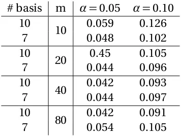
α= 0.05 and 0.10 levels using 10 (default) or 7 basis functions for the alternative model fit in equation (2.6) based on 5000 simulated datasets forn=100 subjects, by number of observations per subject (m). . . 76 Table A.3 Empirical type I error rates for themultivariatetest at the nominalα=
0.05 level based on 5000 datasets, for the asymptotic normal (Z) and weighted chi-squared (ωχ2) distributions, and equally- and unequally-spaced data. . . 79 Table B.1 Empirical type I error rates for testing Binomial responses at the
nom-inalα=0.05 level based on 5000 datasets, by simulating model and number of observations. Bolded terms indicate the random effect or smooth function being tested. Legend:n: number of subjects,mi=m: number of observations per subject. . . 85 Table B.2 Empirical type I error rates for testing binary (Bernoulli) responses
at the nominalα=0.05 level based on 5000 datasets, by simulating model and number of observations. Bolded terms indicate the random effect or smooth function being tested. Legend: # r.effects: number of random effects,n: number of subjects,mi=m: number of groups or observations per subject. . . 88 Table B.3 Empirical type I error rates for testing Poisson responses at the
nom-inalα=0.05 level based on 5000 datasets, by simulating model and number of observations. Bolded terms indicate the random effect or smooth function being tested. Legend:n: number of subjects,mi=m: number of observations per subject. . . 89 Table B.4 Empirical type I error rates for testing Binomial (denominator=8)
Table C.1 Empirical type I error rates for binary data withn =100 subjects at the nominalα=0.05 level based on 5000 datasets using theaRLRT andaScoremethods, by number of observations per subject,m, and form of the smooth coefficient,β(t). Only rejection probabilities cor-responding to type I errors are displayed. The maximum standard error was 0.0035. . . 102 Table C.2 Empirical type I error rates for binary responses using theaRLRT,
aScore,aPFR,FPCR, andaFGAM methods at the nominalα=0.05 level based on 5000 datasets, by number of subjects,n, and form of the smooth coefficient,β(t). Only rejection probabilities corresponding to type I errors are displayed. The maximum standard error was 0.0035.105 Table C.3 Empirical type I error rates for Normal responses at the nominal
α=0.05 level based on 5000 datasets, by number of subjects,n, and form of the smooth coefficient,β(t). Only rejection probabilities cor-responding to type I errors are displayed. The maximum standard error was 0.0035. . . 109 Table C.4 Empirical type I error rates for Binomial (ni=8) responses at the
nom-inalα=0.05 level based on 5000 datasets, by number of subjects,n, and form of the smooth coefficient,β(t). Only rejection probabilities corresponding to type I errors are displayed. The maximum standard error was 0.0035. . . 111 Table C.5 Empirical type I error rates for Poisson responses at the nominal
LIST OF FIGURES
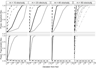
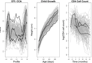
Figure 2.1 Power under the quadratic (top) and trigonometric (bottom) devia-tions from the null, by number of observadevia-tions per subject,m. Shown are:bootstraptest (solid),multivariatetest (long and short-dash), anddirecttest (long-dash), forn=50 (light gray),n =100 (dark gray) andn=500 (black) subjects. Themultivariatetest is not applicable whenm<80. . . 21 Figure 2.2 (left) Diffusion tensor imaging (DTI) of corpus callosum (CCA)
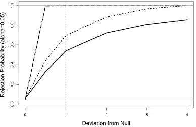
base-line tract profiles from 99 multiple sclerosis patients. (middle) Height measurements (cm) for 215 children from 0 to 729 days after birth. (right) Log-transformed CD4 cell counts from 208 subjects for -18 to 52 months since seroconversion. On each plot, three example trajectories are highlighted in black. . . 23 Figure 2.3 Power for thebootstrap(black) anddirect(gray) tests for data based
on the standard CD4 dataset (solid), dataset with double the number of subjects (short dash), and dataset with double the observations per subject (long dash). The vertical dashed line indicates the effective power of the tests, where data is simulated directly from the estimated alternative covariance (δ=1,r =0). From left to right, the settings for(δ,r)are(0, 0),(0.5, 0),(1, 0),(1, 1),(1, 2),(1, 3). . . 26 Figure 3.1 Power for Bernoulli responses at theα=0.05 level based on 1000
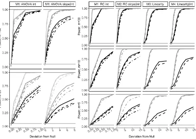
sim-ulated datasets, by simulation model. Legend:aRLRT(solid),aScore (short dash),as-aRLRT(long dash),asLRT (short & long dash). Right plots:n=5 groups (black),n =10 groups (dark gray),n =30 groups (light gray). Left plots:n=20 subjects (black),n =100 subjects (gray). 44 Figure 4.1 Power for dense binary data at theα=0.05 level based on 5000
sim-ulated datasets, byβ(t)form. Legend:aRLRT (black),aScore(gray), n=100 subjects (solid),n=500 subjects (dashed). . . 61 Figure 4.2 (Left) Phoneme curves with two example “aa" (black) and “ao" (white)
highlighted curves. (Right) Estimated coefficient function. . . 62 Figure 4.3 Baseline diffusion tensor imaging tracts for the corpus callosum
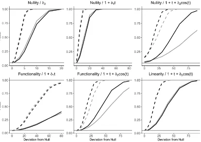
Figure 4.4 (Top left) Exampleβ(t) =δβˆ(t), whereδcontrols magnitude and ˆ
β(t) is the estimated smooth coefficient. Legend:δ = 0 (dotted),
δ=1 (solid),δ=3 (long dash),δ=5 (short dash). (Remaining pan-els) Power for simulated data at theα= 0.05 level based on 5000 simulated datasets for tests for nullity, functionality, and linearity. Legend:aRLRT (black),aScore(gray), standard dataset (solid), data with×2 subjects (dashed). . . 65 Figure A.1 Power for thebootstraptest under the quadratic (top) and
trigonomet-ric (bottom) deviations from the null forn =100 subjects andm=10 observations per subject. Shown are the standardTnstatistic (black, solid) and extendedT0
n statistic (gray, dashed) for the quadratic devia-tion (top) and trigonometric deviadevia-tion (bottom). Note that the x-axis range differs between the quadratic and trigonometric deviations. . 75 Figure A.2 Power for thebootstraptest under the quadratic (top) and
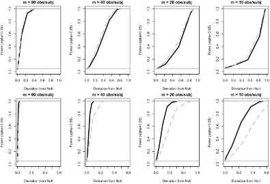
trigono-metric (bottom) deviations from the null, by number of observations per subject (m). Shown are: (default) 10 basis functions (black, solid) and 7 basis function (gray, dashed). Note that the x-axis range differs between the quadratic and trigonometric deviations. . . 77 Figure A.3 Power for themultivariatetest under the quadratic (top) and
trigono-metric (bottom) deviations from the null. Shown are: Equally-spaced (black) and unequally-spaced (gray) timepoints forn=100 (solid) andn = 500 (dashed) subjects. Note that the x-axis range differs between the quadratic and trigonometric deviations. . . 80 Figure B.1 Power for Normal responses at theα=0.05 level based on 1000
simu-lated datasets, by simulation model. Legend:aRLRT (solid),aScore (short dash),as-aRLRT(long dash),asLRT (short & long dash). Right plots:n=5 groups (black),n =10 groups (dark gray),n =30 groups (light gray). Left plots:n=20 subjects (black),n =100 subjects (gray). 82 Figure B.2 Power for Poisson responses at theα=0.05 level based on 1000
sim-ulated datasets, by simulation model. Legend:aRLRT(solid),aScore (short dash),as-aRLRT(long dash),asLRT (short & long dash). Right plots:n=5 groups (black),n =10 groups (dark gray),n =30 groups (light gray). Left plots:n=20 subjects (black),n =100 subjects (gray). 83 Figure B.3 Power for Binomial (denominator= 8) responses at theα = 0.05
Figure B.4 Comparison of power foraRLRT andaRLRT2methods for testing Bernoulli responses withm =5 at theα=0.05 level based on 1000 simulated datasets, by simulation model. Legend:aRLRT (black), aRLRT2(gray),n =20 (solid),n=100 (dashed). . . 91 Figure B.5 Comparison of power for theaRLRT andaRLRT2methods testing
Bernoulli responses withm=10 at theα=0.05 level based on 1000 simulated datasets, by simulation model. Legend:aRLRT (black), aRLRT2(gray),n =20 (solid),n=100 (dashed). . . 92 Figure B.6 Comparison of power for theaRLRT andaRLRT2methods testing
Bernoulli responses withm=30 at theα=0.05 level based on 1000 simulated datasets, by simulation model. Legend:aRLRT (black), aRLRT2(gray),n =20 (solid),n=100 (dashed). . . 93 Figure B.7 Comparison of power for theaRLRT andaRLRT2methods testing
Poisson responses withm =5 at theα=0.05 level based on 1000 simulated datasets, by simulation model. Legend:aRLRT (black), aRLRT2(gray),n =20 (solid),n=100 (dashed). . . 94 Figure B.8 Comparison of power for theaRLRT andaRLRT2methods testing
Poisson responses withm=10 at theα=0.05 level based on 1000 simulated datasets, by simulation model. Legend:aRLRT (black), aRLRT2(gray),n =20 (solid),n=100 (dashed). . . 95 Figure B.9 Comparison of power for theaRLRT andaRLRT2methods testing
Poisson responses withm=30 at theα=0.05 level based on 1000 simulated datasets, by simulation model. Legend:aRLRT (black), aRLRT2(gray),n =20 (solid),n=100 (dashed). . . 96 Figure B.10 Comparison of power for theaRLRT andaRLRT2methods testing
Binomial responses withm =5 at theα=0.05 level based on 1000 simulated datasets, by simulation model. Legend:aRLRT (black), aRLRT2(gray),n=20 (solid),n =100 (dashed). . . 97 Figure B.11 Comparison of power for theaRLRT andaRLRT2methods testing
Binomial responses withm =10 at theα=0.05 level based on 1000 simulated datasets, by simulation model. Legend:aRLRT (black), aRLRT2(gray),n =20 (solid),n=100 (dashed). . . 98 Figure B.12 Comparison of power for theaRLRT andaRLRT2methods testing
Binomial responses withm =30 at theα=0.05 level based on 1000 simulated datasets, by simulation model. Legend:aRLRT (black), aRLRT2(gray),n =20 (solid),n=100 (dashed). . . 99 Figure C.1 Power for theaRLRT method for binary data withn=100 subjects at
theα=0.05 level based on 5000 simulated datasets. Legend:m=80 (black),m =40 (blue),m=20 (green),m=10 (red), estimated curve error (σ2X =σˆ2
X, solid),×1000 curve error (σ
2
X =1000 ˆσ
2
Figure C.2 Power for theaScoremethod for binary data withn=100 subjects at theα=0.05 level based on 5000 simulated datasets. Legend:m=80 (black),m =40 (blue),m=20 (green),m=10 (red), estimated curve error (σ2X =σˆ2
X, solid),×1000 curve error (σ
2
X =1000 ˆσ
2
X, dashed). . . 104 Figure C.3 Power for binary data at theα=0.05 level based on 5000 simulated
datasets, byβ(t)form. Legend:aRLRT(black),aScore(gray),aPFR (blue),FPCR(green; not valid forn=100),aFGAM(red),aFtest (or-ange; not valid for Bernoulli),n=100 subjects (solid),n=500 sub-jects (dashed). . . 106 Figure C.4 Power for Normal data at theα=0.05 level based on 5000 simulated
datasets, byβ(t)form. Legend:aRLRT(black),aScore(gray),aPFR (blue),FPCR(green, not valid forn =100),aFGAM(red),aFtest,n= 100 subjects (solid),n=500 subjects (dashed). . . 108 Figure C.5 Power for Binomial data (ni=8 draws) at theα=0.05 level based on
5000 simulated datasets, byβ(t)form. Legend:aRLRT(black),aScore (gray),aPFR(blue),FPCR(green),aFGAM (red),aFtest(orange; not valid forn =100),n=100 subjects (solid),n=500 subjects (dashed). 110 Figure C.6 Power for Poisson data at theα = 0.05 level based on 5000
CHAPTER
1
INTRODUCTION
1.1
Functional Data
Functional data consists of continuous and infinite-dimensional curves or data observed over a continuum rather than a single fixed point. For example, an individual child’s height can be considered to be a function of their age. That is, while height measurements may be made yearly at annual checkups, height can reasonably be assumed to change continuously and smoothing with age. Functional data analysis (FDA) is a branch of statistics focused on visualizing, modeling, and analyzing functional data; see Ramsay and Silverman (2002) for an overview. While many common analysis tools build on or extend existing methods for univariate and multivariate data, functional data presents unique opportunities and challenges.
Consider a set of functional observations{(Yi j,ti j):i =1, . . . ,n;j =1, . . .mi}, whereYi j is a scalar response observed at theit hsubject’s jt h point,t
noise,εi j. That is
Yi j=Xi(ti j) +εi j (1.1)
whereXi(·)are square-integrable random processes inL2(T )with unknown smooth mean and covariance functions,µ(t)andG(t,t0), respectively, andε
i j is white noise with zero mean and varianceσ2. For simplicity,X
i(·)are typically assumed to be independent and identically distributed (iid) that are independent ofεi j. Most importantly,Xi(·)is assumed to be ordered and smooth, that is, the relationship betweenXi(t)andXi(t0)depends on (a) ift <t0ort >t0and (b) how close the values oft andt0are. This ensures thatXi(·)is differentiable and that values observed within a short neighborhood oft are correlated (Ramsay and Silverman, 2002). These assumptions separate functional data methods from longitudinal or multivariate data techniques.
Functional data may be observed at a set of (a) dense or (b) sparse observation points. For dense data, observations are made at the same points for all subjects and are often made on a high-frequency grid of equally spaced points. This design is comparable to high-frequency multivariate data. For sparse data, observation points differ across subjects and often occur at a few spaced points. This design is comparable to randomly-observed longitudinal data.
1.2
Outline and Contributions
In Chapter 2, we propose a goodness-of-fit test for comparing a parametric covariance function against a general nonparametric alternative in the context of sparse and dense functional data. We illustrate the utility of this method by testing the fit of a quadratic polynomial covariance, that is, comparing a linear mixed effects model against a functional data alternative, such as the child growth example outlined in Chapter 1.1. We propose a distance-based test statistic that compares the covariances estimated under the null and alternative hypothesis. The null covariance is estimated directly from the null model, in this case a linear mixed effects models, and the alternative covariance is estimated using functional principal components. The null distribution of the test statistic is then obtained using a wild bootstrap algorithm that generates samples using the estimated null covariance and residuals under the alternative hypothesis. We demonstrate the efficacy of our method with a simulation study and application to diffusion tensor imaging, child growth, and CD4 cell counts for HIV+patients.
In Chapter 3, we propose an approximate restricted likelihood ratio test for random effects (zero-value variance components) in generalized linear mixed models (GLMMs). We motivate this method using a study of salamander mating behavior, where random effects represent individual male or female behavior. Determining the significance of individual behavior can be done by testing these random effects. This method is also applicable to functional data where it can be used to test nonparametric regression models. In this scenario, the nonparametric (functional) model can be represented as a mixed model using penalized splines, allowing for testing of the functional form by testing random effects. Our method extends the penalized quasi-likelihood approach for estimating GLMMs to conduct testing directly on the “normalized" working responses and linear mixed model used for estimation. This allows for the test statistic and its null distribution to be approximated using results for normal responses. We show in a simulation study that our method has better performance compared to several competitors. We develop and publish an
R
package to implementing this approach.(non-functional) and functional logistic regression models, and find that the functional model has better predictive power. This observation can be formally analyzed by testing the functional form of the predictor. Thus, we develop a flexible mixed model representation for the scalar-on-function linear model that presents testing in terms of single random effect. We then apply the approximate restricted likelihood ratio test from Chapter 3 to conduct hypothesis testing. We also consider extensions of several existing methods, and show through a simulation study that our method has better performance.
The remainder of this chapter provides an overview of select topics in statistics and functional data analysis utilized in subsequent chapters.
1.3
Smoothing
As discussed for equation (1.1), functional data is assumed to be a realization of an un-derlying smooth process, but is frequently observed with noise or measurement error. Smoothing is a technique for processing these noisy observations to “smooth out" noise and identify the true underlying function. The standard approach for smoothing uses a linear combination ofk=1, . . . ,K basis functions,Bk(t), to represent the underlying func-tion. Typical bases used include Fourier basis, polynomial splines, and wavelets, and the choice of bases should depend on the application (Ramsay and Silverman, 2005). We can represent our smooth function,Xi(t), as
Xi(t) =µ(t) + K X
k=1
gkBk(t), (1.2)
wheregk is the basis coefficient for thekt hbasis function. This parameter,K, controls the dimensionality of the basis representation and is typically chosen using cross-validation or AIC; see Wood (2003) for discussion.
chapters.
Estimating the spline basis can be done using least squares by minimizing the criterion SS E =Pni=1Pmij=1[Yi j−
Pk
k=1gkBk(ti j)]2. This criterion can be modified to account for cor-related errors using weighted lease squares, or to impose additional smoothness by adding a roughness penalty; see Ramsay and Silverman (2005) for discussion.
1.4
Functional Principal Components Analysis
Functional principal components analysis (FPCA) is a common technique for exploring and representing functional data. FPCA extends the standard principal components anal-ysis method for multivariate data by accounting for high-frequency of observations and potential sparsity of observed data. This section will briefly describe FPCA for dense or sparse functional data.
Using Mercer’s theorem, we can represent the covariance of Xi(t)with the spectral decompositionG(t,t0) =P∞
k=1λkφk(t)φk(t), whereλk is thek
t hordered eigenvalue cor-responding to orthonormal eigenfunctionφk. We can then use a Karhunen-Loéve (KL) expansion to representXi(t)as
Xi(t) =
∞
X
k=1
ξi kφk(t), (1.3)
whereξi k =R
T[Xi(t)−µ(t)]φk(t)d tis thei
t hsubject’s score for thekt heigenfunction. These score coefficients are typically assumed to be independent acrossi with zero mean and varianceλk. In practice, both the spectral decomposition and KL-expansion are truncated to a finite number of eigenfunctions,K, such thatG(t,t0)≈PK
k=1λkφk(t)φk(t)andXi(t)≈
PK
k=1ξi kφk(t). This truncation allows for dimension reduction of the observed functional
process and helps remove noise from the predicted covariance and individual functions. The truncation parameter,K, can be chosen using a minimum percent variance explained (PVE) or AIC (Yao et al., 2005; Xiao et al., 2016; Li et al., 2013).
Estimating the spectral decomposition and KL-expansion differs depending on sam-pling frequency. For dense data, where all subjects are observed at the same points, estima-tion can be done directly from the sample covariance ˆG(ti j,ti j0) =n1−1
Pn
i=1[Yi j−µˆ(ti j)][Yi j0−
ˆ
µ(ti j0)], where ˆµ(t)is the estimated mean function. The observed data is often noisy, so
and Ramsay, 1986; Staniswallis and Lee, 1998; Yao et al., 2005; Xiao et al., 2016). The spec-tral decomposition can then be calculated from the smoothed covariance and the scores computed using numerical integration or the best linear unbiased predictors (BLUPs) (Yao et al., 2005; Xiao et al., 2016).
FPCA for sparse data, where subjects are observed at different points, is more challeng-ing and typically follows one of two approaches: (a) smooth and diagonalize the sample covariance (Yao et al., 2005; Xiao et al., 2018) or (b) estimate the basis functions from smoothed sample curves to reconstruct a reduced rank covariance approximation (James et al., 2000; Peng and Paul, 2009). The former approach is generally more efficient and pop-ular. Again, the spectral decomposition can be calculated from the smoothed covariance the scores computed using BLUPs (Yao et al., 2005; Xiao et al., 2018).
1.5
Hypothesis Testing
The goal of hypothesis testing is to compare evidence between null and alternative hy-potheses,H0andHA, respectively, that present complementary statements about the true
underlying population (Casella and Berger, 2002). For example, in the child height applica-tion described in Secapplica-tion 1.1, we may be interested in comparing hypotheses about the rate of individual growth. Our default or null hypothesis may be that growth is linear over time, versus an alternative hypothesis that growth is non-linear. That is,H0:Xi(t) =b0,i+b1,it versusHA:Xi(t)6=b0,i+b1,it, whereb0,i is theit hchild’s intercept (height at age 0) andb1,i is their rate of growth. This example is considered more formally in Chapter 2.
We can compare these hypotheses using a hypothesis test, which specifies for what sample values the decision is made to either (a) acceptH0as true or (b) rejectH0and accept
HAas true (Casella and Berger, 2002). These tests typically consist of a test statistic, some function of the observed sample, and a cutoff value or rejection region for that statistic. Standard tests include score, Wald, likelihood-ratio (LRT), and F-tests, which are defined by a scalar test statistic and a cutoff value based on the distribution of the statistic under the null hypothesis. We will briefly review the LRT and restricted-likelihood ratio test (RLRT) to be used in later chapters.
The LRT for hypothesesH0:θ ∈Θ0versusHA:θ ∈ΘAhas the form
L RT =supΘ0L(θ|x)
whereL(θ|x)is the likelihood for observed datax= (x1, . . . ,xn)T evaluated at valueθ and cutoff point,c, for rejectingH0. The RLRT has the same form as equation (1.4) but replaces
L()withR E L(), the restricted likelihood. The restricted likelihood transforms the data so that nuisance parameters do not affect estimation of the parameters of interest, which improves estimation accuracy for variance components (Pinheiro and Bates, 2000).
The cutoff value,c, is determined by the significance level, or maximum type I error rate (probability of rejectingH0whenH0is true) and the distribution of the statistic under the
null hypothesis. If the true parameter value is not on the boundary of the parameter space, then from Wilk’s theorem, the LRT and RLRT have an asymptotic chi-squared distribution with degrees of freedom (d f) equal to the difference in number of parameters for the null and alternative hypotheses. Thus, the cutoff value for aα-level test would beχ2
1−α,d f. When the true value lies on parameter space boundary, as when testing zero-value variance com-ponents, the asymptotic null distribution is instead a mixture of chi-square distributions based on the number of fixed effects being tested (Self and Liang, 1987; Stram and Lee, 1994). However, this asymptotic result assumes that data can be divided into independent and identically distributed (iid) subvectors tending to infinity. These assumptions are often violated for mixed model representations for functional data, leading to conservative tests (Pinheiro and Bates, 2000; Scheipl et al., 2008). Crainiceanu and Ruppert (2004) describe the finite-sample distribution for Gaussian responses under this setting, which improves both the power and type I error of the test. Chapter 3 considers the RLRT for testing variance components with generalized responses.
CHAPTER
2
A SMOOTHING-BASED
GOODNESS-OF-FIT TEST OF
COVARIANCE FOR FUNCTIONAL DATA
2.1
Introduction
1Functional data have become increasingly common in fields such as medicine, agriculture,
and economics. Functional data usually consist of high frequency observations collected at regular intervals, see Ramsay and Silverman (2002) and Ramsay and Silverman (2005) for an overview of methods and applications. By comparison, longitudinal data typically consist of repeated observations collected at a few time points varying across subjects. In recent years, functional data methods have been successfully extended and applied to longitudinal data (James et al., 2000; Yao et al., 2005). While these methods are more flexible, 1This chapter is joint work with Luo Xiao and Ana-Maria Staicu, and will appear in an upcoming volume
their estimation and interpretation are more cumbersome than longitudinal methods and require more sampling units or observations for accurate and reliable estimates. Thus, it is natural to question if such flexibility is truly necessary. This paper focuses on comparing longitudinal data methods with functional data methods. For example, we consider the case of testing if a simple linear mixed effects model is sufficient for longitudinal data or if a more complex functional data model is required.
This work is motivated by the CD4 cell count dataset from the Multicenter AIDS Cohort Study (Kaslow et al., 1987). CD4 count is a key indicator for AIDS disease progression, and understanding its behavior over time is critical for monitoring HIV+patients. The dataset is highly sparse, with 5 to 11 irregularly-spaced observations per subject. CD4 counts have been extensively analyzed using longitudinal data methods, e.g., semiparametric and linear random effects models (Taylor et al., 1994; Zeger and Diggle, 1994; Fan and Zhang, 2000). Recently, functional data methods have also been applied to this data (Yao et al., 2005; Goldsmith and Crainiceanu, 2013; Xiao et al., 2018). While the nonparametric functional data methods are highly flexible and better adapt to subject-specific patterns, they are more difficult to implement and interpret compared to the parametric approaches. Therefore it is of interest to test whether the simpler longitudinal methods are sufficient for the data. To the authors’ best knowledge, no formal testing procedure exists for this application.
The inherent difference between functional and traditional longitudinal data methods is in the correlation model between repeated observations. For functional methods, the covariance within a subject is assumed to be smooth with an unknown nonparametric form. The covariance can be estimated by smoothing the sample covariance (Besse and Ramsay, 1986; Yao et al., 2005; Xiao et al., 2018) or constructing a reduced rank approximation by estimating basis functions from smoothed sample curves (James et al., 2000; Peng and Paul, 2009). In contrast, longitudinal data approaches typically assume a simple parametric covariance structure with a few parameters, such as autoregressive or exponential (see Diggle et al. (2002) for an overview), or induced by a random effects model (Laird and Ware, 1982).
a “wild" bootstrap algorithm for finite samples. Comparisons have also been applied to functional regression for model diagnostics and evaluating assumptions (Chiou and Müller, 2007; Bücher et al., 2011) and testing functional coefficients (Swihart et al., 2014; McLean et al., 2015; Kong et al., 2016). The proposed method is an extension of smoothing-based methods to test the form of the covariance function.
For high-dimensional multivariate data, where observation points are regular and balanced (same for all subjects), a number of methods exist to test an identity or spherical covariance matrix against an unstructured alternative (Ledoit and Wolf, 2002; Bai et al., 2009). Recently, Zhong et al. (2017) develop a general goodness-of-fit test that can be applied to many common parametric covariances. However, these methods are ill-suited for the comparison between functional and longitudinal data models because they (a) fail to account for the underlying smoothness of the process and (b) require data observed at fixed time points for all subjects, i.e., a (fixed) common designThe CD4 dataset has an irregular design where time points differ for each subject, so cannot be tested with these approaches. Note that therandom design, where observed time points are independent between and within the subjects, is a special case of the irregular design. Common or random designs are typically assumed in theoretical studies of functional data (Cai and Yuan, 2011).
The objective of this paper is to develop a testing procedure for comparing parametric longitudinal versus nonparametric functional data covariance models applied to repeated measured data with irregular and/or highly frequent sampling design. Note that longitudi-nal data with only a few repeated measurements per subject with a regular sampling design is not within the scope of this paper. Selecting an adequate covariance model is critical, because model misspecification can bias estimation and inference, while an unnecessarily complex model can slow computation and interfere with model interpretation. We pro-pose a goodness-of-fit test based on the difference between the estimated parametric and nonparametric covariances, inspired by Hardle and Mammen (1993). Compared to Zhong et al. (2017) for high-dimensional multivariate data, our test statistic can be evaluated using a more flexible modeling approach that accounts for general designs and exploits the underlying smoothness of repeated observations. However, deriving the distribution of the test statistic is challenging and we use bootstrapping to approximate the null distribution. To demonstrate performance and versatility of the proposed test, we present a simulation study and three data applications.
model and hypothesis test, Section 2.3 details the proposed test, and Section 2.4 describes our implementation. Section 2.5 outlines extensions to general smooth covariance func-tions. Section 2.6 presents a simulation study. Section 2.7 details three applications to diffusion tensor imaging, child growth, and CD4 cell count. Finally, Section 2.8 summarizes the paper and discusses limitations of the proposed test and Section 2.9 outlines the online supplementary materials.
2.2
Statistical Framework
Consider functional or longitudinal data{(ti j,Yi j)∈ T ×R:i =1, . . . ,n,j =1, . . . ,mi}wherei denotes the subject index, j denotes the visit index, andYi jis the measurement for thei-th subject at timeti j. Here,n is the number of subjects andmi the number of observations for thei-th subject, which can vary across subjects. Assume thatT = [a,b]is a closed and compact domain. Data are often observed with noise, so we posit the model
Yi j=µ(ti j) +Xi(ti j) +εi j. (2.1)
Hereµ(t)is a smooth mean function,Xi is a zero-mean Gaussian random function in-dependent between subjects, andεi j is Gaussian white noise independently and iden-tically distributed with zero mean and variance σ2, independent of Xi. Let G(t,t0) =
C o v{Xi(t),Xi(t0)}be the covariance function ofXi. Assume thatG is a smooth, positive semidefinite bivariate function defined onT2.
We are interested in the form of the covariance, and would like to test the hypothesis thatG has a known parametric form against a general alternative. Motivated by the CD4 dataset, which has previously been fit with a linear random intercept and slope model, we focus on the quadratic polynomial function
G0(t,t0) =σ02+σ01(t +t0) +σ21t t0, (2.2)
where (σ2
0,σ01,σ 2
1) are unknown parameters. Because this covariance is induced by the
linear random effects modelXi(t) =b0i+b1it, wherebi= (b0i,b1i)T are random effects with
zero mean andV a r(bi0) =σ02,V a r(bi1) =σ21, andC o v(bi0,bi1) =σ01, testingG0is
equiva-lent to testing if a linear random (or mixed) effects model is sufficient for the data. Note that this is a specific case of the general linear random effects modelXi(t) =
PK
for random effectsbi k with zero mean and varianceσ2k and known functionsφk(t), which has covariance functionG0(t,t0) =PK
k=1σ 2
kφk(t)φk(t0) +2 P
k<k0σk k0φk(t)φk0(t0), where
σk k0 =C o v(bi k,bi k0). While we focus on equation (2.2), the proposed test can be easily
adapted for the more general random effects case or any smooth parametric covariance with finite parameters, as discussed in Section 2.5. Ideally, scientific or expert knowledge about the underlying process should guide the choice ofG0. If such information is unavailable, a
commonly used and interpretable structure would be preferred. Formally, the hypothesis test can be written as
H0:G(t,t0) =G0(t,t0)versusHA:G(t,t0)6=G0(t,t0). (2.3)
Under the null hypothesis, the covariance has a specific parametric form with finite pa-rameters. Under the alternative hypothesis, the covariance function is assumed only to be smooth and positive semidefinite. This flexibility may better capture heterogeneity across subjects but is hard to estimate and interpret compared to a parametric model. Therefore, it is desirable to test goodness-of-fit for these two types of models. In the following section, we propose a distance-based goodness-of-fit test for equation (2.3) that can be applied to functional data with either a dense common or sparse irregular sampling design.
2.3
Smoothing-based Test
2.3.1
Null Model
Under the null hypothesis,G =G0is a quadratic polynomial covariance, corresponding to
Xi(t) =b0i+b1it
(bi0,b1i)T ∼N
0,V0=
σ2 0 σ01
σ01 σ12
.
(2.4)
Here,Xi(t)is a linear random effects model with subject-specific random intercepts and slopes,b0i andb1i, respectively. LetYeibe themi-length vector of de-meaned observations for thei-th subject observed at timesti= (ti1, . . . ,ti mi)T, andVi= [1,ti]V0[1,ti]T+σ2Imi be the corresponding covariance matrix, where1is ami-length vector of ones andImi is ami×mi identity matrix. Then the unknown parameters in model (4) can be estimated by maximizing the log-likelihood`(V0,σ2|Yei,ti) =
Pn i=1−
1
2(log|Vi|+YeiTVi−1Yei), where|Vi| is the determinant of the matrixVi, using an expectation-maximization (EM) or Newton-Raphson algorithm, as outlined in Lindstrom and Bates (1988).
2.3.2
Alternative Model
Under the alternative hypothesis, the covariance function has a smooth, nonparametric form. ApproximateGAby smoothing the sample covariance using tensor product regression splines as G(t,t0) =PH
h,`=1θh`Bh(t)B`(t0), where {Bh(t) :h = 1, 2, . . . ,H} are a sequence of cubic B-spline basis functions defined overT andθbh` are coefficients estimated by minimizing the least squares expression
n X
i=1
X
1≤j6=j0≤mi ¨
e Yi jYi je 0−
H X
h,`=1
θh`Bh(ti j)B`(ti j0) «2
, (2.5)
under the natural symmetry constraint thatθh`=θ`h. Denote the estimated alternative covariance asGÒA(t,t0) =
PH
h,`=1θbh`Bh(t)B`(t0).
The measurement error,σ2, in equation (2.1) can be estimated following Yao et al. (2005)
2.3.3
Test Statistic
Using the estimated null and alternative covariances,GÒ0andGÒA, the proposed test statistic is the Hilbert-Schmidt norm distance
Tn=||GÒA− KGÒ0||H S, (2.6)
where||f||H S= qR R
f(t,t0)2d t d t0for bivariate functionf andKGÒ0is the smoothed null covariance estimate using tensor-product B-splines. That is, replaceYei jYei j0withGÒ0(ti j,ti j0)
in the least squares expression in equation (2.5) to estimateθ0,h l =θ0,l h soKGÒ0(t,t0) = PH
h,`=1θb0,h lBh(t)B`(t0). Using the smoothed null eliminates the bias from nonparametric function estimation and is common practice for nonparametric regression tests; see, e.g., Hardle and Mammen (1993). A large Tn indicates that the null parametric covariance approximates the true covariance poorly. The null distribution ofTn is difficult to derive as estimation of the alternative is based on second moments of the observed responses. Moreover, even in settings where the null distribution of distance-based test statistic is available, Hardle and Mammen (1993) show that the test statistic converges slowly and recommends bootstrapping instead. In the next section, we propose a wild bootstrap algorithm (Wu, 1986) for the null distribution ofTn following Hardle and Mammen (1993). Note that one may also consider an empirical version of the proposed test statistic evaluated at the paired time points (see Appendix A.1 for an example); we focus on the form in equation (2.6) throughout this paper.
2.3.4
Approximate Null Distribution of
T
nvia a Wild Bootstrap
Denote thel-th bootstrap sample as{Yi j(l):i =1, . . . ,n,j =1, . . . ,mi,ti j ∈ T }, whereYi j(l)= b
µ(ti j) +Xi(l)(ti j) +εi j(l) for the original time pointsti j. Let µb(t)be the estimated smooth mean function,Xi(l)(ti j)be subject trajectories generated from the estimated null model in equation (2.4), andε(i jl)be simulated residuals using the estimated measurement error in Section 2.3.2. The test statistic,T(l)
n , can be calculated from the resulting bootstrap sample, and the process is repeated to obtain an approximation of the null distribution ofTn. If the observed statistic is large compared to the null approximation, then rejectH0. This “wild"
Algorithm 1Parametric Bootstrap for Null Distribution ofTn
1: for l ∈ {1, . . . ,L}do
2: GenerateXi(l)(ti j) =b0(il)+b1(li)ti j from(bi(0l),b1(il))T ∼N(0, Ò
V0)fori ∈ {1, . . . ,n}, where
Ò
V0is the estimated parameter matrix under the null hypothesis in (4).
3: Sampleε(i jl)∼N(0, ˆσ2)fori∈ {1, . . . ,n}and j ∈ {1, . . . ,mi}, where ˆσ2is the
measure-ment error estimated under the alternative model in Section 2.3.2.
4: Define thel-th bootstrap dataset asYi j(l)=µb(ti j) +X
(l)
i (ti j) +ε( l) i j.
5: Estimate and subtract the mean function for the bootstrap data,µ(l)(t).
6: Fit thel-th bootstrap dataset with model (2.4) and estimateGÒ( l)
0 .
7: Fit thel-th bootstrap dataset with model (2.5) and calculateGÒ( l) A .
8: Calculate the test statisticT(l) n =||GÒ(
l)
A − KGÒ( l)
0 ||H S.
9: end for
10: Calculatep-value=L−1PL l=1I(T(
l)
n >Tn), whereIis an indicator function with value 1 if the condition is true, and 0 otherwise.
2.4
Implementation
First, estimate the smooth meanµ(t)using thin plate regression splines (Wood, 2003) using the
gam
function in theR
packagemgcv
(Wood, 2018), and subtract from the data. The null model in equation (2.4) is a standard random effects model that can be estimated using thelme
function in theR
packagenlme
(Pinheiro et al., 2018). For the least squares expression in (5) to smooth the alternative and null covariance estimates, we useH =10 cubic B-splines per axis with equally-spaced interior knots. The choice of 10 B-B-splines balances performance and computational speed, see Appendix A.2 for a sensitivity study. While the number of splines needs only be sufficiently large, additional splines may be needed if the data is known or observed to be highly wiggly. Cross-validation or Aikaike information criterion (AIC) may be used for a formal selection (see Wood (2003) for discussion).2.5
Extensions
2.5.1
Smooth Covariance
Any smooth parametric covariance function can be tested using the proposed procedure, with modification to the null model and bootstrap algorithm. For example, consider the stationary Gaussian or quadratic exponential covariance functionG0(t,t0) =θe−h2/δ2
h=|t−t0|, and (θ,δ) are parameters to be estimated. The null model can be estimated using likelihood-based methods, and bootstrap data generated asYi(l)=µˆi+VÒ
(l)1 2
0i z+
(l)
i , where ˆ
µiis the estimated mean vector of lengthmi,VÒ( l)
0i is the estimated null covariance matrix defined by(θb,δb),X
1
2 is the square root matrix whereX 1 2X
1
2 =X,zis anm
i-length vector of independent samples from a standard normal distribution, and(il)is an independent vector of residuals fromN(0, ˆσ2).
2.6
Simulation Study
We conduct a simulation study to evaluate performance of the proposedbootstraptest and two competing methods, described in Section 2.6.1, for testing the hypothesis in equation (2.3) that the covariance has a quadratic polynomial form. Data are generated as
Yi j =µ(ti j) +Xi(ti j) +εi j Xi(ti j) =b0i+b1iti j+∆zi(ti j),
(2.7)
fori =1, . . . ,n subjects and j =1, . . . ,mi observations per subject. The scalar,∆, controls the magnitude of deviation from the null model. The mean,µ(t), is set to 0 and the resid-uals are distributedεi j ∼N(0, 1), independent ofXi. Random intercepts and slopes are sampled from a bivariate normal distribution with zero mean,V a r(bi0) =V a r(bi1) =1 and
C o v(bi0,bi1) =−0.5, independent of the non-linear functionzi, defined below. Theti j are
observed on a grid of 80 equally spaced points in[−1, 1]. Ifmi=80, the subject is observed at all points and ifmi<80, observed time points are uniformly sampled for each subject from the 80 possible points. Tuning parameters are selected as described in Section 2.4. Consider a factorial combination of the following factors:
1. Observations per subject(mi=m): (a)m=80, (b)m=40, (c)m=20, (d)m=10
2. Deviation from the null model:
(a) Quadratic:zi(t) =b2it2,b2i∼N(0, 1) (b) Trigonometric:zi(t) =
P2
k=1ξi kψk(t),
{ψ1(t),ψ2(t)}={sin(2πt), sin(4πt)},ξi k ∼N(0,λk),λ1=λ2=1.
evaluated in terms of the empirical type I error rate (size) for nominal levelsα = 0.05 and 0.10 based on 5000 simulated datasets, and power at theα = 0.05 level with 1000 simulated datasets. Results are presented in terms of deviation from the null, defined as ∆2R
V a r{zi(t)}/V a r{Xi(t)}d t.
2.6.1
Competing Methods
As discussed in Section 2.1, we are unaware of any existing methods for testing covariance that can be applied to all functional or longitudinal data settings. In this subsection, we describe two testing methods that can be applied to specific scenarios of the hypothesis test in equation (2.3).
2.6.1.1 Direct Test
Consider the case where covariance under the alternative hypothesis has a known, para-metric form so the null model forXiis nested within the alternative model. In essence, test if a more complex covariance better explains the data than the null covariance. For the quadratic polynomial covariance, an alternative may beGA(t,t0) =σ2
0+σ01(t+t0)+σ 2 1t t0+
σ2 2t
2t02. Then the alternative model can be written as
Xi(ti j) =b0i+b1iti j+b2iti j2
bi= (b0i,b1i,b2i)T ∼N
0,
σ2
0 σ01 0
σ01 σ12 0
0 0 σ2
2 . (2.8)
Note that this is the model for the quadratic deviation setting in the simulation study. Like the null model, equation (2.8) can be estimated using the
lme
function in theR
packagenlme
(Pinheiro et al., 2018). The hypothesis test is equivalent to testing ifb2i=0, orH0:G(t,t0) =G
0(t,t0)⇔σ22=0 versusHA:G(t,t0)6=G0(t,t0)⇔σ22>0.
pseudolikeli-hood. Because of the limited sample size in our simulation study, we use the finite sample null distribution from Greven et al. (2008), which can be preformed efficiently using the
exactRLRT
function in theR
packageRLRsim
(Scheipl and Bolkner, 2016).2.6.1.2 Multivariate Test
The Zhong et al. (2017) test for high-dimensional multivariate data can be applied to functional data with a common design. Consider a repeated measures modelYi=µ+i,
whereYi = (Yi1, . . . ,Yi m)T is a vector of responses,µis a mean vector of lengthm, and residuals are distributedi ∼ N(0,G). Denoteθ0 as the parameter vector defining the covariance matrix under the null hypothesis,G0. LetGAbe the alternative unstructured covariance.
Based on the squared-Frobenius distance between the null and alternative covariances,
δ(θ0) =t r(GA−G0)2, Zhong et al. (2017) propose the test statisticΛn=TnÒ−Jnb3, whereTnÒ is an unbiased estimator forδ(θ0)and Jnb adjusts for errors in the estimation ofθ0. The
hypothesis test in equation (2.3) can be conducted by testing ifΛn is significantly larger than 0. With some assumptions on the covariance structure, the asymptotic normal and fixed sample weighted-chi square null distributions can be determined for any parametric covariance, and we provide derivations for the quadratic polynomial covariance in Appendix A.3. In our simulation study, themultivariatetest can only be applied to the densem=80 case, and we use 10,000 samples to approximate the fixed sample null distribution. In Appendix A.4, we also consider performance of themultivariatetest in less-ideal settings with smallm and unequally-spaced data.
2.6.1.3 Limitations of the Competing Methods
Table 2.1Estimated type I error rates for thebootstrap,direct, andmultivariatetests at the nomi-nalα=0.05 and 0.10 levels based on 5000 datasets, by number of subjects (n) and observations per subject (m). The standard error was 0.003 and 0.004 forα=0.05 andα=0.01, respectively. Themultivariatetest is applicable for only the densem=80 setting.
bootstrap direct multivariate
n m α=0.05 α=0.10 α=0.05 α=0.10 α=0.05 α=0.10
100
10 0.059 0.126 0.044 0.086 n/a n/a
20 0.045 0.105 0.049 0.098 n/a n/a
40 0.042 0.093 0.049 0.102 n/a n/a
80 0.042 0.091 0.045 0.096 0.053 0.103
500
10 0.047 0.105 0.049 0.096 n/a n/a
20 0.050 0.103 0.049 0.096 n/a n/a
40 0.050 0.100 0.043 0.090 n/a n/a
80 0.044 0.093 0.046 0.096 0.053 0.105
2.6.2
Simulation Results
Table 2.1 reports the empirical type I error rates for all three methods. As themultivariate test requires a common sampling design, it can only be applied to them=80 setting. We report only the fixed-sample weighted chi-squared distribution; results for the asymptotic normal distribution were similar and are presented in Appendix A.4. All three methods have empirical levels close to the nominal levels, although both thebootstrapanddirect tests can be slightly conservative for several settings.
Figure 2.1Power under the quadratic (top) and trigonometric (bottom) deviations from the null, by number of observations per subject,m. Shown are:bootstraptest (solid),multivariatetest (long and short-dash), anddirecttest (long-dash), forn=50 (light gray),n=100 (dark gray) and
n=500 (black) subjects. Themultivariatetest is not applicable whenm<80.
dataset is small and deviation from the null is small. For example, whenn=100 andm =10, the test is underpowered for the quadratic deviation when signal size is small.
2.7
Applications
2.7.1
Diffusion Tensor Imaging
We first consider a dataset of diffusion tensor imaging (DTI) of intracranial white matter microstructure with dense, common sampling design for a group of normal and multiple sclerosis patients. Images of the white matter are depicted with tract profiles shown in Figure 2.2 and available in the
R
packagerefund
(Goldsmith et al., 2018); see Reich et al. (2010) for study details. Goldsmith et al. (2011) consider this dataset for modeling multiple sclerosis disease status, concluding that inclusion of the tract profile as a functional pre-dictor improves model performance compared to a subject-specific average of the profile. Note that a subject-specific average is equivalent to the subject-specific intercept in the null model in (2.4). We evaluate this conclusion formally by testing if a quadratic polynomial covariance is sufficient for modeling the tract profiles, using thebootstrap,multivariate, anddirecttests.We focus on the baseline tract profiles of the corpus callosum (CCA), associated with cognitive function, for multiple sclerosis patients, observed on a dense, regular grid of 93 points. After removing subjects with missing observations, the dataset has profiles from 99 subjects, for a total of 9207 observations. Tuning parameters are selected as described in Section 2.4. The observed test statistic for thebootstraptest isTn=0.071 corresponding to p<0.001. Thedirecttest yields an RLRT statistic of 1160.6 corresponding top<1×10⁻¹⁶.
The multivariate test yields an observed test statistic of Λn = 0.058, corresponding to p<0.001 for both the weighted chi-squared and asymptotic normal distributions. All three tests support the conclusion that a quadratic polynomial covariance is inadequate for the data, and that a functional method should be used.
2.7.2
Child Growth Measurements
for the data. We consider this observation formally by testing the quadratic polynomial covariance for the growth data using thebootstrapanddirect tests.
The observed test statistic for thebootstraptest isTn=494.13, corresponding top = 0.031, while the RLRT statistic from thedirect test is 2205.8, corresponding top <0.001. Both tests indicate that the parametric quadratic polynomial covariance is not sufficient for the data, and a functional approach should be used instead.
2.7.3
CD4 Count Data
Last, we consider the motivating example of CD4 cell counts described in Section 2.1 by conducting a formal test of the quadratic polynomial covariance using thebootstrapand directtests. The dataset is available in the
R
packagerefund
(Goldsmith et al., 2018) and includes cell counts from -18 to 52 months since seroconversion; we log-transform the counts to stabilize variability. We consider only subjects with at least 5 observations and who have log-transformed cell counts greater than 4, for a total of 1402 observations from 208 subjects (5-11 observations per subject). The cleaned and log-transformed data are shown in Figure 2.2.Because data are sparser than the settings considered in the full study, we conduct a small simulation study to check the size and power of the tests. Simulated data are generated asYi j =Xi(ti j) +εi j, whereXi(ti j)is defined below,ti j are the time points in the original dataset, andεi j ∼N(0, ˆσ2), where ˆσ2is the estimated error variance under the alternative model. The random functionXi(t)is generated from a multivariate normal distribution with zero-mean and covarianceG= (1−δ)GÒ0+δGÒA+rG1, whereGÒ0andGÒAare the estimated covariance matrices from the null and alternative model, respectively,δ∈[0, 1]controls the contribution of the null and alternative covariances, andG1is the matrix generated from the first three eigenfunctions and eigenvalues of (GÒA−GÒ0), with magnitude controlled by r ≥0. Note that whenδ=r =0,G is the null covariance, and whenδ=1 andr=0,G is the alternative covariance. To show how power changes with deviation from the null model, let
δ=1 whenr >0. Since thebootstraptest is likely to be underpowered due to sparsity of the data, we also simulate data with double the number of subjects or double the observations per subject. Additional subjects were generated using the same set of observed time points, while additional observations were added by uniformly sampling from the non-observed time points for each subject.