Distinguishing Driver and Passenger Mutations in an Evolutionary History Categorized by Interference

INVESTIGATION

Distinguishing Driver and Passenger Mutations in

an Evolutionary History Categorized by Interference

Christopher J. R. Illingworth and Ville Mustonen1

Wellcome Trust Sanger Institute, Wellcome Trust Genome Campus, Hinxton, Cambridge, CB10 1SA, United Kingdom

ABSTRACTIn many biological scenarios, from the development of drug resistance in pathogens to the progression of healthy cells toward cancer, quantifying the selection acting on observed mutations is a central question. One difficulty in answering this question is the complexity of the background upon which mutations can arise, with multiple potential interactions between genetic loci. We here present a method for discerning selection from a population history that accounts for interference between mutations. Given sequences sampled from multiple time points in the history of a population, we infer selection at each locus by maximizing a likelihood function derived from a multilocus evolution model. We apply the method to the question of distinguishing between loci where new mutations are under positive selection (drivers) and loci that emit neutral mutations (passengers) in a Wright–Fisher model of evolution. Relative to an otherwise equivalent method in which the genetic background of mutations was ignored, our method inferred selection coefficients more accurately for both driver mutations evolving under clonal interference and passenger mutations reachingfixation in the population through genetic drift or hitchhiking. In a population history recorded by 750 sets of sequences of 100 individuals taken at intervals of 100 generations, a set of 50 loci were divided into drivers and passengers with a mean accuracy of.0.95 across a range of numbers of driver loci. The potential application of our model, either in full or in part, to a range of biological systems, is discussed.

I

NTERFERENCE between mutations in an evolving popu-lation can have significant effects on adaptation, affecting the development of both beneficial and nonbeneficial muta-tions. In the absence of recombination, beneficial mutations arising within different individuals compete with one an-other, in a process referred to as clonal interference (Fisher 1930; Muller 1932). Where the effects of selection are strong, effects on nonbeneficial mutations are seen, with neutral and deleterious alleles fixing via hitchhiking with strongly beneficial alleles (Smith and Haigh 1974).

The importance of interference, caused by genetic linkage between mutations, has been noted in a range of experimen-tal studies. For example, clonal interference places a con-straint on the speed of adaptive evolution (De Visser et al. 1999) and it affects the magnitude of selection coefficients of mutations escaping genetic drift (Perfeitoet al.2007). Studies

of the evolution of an RNA virus have shown a loss of beneficial mutations through interference (Bollback and Huelsenbeck 2007; Betancourt 2009). Observations of reduced genomic diversity in regions of genomes with lower recombination rates are consistent with the fixation of alleles through hitchhiking (Stephan and Langley 1989). In a recent large-scale study of beneficial mutations in the adaptation of yeast, background genetic variation was observed to be crit-ical in determining the fate of new mutations (Lang et al. 2011).

In an attempt to understand the underlying dynamics of populations characterized by interference, a range of theo-retical models have been developed, giving estimates for properties such as the fixation probability of a beneficial mutation, the expected rate of change of the meanfitness of the population, and the rate of substitutions within the population (see,e.g., Barton 1995; Gerrish and Lenski 1998; Gillepie 2001; Rouzineet al.2003; Wilke 2004; Desai and Fisher 2007). As summarized in recent reviews (Park et al. 2010; Sniegowski and Gerrish 2010), these studies and others have made a substantial and still growing contribu-tion to the understanding of asexual evolucontribu-tion.

In this work we present a method to infer selection in an evolving population characterized by multiple genetic linkages

Copyright © 2011 by the Genetics Society of America doi: 10.1534/genetics.111.133975

Manuscript received June 28, 2011; accepted for publication August 24, 2011 Available freely online through the author-supported open access option. Supporting information is available online at http://www.genetics.org/content/ suppl/2011/09/07/genetics.111.133975.DC1.

1_{Corresponding author: Wellcome Trust Sanger Institute, Wellcome Trust Genome}

between mutations at different loci. While in our understand-ing we lean heavily on the body of theoretical work discussed above, our approach is substantially different. Rather than describing general properties of systems under selection, such as mean times for allelefixation, we consider the evolutionary history of a single system. Using time-resolved data from the system, we try to deduce the fitness landscape according to which adaptation has in that one specific case taken place.

Our method complements existing methods of discerning selective effects. In a commonly used method, the labeling of a fraction of the population by a genetic marker with known or neutral effect can be used to measure evolutionaryfitness (Hegrenesset al.2006; Kao and Sherlock 2008; Barricket al. 2010; Langet al.2011). Our method bears some similarity to this approach, in that we consider subsections of the popula-tion with and without given mutapopula-tions at a locus, but extends the idea to consider all mutations present at any one time.

Our method is designed for the analysis of time-series data. In microbial systems, an increasing amount of data of this form are becoming available via application of modern sequencing technologies, with measurements in some cases taken over long time periods (Barricket al.2009). The po-tential scope for application, however, may extend beyond these examples. In studies of the development of cancer, for example, a distinction is made between driver mutations, which push a cell toward a cancerous state, and passenger mutations not directly contributing to the cancer phenotype of the cell (Strattonet al.2009). Time-series genetic data, recorded over the development of a cancer, have the poten-tial to aid the identification of mutations that lead to cancer. To give another example, viral systems adapt over time to acquire resistance to drug therapy (Coffin 1995) or to evade immune pressure (Grenfell et al. 2004). The analysis of time-series data of viral evolution, in a single patient or across a local or global outbreak, leads to the possibility of distinguishing the selective effects of observed mutations.

To demonstrate the principles of our method, we here apply it to a model system consisting of two-allele loci divided into“drivers”, at which mutants convey a fixedfi t-ness benefit, and“passengers”, which evolve neutrally. The inspiration for the model is taken from a viral system that evolves under pressure to escape from its host’s immune system. A survey of 35 negative-sense RNA viruses has sug-gested that homologous recombination is relatively rare, implying the potential importance of genetic background effects on mutations (Chare 2003). RNA viruses have high mutation rates, allowing for rapid adaptation to selective pressure (Holland et al.1982). Our model, in which bene-ficial mutants at driver loci revert to wild-typefitness levels uponfixation, represents to an extent viruses such as infl u-enza, where immune escape is an important driver to evo-lution in strains affecting both humans and other species (Smithet al.2004; Parket al.2009).

We here demonstrate the ability of our method to separate driver and passenger loci by discerning selection coefficients

in a system characterized by interference between mutations. We examine the performance of the method in capturing the effects of selection under a range of sampling conditions, considering different time resolution and depths of sequenc-ing. Finally, we discuss the potential for developing and applying the method for use with biological data.

Methods

Overview of the inference method

We divide our description of the method into two sections, considering first methods and results that are inherent to our procedure for estimating selection in a system of linked mutations and second those adaptations or implementations that are particular to the testing of the method carried out here. Thinking first about the inherent method, we here consider a population of N individuals, represented by sequences each of L loci. We suppose that each locus i is biallelic with alleles {0, 1}, the mutant allele having a con-stant selection coefficientsi¼f1

i2f

0

i (i.e., constant fitness

difference between the alleles).

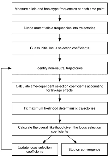
At the heart of our method is a maximum-likelihood calculation. Given a set of measurements from a system describing allele and two-locus haplotype frequencies at a range of different points in time (frequencies potentially being derived from individual sequences), we calculate the likelihood of these data given an arbitrary set of locus selection coefficients. This provides an objective function, which can be maximized to obtain the maximum-likelihood set of locus selection coefficients. Figure 1 provides an over-view of the different steps of the method, which we now describe in more detail.

Measuring allele and haplotype frequencies

Given our population, we consider changes in the popula-tion over time. At a given time t, we defineqa

iðtÞ to be the

frequency of the allelea2{0, 1} at locusiandqab

ij ðtÞto be

the frequency of the two-locus haplotypea,b2{0, 1} at loci i,j. We now suppose that the population is sampled at a set of time points tk for k ¼ 1, 2,. . ., with ngðtkÞ individuals

being sequenced at timetk.We writeq^aiðtkÞfor the sampled

frequency of the allelea 2{0, 1} at locus iat timetk,and

^ qab

ij ðtkÞas the sampled frequency of the two-locus haplotype

a,b2{0, 1} at locii,j, also at timetk.

Dividing mutant allele frequencies into trajectories

process, sample allele frequencies subsequent to the apparent fixation or death were examined.

Guessing initial locus selection coefficients

We use the notationfsi~gto describe the set of estimates of the locus selection coefficients {si}. Initial estimates for lo-cus selection coefficients were assigned from the uniform random distribution U(2s,s).

Identifying nonneutral trajectories

As we go on to describe, our method attempts to identify the strength of selection on an allele from observations of changes in the allele frequency, making the assumption that changes in allele frequency are driven primarily by selection. This assumption makes sense only if selective effects are indeed the main cause of allele frequency changes. We note that, at very small frequencies, changes in an allele fre-quency are dominated by genetic drift, with selection becoming the primary driver of evolution at a threshold frequency of 1/Ns(Rouzineet al.2001). To avoid assigning selection to primarily stochastic events, observed trajectories were divided into two sets according to their maximum ob-served frequency. Given an estimated locus selection coeffi -cient si~, trajectories at the locus i with a maximum allele frequency of less than a thresholdq_si¼minf1=Nsi~; 

1 10g, or

,1

10for~si#0, were modeled as evolving neutrally, the value

ofNhere being taken from the underlying population. Tra-jectories above this threshold were modeled as evolving nonneutrally, due to the effects of selection. While not elim-inating drift from the system, this removed from consider-ation a substantial number of trajectories for which selection was not the primary driver of allele frequency change.

Calculating time-dependent selection coefficients accounting for linkage effects

Due to effects such as hitchhiking and clonal interference, the selection acting on a mutant allele can change over time. We define the effective selection coefficient seiðtkÞ as the

selection acting on a mutant allele at locus i at time tk,

accounting for linkage to alleles at other loci under positive or negative selection. Assuming an additive model of selec-tion, the effect of linkage with other alleles can be written as a sum of pairwise interactions, such that

se

iðtkÞ ¼siþ X

j

sijðtkÞ; (1)

wheresij(tk) is the effect that alleles at locusjhave on the

selection acting on the mutant allele at iat timetk.

To demonstrate this, we first recall the standard result that, assuming deterministic dynamics, changes in the two-locus haplotype frequencies can be written in the form

_

qab_ab¼f_ijabqab_ij 2qab_ij 0

@ X

a9;b92f0;1g

f_ija9b9qa_ij9b9 1

A_; (2)

where a dot denotes a time derivative,fijab denotes thefi

t-ness of the respective two-locus haplotype, and the term in parentheses is the mean fitness. We now consider the de-velopment of the frequency of a mutant allele at locus i given a simultaneous polymorphism at locus j. At the locus i, the change in the mutant allele frequency can be expressed as

_

q1i ¼q_11ij þq_10ij : (3)

Combining this with the equation above, and using the assumption of additivefitness, we obtain

_

q1_i ¼siþsj

q11

ij þsiq10ij 2

q11 ij þq10ij

  · hsiþsj

q11_ij þsiq10_ij þsjq01_ij i

: (4)

Collecting terms insiandsjand rearranging gives

_ q1i ¼si

h

q11ij þq10ij 2

q11ij þq10ij 2i

þsj h

q00ij q11ij 2q10ij q01ij i

;

(5)

which with further rearrangement gives the form

_ q1i ¼

"

siþsj q11

ij q11

ij þq10ij

2 q

01 ij q01

ij þq00ij !#

q1i

12q1i

: (6)

Noting that, in a single-locus case, changes in the mutant allele frequency can be written as

_

q1i ¼siq1i

12q1i

; (7)

we obtain the result

sijðtkÞ ¼sj

q11 ij ðtkÞ q11

ij ðtkÞ þq10ij ðtkÞ

2 q

01 ij ðtkÞ q01

ij ðtkÞ þq00ij ðtkÞ !

: (8)

While only two interacting loci are considered here, Equation 8 is correct for multiple interacting loci (for derivation repeat the above calculations for q_1i ¼q_

111

ijk þq_

110

ijk þq_

101

ijk þq_

100

ijk ).

These equations are part of the standard population genetic toolkit and as shown above are straightforward to derive from Equation 2 (for a thorough treatment of multilocus systems including equations for the time evolution of the linkages, see Barton and Turelli 1991; Kirkpatrick et al.2002; Neher and Shraiman 2011).

For trajectories with maximal frequency less than the threshold frequency, the effective selection coefficients~e

iðtkÞ

was set to zero for each tk,while the effects of linkage

be-tween these and other trajectories were ignored; i.e.,

sijðtkÞ ¼0, where maxðq1jðtkÞÞ,1=Nsj. For all other

trajecto-ries, approximate time-dependent selection coefficientss~eiðtkÞ

were calculated from the estimated locus selection coeffi -cientsfsi~gand the sample haplotype frequencies^qab

ij ðtkÞ

us-ing Equations 1 and 8, to obtain a description of the selection acting on the mutant allele throughout the time for which it remained polymorphic.

Fitting maximum-likelihood deterministic trajectories

A deterministic curve, satisfying the approximate selection coefficientss~e

iðtkÞ, wasfitted to each trajectory. Under a

de-terministic scenario, if the locus i is the only polymorphic locus in the system, the evolution of q1

i has the analytical

solution

q1_iðtÞ ¼ q 1 ið0Þesit

12q1_ið0Þ þq1_ið0Þesit; (9)

whereq1

ið0Þis the frequency at timet¼0. Where more than

one locus in the system is polymorphic, changes in the haplotype frequencies and effective selection coefficients become interlinked, leading to complex evolutionary behav-ior; however, changes in the mutant allele frequency can be approximated using a discrete method. IfDtk¼tk+12tkis

small, such that the linkage between alleles does not change substantially within this time interval, we can write the dif-ference equation

q1_iðt_kþ1Þ ¼

q1 iðtkÞes

e

iðtkÞDtk

12q1

iðtkÞ þq1iðtkÞes e

iðtkÞDtk: (10)

This gives an approximation of the behavior of a mutant allele in a linked system under a deterministic scenario,

making the assumption of constant linkage between con-secutive sampling points.

Assuming the underlying frequencies q1

iðtÞ to evolve in

a deterministic manner according to selection, Equation 10 was applied to values of s~eiðtkÞ generated from the locus

selection coefficientsfsi~g. This gave, for each observed al-lele trajectory, a hypothetical mutant alal-lele trajectory f~q1iðtkÞg, approximating the evolution ofq1iðtÞ, in accordance

with the observed linkage between alleles, and obeying the calculated effective selection coefficients. Equation 10 defines a family of frequency curves, parameterized by q1

iðtkÞ for any one time point tk. For each trajectory, the

sampling time tc closest to equidistant between the start

and end points of the trajectory was found, and the fre-quency ~q1iðtcÞ was optimized to identify the deterministic

curve bestfitting the observed allele frequencies.

Curvefitting was carried out using a maximum-likelihood method, utilizing a binomial model. Given a large popula-tion in which the frequency of a mutant allele is q, the probability that a sample ofngsequences from the

popula-tion will have the mutant allele frequency^qis

P^q  q;ng

¼

ng ng^q

qng^qð12qÞngð12q^Þ: (11)

Considering a specific locus i at time tk, the likelihood of

a given underlying frequency q1

iðtkÞ given the observation

^ q1

iðtkÞcan be expressed as

Lq1_iðtkÞq^1iðtkÞ;ngðtkÞ

¼P^q1_iðtkÞq1iðtkÞ;ngðtkÞ

; (12)

while given multiple observed frequenciesf^q1

iðtkÞg, the log

likelihood of the underlying frequencies fq1

iðtkÞg can be

written as

logL q1iðtkÞ

¼X tk

logLðq1iðtkÞ^q1iðtkÞ;ngðtkÞÞ: (13)

For each trajectory, this equation was used to find the inferred frequenciesf~q1iðtkÞgbest approximating the

under-lying allele frequenciesfq1

iðtkÞg, whether the trajectory was

neutral or nonneutral. An illustration of the fitting process for a single polymorphism is shown in Figure 2.

Calculating the overall likelihood for the selection coefficients

Testing the performance of the method using model data

Having outlined the general principles of the method, we now describe its application to detect selection in a simulated population. A Wright–Fisher model was used to simulate a population offixed size, with loci divided into drivers, at which the mutant allele was under positive selection, and passengers, which evolved in a neutral fashion. Under a range of different model parameters, the ability of the

method to identify locus selection coefficients was tested. Details of the process are given below.

Simulating evolutionary histories:The underlying popula-tion was simulated using a Wright–Fisher model with afixed population size ofN¼104_{individuals. Each individual}

con-sisted of a sequence ofL¼50 binary loci,aij2{0, 1}, where

thefirst index denotes the individual (1#i #N) and the second denotes the locus (1#j#L). Loci themselves were divided into D driver loci, at which the mutant allele had some selection coefficients.0, andL2Dpassenger loci, at which the mutant allele had no selective advantage. An additivefitness landscape was assumed, such that thefitness Fiof an individual in the population was defined as the sum

of its allele fitnessesfa

j:

Fi¼X L

j¼1 faij

j : (14)

Within each generation, the alleles of any individual were subject to mutation from 0 to 1 or vice versa with fixed probability m defined by 2Nm ¼0.01. Subsequent genera-tions were sampled from the previous population using a multinomial sampling process, in which the probability pi of choosing an individual i for replication was

propor-tional to eFi_{. Simulations were carried out using a range of}

values of D2 f5; 10; 15; 20; 25; 50g and with 2Ns2 f10; 20; 50; 100g. In each case the evolution of the population was recorded over 4 million generations. For each combination of parameters {D, 2Ns}, five simu-lated population histories were generated.

In viral systems such as influenza, selective pressure on antigenic loci varies according to immune adaptation to the current strain. Here, a model of constant selective pressure on the driver loci was assumed, such that any new allele is always under selective advantage. As such, when a mutant allele at some locusfixed in the population, the frequency of the mutant was kept atfixation, removing the possibility of back mutations, for 3200 generations, the mutant frequency then being set to zero. The value of 3200 generations was picked arbitrarily, but allowed, with the exception of very long sample times,fixation events to be detected. Resetting fixed mutant allele frequencies in this manner caused difficulties in calling trajectories that would not be encoun-tered with biological sequence data; details of the solution applied in this instance are given inSupporting Information,

File S1.

Generating sample populations: A sample of constant size ng individuals was drawn from the population at regular

intervals of dtsgenerations, across a total ofTgenerations.

The occurrence and development of polymorphisms at each of the loci in the system were recorded, along with two-locus haplotype frequencies at each sample point.

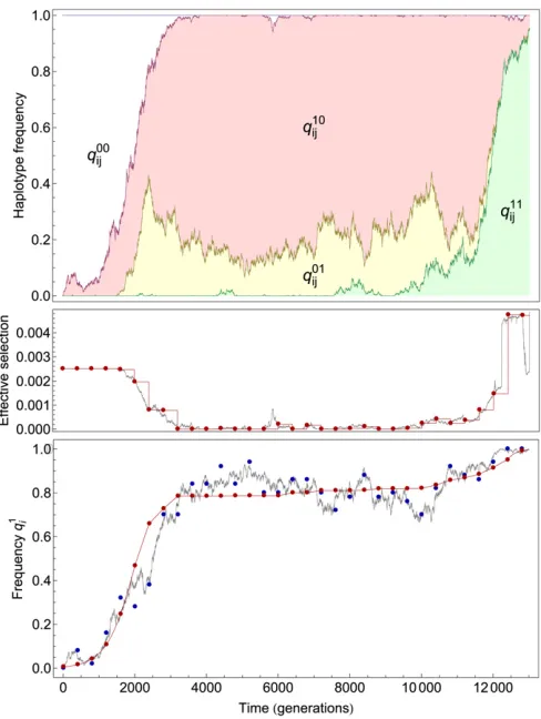
Figure 2 Illustration of the method of assigning a likelihood to a set of locus selection coefficients. Data are presented for a single trajectory in a model two-locus system. Top: Two-locus haplotype frequencies (colored lines) are sampled at each point in time. Middle: The sample two-locus haplotype frequencies, along with current estimates of the locus selection coefficients, are used to approximate the time-dependent effective selec-tion coefficientsse

iðtkÞfor the trajectory that has reachedfixation. Red

dots indicate the estimated selection coefficient, s~e

iðtkÞ, at each time

point, while the accompanying red line gives the approximate selection coefficient propagated over time (i.e., the selection is kept constant until the next sample). The real effective selection coefficient,se

iðtkÞ, measured

directly from the simulation, is represented by the gray line. Correct locus selection coefficients (si¼0.0025) have been used to calculate the

esti-mates shown. Bottom: Deterministic curves satisfying these selection coefficients arefitted to the observed allele frequencies using a maxi-mum-likelihood method. Observed allele frequencies ^q1

iðtkÞare shown

as blue dots. Estimated allele frequencies~q1_iðtÞare shown as red dots, with the accompanying red line describing the estimated propagation of the allele frequency. The true allele frequencyq1

iðtÞis shown as a gray

line. The log likelihood for the trajectory was obtained from thefit be-tween the~q1_iðtkÞand^q1iðtkÞvalues. Summing the log likelihoods over all

Fitting deterministic trajectories: To enable fitting be-tween the inferred and observed frequencies in the case of very short polymorphisms (the extreme case being a single observation), null “observations” of zero frequency were added to the start of each trajectory, with further observa-tions, representing fixation or death as appropriate, being added to the end of the trajectory. The number of observa-tions,no, added in each case was calculated as a function of

the difference between sample times across the trajectory, dts, and the mean time tofixation of a trajectory across the

simulation,tfix, each measured in generations

no¼max

tfix 10dts;   10

: (15)

Additional observations were added at intervals of dts. At

these additional sample times, for trajectories identified as being nonneutral, effective selection coefficients were set to the locus selection coefficient if the deterministic estimate for the wild-type frequency was in the interval½q_si; 12qsi

and to zero, representing neutral evolution, for allele fre-quencies outside of this interval. For trajectories not crossing the neutral threshold, effective selection coefficients were set uniformly to zero.

Simulated annealing:For each simulation, and each set of values {T,ng,dts},five separate annealing runs were carried

out, each beginning with a different set of estimates for the locus selection coefficientsfsi~g. At each step of the anneal-ing process, a trial change was made to a randomly chosen

~

siof magnitude chosen from a uniform random distribution. If the resulting change in log likelihood,D logL, was pos-itive, this change was accepted, while ifDlogLwas nega-tive the change was accepted with probabilityebDlogL_{for an}

annealing parameterb. In the case where a change in a locus selection coefficient led to a change in log likelihood of pre-cisely zero, the change was accepted if the new selection coefficient had a smaller magnitude than the previous selec-tion coefficient. This step implies the null hypothesis that each locus evolves under neutral selection; if no data were observed at a locus, it would be assigned close to zero se-lection. The annealing parameterbused in the evaluation of changes in likelihood was set to an initial value of 0.002, increasing by a factor of 1.005 each generation. In the event of 80 consecutive rejections of changes to fsi~gthe magni-tude of the random changes was decreased, the algorithm terminating after the third such set of rejections. In a sample set of calculations, across a variety of parameters, the mean standard deviation in a single optimized selection coefficient calculated across five annealing processes was 0.04, mea-sured in units of 2Ns.

Linked and unlinked analyses: Analyses of the simulated population data were carried out using two distinct meth-ods. In thefirst method, referred to from this point on as the

“linked method”, identification of selection coefficients was

carried out precisely as described in the methods above. In the second method, referred to as the “unlinked method”, selection coefficients were discerned without the inclusion of linkage, setting ~seiðtkÞ ¼si for all time points.

Compari-son of the results of the linked and unlinked methods gave an insight into the importance of linkage for correctly iden-tifying selection effects.

Analysis of results from model data

Having obtained predicted selection coefficients for each locus, two methods were applied to separate predicted driver loci from predicted passenger loci. In an initial measurement of the ability of the method to distinguish driver from passenger loci in a case where the number of driver loci is known to be equal to D, the loci with the D highest selection coefficients were identified as drivers, the remaining L2Dloci being identified as passengers. Using this approach, receiver operating characteristic (ROC) curves were plotted, comparing true and false positive iden-tifications of drivers across cases in which the model had between 5 and 25 driver loci for a default set of parameters ng¼100 and dts¼100, representing 1% sampling of the

population in 1% of generations, andT¼5·105_{, for each}

value ofs. A comparison was made between results of the linked and unlinked methods. Optimized selection coeffi -cients obtained for driver and passenger loci were exam-ined, examining the effect of linkage on estimates of each of these values.

In a more thorough assessment of the performance of the method, a clustering algorithm was used to separate drivers from passenger loci. Loci with large negative selection coefficients (less than minus the mean absolute value of f~sig) were automatically classified as passengers, while remaining loci were separated using a K-means clustering method, identifying initial cluster centers as the two loci with estimated selection coefficients closest to 2Ns and zero, respectively. The accuracy of identifying drivers and passenger loci was then calculated from the numbers of correctly and incorrectly classified loci,

Accuracy¼ d

þ_þpþ

dþþd2þpþþp2; (16)

whered+_{is the number of correctly identified driver loci,p}+

selection coefficients obtained using the linked and unlinked methods.

Results

Measuring selection in a linked system

In general, a goodfit was observed between the frequencies inferred with the linked method and the observed allele frequencies. This is a nontrivial result as the inference is based on a deterministic approximation (see Methods) of a complex stochastic system. It is precisely due to this ap-proximate description of the dynamics that the inference problem remains computationally tractable.

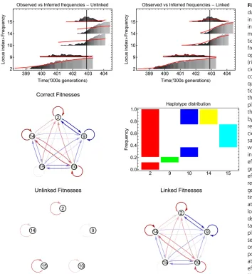
Figure 3 gives an illustration of the output generated by the inference at a single time point in a set of sample data. Comparison between the observed allele frequencies and those inferred shows errors where linkage between poly-morphisms was ignored, but a close fit where linkage was included. The inclusion of linkage in the inference accounts

for changes in the mutant allele’s effectivefitness caused by changes in the background population. The graph of correct fitness values and interlocus effects shows that linkage has a substantial effect on the locus selection coefficients and the resulting network of interactions is complex at the time point shown. While the mutant alleles at each of the 5 poly-morphic loci are all beneficial, the growth of the mutant at locus 9 is opposed by the influence of the beneficial alleles at loci 2, 10, 14, and 15, leaving it under strong negative se-lection. The mutant at locus 2, while opposed by the infl u-ence of the mutant allele at locus 9, is positively influenced by the mutant alleles at loci 10, 14, and 15, so retaining a strong positive selection.

The distribution of haplotypes gives some insight into thesefitness effects. While the beneficial allele at locus 9 is the only mutation in its haplotype, most other haplotypes contain two or more mutant alleles, and as such have higher fitnesses. Relative to the remainder of the population, the haplotype with the mutant at locus 9 is therefore under negative selection. By contrast, the haplotypes containing

Figure 3The linked method accurately repro-duces observed allele frequencies and underly-ing selection coefficients. Top: Observed and inferred allele frequencies for loci that are poly-morphic at the time point indicated by the ver-tical line of a simulated population. Allele frequencies inferred by the model (red lines), optimized using the unlinked (left) and linked (right) methods, are shown. Observed frequen-cies are plotted as gray columns, with lighter colors representing higher frequencies. Fre-quencies are stacked vertically, with the posi-tion on the vertical axis being calculated as the locus at which the polymorphism occurs, plus the frequency of the trajectory itself. Loci that are not polymorphic at the time indicated by the vertical line are not shown. Middle: Cor-rect values for time-dependent selection coeffi -cients and interlocus effects at the time of sampling (left). Nodes are labeled by locus, while directed edges between loci represent interlocus selection effects sij(t). Negative

effects, which decrease selection at the tar-geted locus, are colored blue, while positive effects, which increase selection, are colored red. In each case, darker colors represent stron-ger effects. Self-directed edges represent the time-dependent effective selectionse

iðtÞacting

the mutant at locus 2, which span the majority of the population, are on average positively selected for, resulting in positive selection on the mutant at locus 2.

Graphs illustrating effective selection evaluated from the inferred selection coefficients show the ability of the linked method to capture interference between mutations and more generally the importance of linkage in the evolution of the system. At the time point in question, the unlinked method infers loci 2, 14, and 15 to be under weak positive selection, while loci 9 and 10 are close to neutral. Under the linked method, however, the inferred pattern of selection and linkage between loci is close to being correct, with, for example, locus 9 under strong negative selection and locus 15 close to neutral.

We note here that the inferred selection coefficients represented in the graphs have been evaluated from the entire data set, rather than simply for this time window. Differences between the values obtained through the linked and unlinked methods therefore reflect, to some extent, the ability of these models to explain the whole of the data. Replicas of the three graphs, in which numerical values for the effective selection acting on each locus and the effects on the effective selection resulting from each pairwise interac-tion between loci are shown, are given inFigure S1.

Comparison of selection coefficients obtained with and without the incorporation of linkage

Examination of selection coefficients inferred with the linked method showed an improvement in two character-istics. First, driver loci inferred using the linked method had substantially more accurate (higher) selection coefficients than those obtained with the unlinked method. This is due to the former method accounting for clonal interference. Second, passenger loci at which a fixation occurred were inferred to have significantly lower selection coefficients under the linked method compared to the unlinked method. This result arises because the linked method can detect hitchhiking of neutral alleles with drivers.

Under the default parameters for the sampling process, 100 individuals were sampled from the population every 100 generations for a total of 5 · 105 _{generations. With}

these parameters, using the method of taking theDloci with the highest selection coefficients to identify drivers, the linked method showed a large improvement over the un-linked method in its ability to discern driver from passenger loci. Figure 4 shows ROC curves for the default model for various values ofs, the selection coefficient acting on driver loci in the population. Here, and throughout, this selection coefficient is expressed in terms of 2Ns, where N is the population size.

At each level of selection, the accuracy of the linked method was greater than that of the unlinked method. With 2Ns¼10, the calculated accuracies were 0.85 and 0.79 for the linked and unlinked methods, respectively, while with 2Ns¼50, the accuracies were 0.999 and 0.91. At the higher selection coefficients, the linked method separated driver and passenger loci almost perfectly.

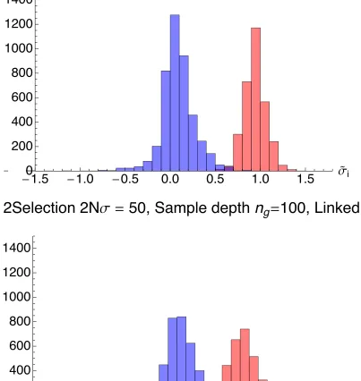
The histograms of selection coefficients identified with the linked and unlinked methods at 2Ns ¼50 showed a clear improvement by the former method in the assignment of selection coefficients to driver loci. Under the linked method, inferred selection coefficients of drivers and passengers were well separated into roughly Gaussian distributions, with clus-ters close to 0 and 1 (in units of 2Ns), with mean selection coefficients for driver and passenger loci of 0.94 and 0.08, respectively. Under the unlinked method, the distribution of the inferred driver loci selection coefficients had a substan-tially lower mean of 0.41 resulting from the failure to recog-nize clonal interference between drivers, while the mean of the passenger loci selection coefficients was 0.07.

Although no significant difference between methods was seen between mean selection coefficients for passenger loci, an improvement was seen under the linked method in the assignment of selection coefficients for passenger loci at which a fixation event took place, with substantially lower

Figure 4 Incorporation of linkage greatly improves dis-crimination between driver and passenger loci. Top: ROC curves for the default model system sampled over 5·105

mean selection coefficients being assigned.Figure S2shows mean optimized selection coefficients for this subset of loci.

Performance of the method across varying sampling parameters

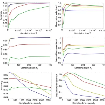
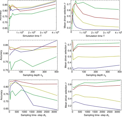
The performance of both methods was tested across a range of sampling parameters, the accuracy in identifying drivers and passengers being quantified using a clustering method, and selection coefficients being measured for driver loci. Results for the linked method are shown in Figure 5, with equivalent numbers for the unlinked method shown in

Figure S4. For each parameter set, five different sets of sample frequencies were generated from the evolutionary history of the population. These sets of frequencies were analyzed infive independent runs of the annealing process, so that each point in the figure represents a mean over at least 125 calculations (averaging also over at leastfive val-ues ofD). While statistical noise is still evident in the data, the overall trends are captured by the analysis.

The ability of the linked method to distinguish driver from passenger loci increased as the amount of sampling data increased, here quantified in terms of the number of generations sampled, T. Accuracies were higher at larger selection coefficients, due primarily to the increased differ-ence between driver and passenger loci, but also because of

the greater amount of information available for highly se-lected driver loci. At large selection coefficients, the proba-bility of a mutant allele escaping genetic drift is increased, leading to a larger number of observedfixation events. Fur-thermore, fixations occur more quickly, allowing for more fixations to occur in a given time. In the simulation run here, a mean of 2.71fixations per 105_{generations were observed}

in each driver locus for 2Ns= 100, but only 0.38fixations in the same time period for each driver locus for 2Ns= 10. For 2Ns= 100, an accuracy of.0.95 was observed after 75,000 generations. The same result was observed for 2Ns= 50 at 2 · 105 _{generations, while the accuracy for 2Ns = 20 is}

close to 0.95 after 1 million generations. As T increased, the accuracy of the method increased, representing better discrimination between drivers and passengers with more information available to the method. Perfect discrimination between driver and passenger loci was observed after 1 million generations for 2Ns= 100. Results obtained with the unlinked method were substantially worse, with an ac-curacy of ,0.85 for all selection coefficients tested after 2 million generations.

Variance in the accuracy of the linked method for varying values of the sample sizengshows roughly constant

perfor-mance for sample sizes .100, with a decrease in perfor-mance at smaller sample sizes. At the highest selection

Figure 5 Performance of the linked

method under varying data collection scenarios. Variation in the accuracy of the method in identifying driver and passenger loci (left column) and in the reproduction of selection coefficients (in units of 2Ns) for driver loci (right col-umn) is shown. Default parameters were a number of generations sampled ofT¼

5·105_{, a sampling depth ofn}

g¼100,

and a sampling frequency ofdts¼100

generations. Top: Variation in perfor-mance under different values of T, the number of generations sampled. Mid-dle: Variation in performance under dif-ferent values of ng, the number of

individuals sampled at each time point. Bottom: Variation in performance given different values ofdts, the time between

coefficients, good results are obtained at a sample size of 20, with accuracies of 0.97 achieved for 2Ns¼100 and 2Ns¼ 50; however, accuracy is rapidly lost below this point. Com-parison of locus selection coefficients obtained from simula-tions withng¼5,ng¼100, and 2Ns¼50 suggested poorer

accuracy at the lowest sampling level resulted from an in-crease in the variance of the inferred locus selection coeffi -cients. Details are shown inFigure S3.

The accuracy of the linked method showed dramatic changes with increased time between sampling points, dts.

At short sampling times, as already observed, high accura-cies can be achieved. However, asdtsincreases, a decline in

performance is seen, with an increased rate of decline at higher selection coefficients. At very long intervals between sample points, little information is collected about each tra-jectory, such that, in the extreme case,fixations are observed as changes in frequency from 0 to 1 at subsequent sample points. In such cases, measurements of linkage either cannot be made or become highly inaccurate when extrapolated over the time between sample points.

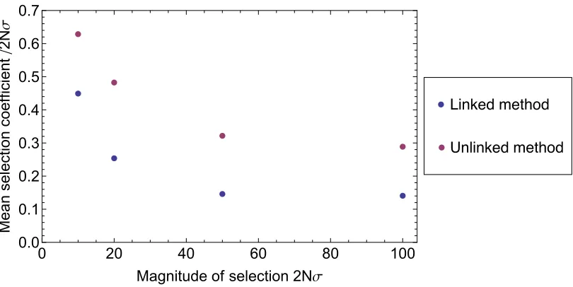
In systems for which every locus was a driver, improved selection coefficients were observed with the linked method compared to the unlinked method. Under the default sampling parameters, selection coefficients were mated using the unlinked method, with a larger underesti-mate at high selection coefficients. Mean inferred selection coefficients (in units of 2Ns) varied from 0.29 at 2Ns¼100 to 0.63 at 2Ns ¼ 10. Under the linked method, mean inferred selection coefficients for the all-driver case varied from 0.91 to 1.00, with no clear correlation between the inferred coefficient and the size ofs.

Interestingly, analysis of the selection coefficients ob-tained for driver loci reveals a systematic error in the coefficients obtained. AsTincreases, the mean selection co-efficient appears to tend to a limit that is less than one, with values closer to one obtained at lower selection coefficients. As dts increases, a dramatic fall in mean selection coeffi

-cients is seen, again with greater errors at higher selection coefficients. An explanation for this is discussed next.

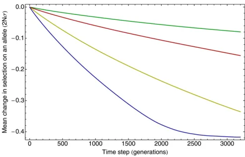
Interference reduces thefitness of mutations

Supposing the existence of a polymorphism at locus i, the function SiðtÞ was defined as the difference between the meanfitnesses of sequences in the population with and with-out the mutant allele at locusiat some timet. Furthermore, the change in the selective benefit of the mutant allele at i after some timet, resulting from changes in polymorphisms at other loci, is given bySiðtþtÞ2SiðtÞ. Figure 6 shows the mean of this statistic over all polymorphisms and all time steps t calculated directly from simulations with 20 driver loci and a varying driver selection coefficient. Averaged over all polymorphic observations, the real change in selection is negative, indicating that the selective advantage of a mutant allele generally decreases with time. Because of this, the as-sumption made in the method that the effective selection

coefficient will remain constant between sample points will, on a statistically consistent basis, produce an overestimate of the selective effects in the system. This overestimate, while initially small, increases as the interval between sample points increases both with the time interval t and with an increasing selection coefficient. When selection coefficients are optimized, therefore, the increased selection coefficient generated by the constantfitness assumption will be compen-sated for by reducing the inferred selection coefficient, the lower selection coefficient combining with the overestimate of selection over time to recreate the behavior of the system.

Discussion

We have given examples of the use of a method for quantifying selection in driver–passenger systems and dem-onstrated its potential to separate driver from passenger loci in a model system. By accounting for the background set of polymorphisms on which a trajectory develops, the linked method corrects for clonal interference, which can reduce apparent selection coefficients, and, through recognition of fixation events occurring through hitchhiking with driver alleles, assigns lower selection coefficients to passenger loci at which the mutant allele reachesfixation.

Unsurprisingly, the performance achieved in separating driver and passenger loci depended to a great extent on the magnitude of selection acting on the driver loci, a greater driver selection coefficient describing a greater inherent difference between the two classes of loci. Here, a driver selection coefficient of 2Ns $ 50 led to accuracies .95% under a range of conditions, while drivers at 2Ns= 20 were more difficult to distinguish.

Variation in the sampling parameters gave a range of results. Under variation in the length of the simulation, an

Figure 6 Interference decreases thefitness of a mutant allele over time. The mean change in the difference infitness between sequences, with the mutant or the wild-type allele at a given locus in the sequence, is measured as a function of time. Changes in the selection coefficient are measured in units of 2Ns. Data were calculated acrossfive simulations of length 2·106_{generations containing 20 driver and 30 passenger loci}

under varying selection coefficients and for selection coefficients 2Ns¼

increase in the available data consistently improved perfor-mance. With an underlying selection coefficient defined by 2Ns¼100, an accuracy of.0.95 in separating driver from passenger loci was achieved in a 50-locus model after 75,000 generations of sampling, captured by 750 sample points, each containing 100 individuals. Under variance in the depth of sampling, consistent accuracy was achieved down to locus sample sizes of 20, well within the reach of next-generation sequencing methods. Finally, where the time between consec-utive samples was varied, while good results were achieved at high sampling rates, increasing the sampling time was detri-mental to the accuracy achieved. At the higher selection coef-ficients,.95% accuracy was achieved up to a sample time of 400 generations, representing the collection of, on average, 10.7 and 6.2 samples within the mean time for a fixation event at 2Ns¼50 and 2Ns¼100, respectively.

Reproducing precise values of selection coefficients proved a challenge, with the assumption of constant selection between sampling points leading to a systematic underesti-mate in the coefficients assigned to driver loci. Due to the computational and theoretical difficulties inherent in mod-eling stochastic evolution of multiple linked loci over a number of generations, some form of approximation to model the selection acting on trajectories between sampled time points is necessary [evaluation of selection using a trajectory including stochastic effects has been carried out in a single-locus case (Bollbacket al.2008)]. We leave the task of improving on the constant selection between the sample points approximation to future work.

Considering the application of the method to specific examples of experimental data, we note that care must be taken in the interpretation of the parameters discussed above and their effect on the accuracy potentially achievable. For the number of generations sampled, while the amount of information available increases linearly with time, the rate of this increase is a function of the inherent properties of the system. Under a higher mutation rate, more events would be observed per generation, such that more information would be available in a set number of generations. Whereas if the selection coefficient was increased, more mutations in driver loci would escape being removed at low frequencies by genetic drift, such that more fixation events would be seen. Here, where division of the entire set of loci into driver and passenger sets was the goal, a large amount of data were required, with the observation of at least one significant event in a driver locus being necessary for its identification as a driver. Accounting for driver loci in which nofixation was observed improved results at low values of T (data not shown). Depending on what is desired to be learned from a system, and depending on the underlying dynamics of the system in question, the numerical values for parameters re-quired for a given accuracy may vary substantially.

For the purposes of method development we have here considered a simplified model of a viral genome under constant selective pressure at each locus. However, given the

caveats mentioned above, we suggest that the approach we present, with suitable modification, has the potential to be applied to a wide range of biological systems. While, as mentioned above, the use of genetic markers can be used to identify the fitness of subsets of a population (Lang et al. 2011), where a greater amount of sequence information is available, the effect of the genetic background on the de-velopment of individual alleles can be quantified. Even in systems for which a small number of mutations are ob-served, the core component of the method, offitting trajec-tories that obey an effectively time-dependent model of selection to observed allele frequencies, can be applied.

While many simplifications were made in the application of the inference method presented here, the method has potential to be extended in several directions. Considering biological data, with allowance for synonymous and non-synonymous mutations, the binary locus model used here could be extended. Replacement of the constant sampling time intervals and sampling depths with variable measures is easily implementable within the current framework.

More complex evolutionary scenarios could also be mod-eled. For example, while recombination decreases linkage between alleles, disrupting the driver–passenger paradigm considered here, it would not necessarily prevent application of the method. If the rate of recombination were low relative to the rate of sampling, estimates of linkage captured by haplotype sampling would still be accurate enough to provide a meaningful picture of linkage between polymorphisms until the next sample was taken, thereby allowing for improved discernment of selection in the system.

Acknowledgments

We thank Stephan Schiffels for advice regarding the implementation of the Wright–Fisher model and partici-pants of the Kavli Institute of Theoretical Physics (KITP) program on Microbial and Viral Evolution for discussions. We acknowledge the Wellcome Trust for support under grant 091747. This research was also supported in part by the National Science Foundation under grant NSF PHY05-51164 during a visit at the KITP (Santa Barbara, CA).

Literature Cited

Barrick, J. E., D. S. Yu, S. H. Yoon, H. Jeong, T. K. Oh et al., 2009 Genome evolution and adaptation in a long-term exper-iment with Escherichia coli. Nature 461(7268): 1243–1247. Barrick, J. E., M. R. Kauth, C. C. Strelioff, and R. E. Lenski,

2010 Escherichia coli rpoB mutants have increased evolvabil-ity in proportion to theirfitness defects. Mol. Biol. Evol. 27(6): 1338_–1347.

Barton, N. H., 1995 Linkage and the limits to natural selection. Genetics 140(2): 821–841.

Barton, N. H., and M. Turelli, 1991 Natural and sexual selection on many loci. Genetics 127(1): 229–255.

Betancourt, A. J., 2009 Genomewide patterns of substitution in adaptively evolving populations of the RNA bacteriophage MS2. Genetics 181(4): 1535–1544.

Bollback, J. P., and J. P. Huelsenbeck, 2007 Clonal interference is alleviated by high mutation rates in large populations. Mol. Biol. Evol. 24(6): 1397–1406.

Bollback, J. P., T. L. York, and R. Nielsen, 2008 Estimation of 2Nes from temporal allele frequency data. Genetics 179: 497–502. Chare, E. R., 2003 Phylogenetic analysis reveals a low rate of

homologous recombination in negative-sense RNA viruses. J. Gen. Virol. 84(10): 2691–2703.

Cof_fin, J. M., 1995 HIV population dynamics in vivo: implications for genetic variation, pathogenesis, and therapy. Science 267 (5167): 483–489.

de Visser, J. A. M., C. W. Zeyl, P. J. Gerrish, J. L. Blanchard, and R. E. Lenski, 1999 Diminishing returns from mutation supply rate in asexual populations. Science 283(5400): 404–406.

Desai, M. M., and D. S. Fisher, 2007 Bene_ficial mutation selection balance and the effect of linkage on positive selection. Genetics 176(3): 1759_–1798.

Fisher, R. A., 1930 The Genetical Theory of Natural Selection. Clar-endon Press, Oxford.

Gerrish, P. J., and R. E. Lenski, 1998 The fate of competing ben-e_ficial mutations in an asexual population. Genetica 102_–103 (1–6): 127–144.

Gillepie, J. H., 2001 Is the population size of a species relevant to its evolution? Evolution 55(11): 2161_–2169.

Grenfell, B. T., O. G. Pybus, J. R. Gog, J. L. N. Wood, J. M. Daly

et al., 2004 Unifying the epidemiological and evolutionary dy-namics of pathogens. Science 303(5626): 327_–332.

Hegreness, M., N. Shoresh, D. Hartl, and R. Kishony, 2006 An equivalence principle for the incorporation of favorable muta-tions in asexual populamuta-tions. Science 311(5767): 1615–1617. Holland, J., K. Spindler, F. Horodyski, E. Grabau, S. Nicholet al.,

1982 Rapid evolution of RNA genomes. Science 215(4540): 1577–1585.

Kao, K. C., and G. Sherlock, 2008 Molecular characterization of clonal interference during adaptive evolution in asexual popu-lations of Saccharomyces cerevisiae. Nat. Genet. 40(12): 1499– 1504.

Kirkpatrick, M., T. Johnson, and N. Barton, 2002 General models of multilocus evolution. Genetics 161: 1727–1750.

Lang, G. I., D. Botstein, and M. M. Desai, 2011 Genetic variation and the fate of bene_ficial mutations in asexual populations. Ge-netics 188: 647–661.

Muller, H. J., 1932 Some genetic aspects of sex. Am. Nat. 66 (703): 118–138.

Mustonen, V., and M. Lässig, 2009 From fitness landscapes to seascapes: non-equilibrium dynamics of selection and adapta-tion. Trends Genet. 25(3): 111_–119.

Neher, R. A., and B. I. Shraiman, 2011 Statistical genetics and evolution of quantitative traits. Rev. Mod. Phys. (in press). Park, A., J. Daly, N. Lewis, D. Smith, J. Wood et al.,

2009 Quantifying the impact of immune escape on transmis-sion dynamics of influenza. Science 326(5953): 726–728. Park, S.-C., D. Simon, and J. Krug, 2010 The speed of evolution in

large asexual populations. J. Stat. Phys. 138(1_–3): 381_–410. Perfeito, L., L. Fernandes, C. Mota, and I. Gordo, 2007 Adaptive

mutations in bacteria: high rate and small effects. Science 317 (5839): 813–815.

Rouzine, I., A. Rodrigo, and J. Coffin, 2001 Transition between stochastic evolution and deterministic evolution in the presence of selection: general theory and application to virology. Micro-biol. Mol. Biol. Rev. 65(1): 151–185.

Rouzine, I. M., J. Wakeley, and J. M. Coffin, 2003 The solitary wave of asexual evolution. Proc. Natl. Acad. Sci. USA 100(2): 587–592. Smith, D. J., A. S. Lapedes, J. C. de Jong, T. M. Bestebroer, G. F. Rimmelzwaanet al., 2004 Mapping the antigenic and genetic evolution of in_fluenza virus. Science 305(5682): 371_–376. Smith, J., and J. Haigh, 1974 The hitch-hiking effect of a

favour-able gene. Genet. Res. 23(01): 23–35.

Sniegowski, P. D., and P. J. Gerrish, 2010 Beneficial mutations and the dynamics of adaptation in asexual populations. Philos. Trans. R. Soc. B Biol. Sci. 365(1544): 1255–1263.

Stephan, W., and C. H. Langley, 1989 Molecular genetic variation in the centromeric region of the X chromosome in three Dro-sophila ananassae populations. I. Contrasts between the vermil-ion and forked loci. Genetics 121: 89–99.

Stratton, M., P. Campbell, and P. Futreal, 2009 The cancer ge-nome. Nature 458(7329): 719_–724.

Weinreich, D. M., R. A. Watson, and L. Chao, 2005 Perspective: sign epistasis and genetic constraint on evolutionary trajecto-ries. Evolution 59(6): 1165–1174.

Wilke, C. O., 2004 The speed of adaptation in large asexual pop-ulations. Genetics 167: 2045–2053.

GENETICS

Supporting Information

http://www.genetics.org/content/suppl/2011/09/07/genetics.111.133975.DC1

Distinguishing Driver and Passenger Mutations in

an Evolutionary History Categorized by Interference

Christopher J. R. Illingworth and Ville Mustonen

Distinguishing driver and passenger mutations in an

evolutionary history categorized by interference

Christopher J. R. Illingworth

1

_{and Ville Mustonen}

1,∗

_,

1 Wellcome Trust Sanger Institute, Hinxton, Cambridge, UK

∗

E-mail: Corresponding [email protected]

SUPPORTING TEXT

Calling trajectories

The resetting of fixed mutant alleles led to di

ffi

culties in calling

trajectories which would not be encountered with biological sequence data, particularly in

identifying the end of a trajectory. While, in the identification of the initial point of a

trajectory, ignoring sampling e

ff

ects makes for a pragmatic solution, the time of fixation or

death of a polymorphism is more di

ffi

cult to pinpoint. Indeed, errors at this point can lead

to the spurious identification of new trajectories, leading to obvious problems in the later

analysis. Here, a cuto

ff

number of observations,

c

, was defined as

c

=

max

{

300

/

n

g

,

8

}

(1)

In the case of an apparent death of a polymorphism at some locus

i

, indicated by a zero

sample frequency, the frequencies

q

ˆ

1

i

(

t

k

)

at the subsequent

c

−

1

samples were examined. If

a non-zero sample frequency was observed in any of these samples, it was assumed that the

apparent death was an artefact of limited sampling, and the polymorphism was assumed to

be in existence across the intervening time-points. If no non-zero sample frequencies were

observed, the apparent observation of the death of the wild-type allele was assumed to reflect

a death in the underlying population. The value of 300 used in the definition of

c

here reflects

the number of observations required to be 95% certain that a polymorphism does not exist

at a frequency greater than 1% in the underlying population. In the case of an apparent

fix-ation in the populfix-ation, marked by a sample frequency value of 1, a slightly di

ff

erent process

was required, due to the delayed return in the simulation of fixed mutant alleles to the wild

type. Subsequent to an apparent fixation, the allele frequencies at the locus were observed

1

File
S1


Supporting
Information


C.
J.
R.
Illingworth
and
V.
Mustonen
 3
SI




as above. If a polymorphic frequency between 0 and 0.5 was observed at that locus, it was

assumed that the fixed mutant allele had been returned to the wild-type, and a fixation was

recorded at the first time of apparent fixation in the locus. If a polymorphic frequency greater

than 0.5 was observed at the locus, it was assumed that the initial observation of fixation

arose through limited sampling, no fixation having occurred in the intervening time. We note

that, at large values of

dt

s

, this method is not error-free in the histories of polymorphisms

called at di

ff

erent loci, leading to a potential worsening of the results reported in the main

text for long sampling times. However, when the method is extended to a biological

sys-tem, with binary alleles replaced by codons, the mutation of a fixed allele back to wild-type

would become easily distinguishable from a mutation to a new, third allele at the same locus.

SUPPORTING FIGURES

[Figure 1 about here.]

[Figure 2 about here.]

[Figure 3 about here.]

[Figure 4 about here.]

!57

!50

!8

!7

!6

!50 57

8 7

6

!23 23

48

!33 39

!21 21

!32

!3

!25

!14 14

30

!20

64 ₉

2

10 15

14

True Fitnesses

20

4

8 26

11

2

9

10 15

14

Unlinked Fitnesses

!49

!39

!6

!6

!5

!42 49

6 6

5

!18 18

39

!27 32

!17 17

!26

!2

!20

!11 11

24

!16

51 ₉

2

10 15

14

Linked Fitnesses
















































































































Figure
S1



Selection
and
inter‐locus
effects
in
a
model
system.
Details
of
selection
coefficients
in
the
system
represented
in
 Figure
2
of
the
main
text.
Red
edges
indicate
positive
selection
and
inter‐locus
effects,
while
blue
edges
indicate
negative
 selection
and
inter‐locus
effects.
The
data
represented
is
identical
to
that
in
the
graphs
of
Figure
2,
albeit
with
numerical
values
 included.
A
close
fit
between
the
true
selection
and
the
inferred
selection
using
linked
method
can
be
observed.

















0

20

40

60

80

100

0.0

0.1

0.2

0.3

0.4

0.5

0.6

0.7

Magnitude of selection 2N

Σ

Mean

se

le

cti

on

co

effi

ci

en

t

!

2N

Σ

Unlinked method

Linked method


























































Figure
S2


The
linked
method
more
accurately
measures
selection
in
passenger
loci
observed
to
undergo
fixation.
Mean
inferred
 selection
coefficients,
in
units
of
2Nσ,
assigned
to
loci
from
simulations
with
T
=
500,
ng
=
100,
and
dts
=
100,
for
various
values
of
 the
underlying
selection
coefficient
σ,
calculated
from
the
models
excluding
linkage
(purple),
and
including
linkage
(blue).
The
 correct
value
in
each
case
is
zero.
More
than
800
inferred
selection
coefficients
are
represented
by
each
data
point.
A
similar
 relationship
between
selection
coefficients
is
observed
for
different
values
of
the
parameters
T,
ng,
and
dts.





!

0

1.5

!

1.0

!

0.5

0.0

0.5

1.0

1.5

Σ#

i

200

400

600

800

1000

1200

1400

Selection 2N

Σ $

50, Sample depth

n

g

$

100, Linked

!

0

1.5

!

1.0

!

0.5

0.0

0.5

1.0

1.5

Σ#

i

200

400

600

800

1000

1200

1400

2Selection 2N

Σ $

50, Sample depth

n

g

$

100, Linked

























































































































Figure
S3






Selection
coefficients
inferred
from
lower
sampling
levels
had
a
greater
variance.
Inferred
selection
coefficients,
in
 units
of
2Nσ,
for
driver
(red),
and
passenger
(blue)
selection
coefficients
for
T
=
500,
dts
=
100,
and
ng
equal
to
100
and
5
 respectively.
The
greater
variance
at
lower
sampling
is
evident.
Outlier
passenger
coefficients
falling
lower
than
the
range
shown
 are
excluded
‐
these
comprise
3.5%
of
coefficients
at
ng
5
and
0.3
%
of
passenger
coefficients
at
ng
=
100.


0 _1!106 _2!106 _3!106 _4!106

0.65 0.70 0.75 0.80 0.85

Simulation time T

Accu

ra

cy

0 _1!106 _2!106 _3!106 _4!106

0.3 0.4 0.5 0.6 0.7

Simulation time T

Mean

d

ri

ve

r

se

le

cti

o

n

Σ#

0 100 200 300 400

0.70 0.75 0.80 0.85

Sampling depth ng

Accu

ra

cy

0 100 200 300 400

0.3 0.4 0.5 0.6 0.7

Sampling depth ng

Mean

d

ri

ve

r

se

le

cti

o

n

Σ#

0 500 1000 1500 2000 2500 3000 0.65

0.70 0.75 0.80

Sampling time$step dts

Accu

ra

cy

0 500 1000 1500 2000 2500 3000 0.2

0.4 0.6 0.8

Sampling time$step dts

Mean

d

ri

ve

r

se

le

cti

o

n

Σ#







































































































Figure
S4


Performance
of
the
unlinked
method
under
varying
data
collection
scenarios.
Variation
in
the
accuracy
of
the
method
 in
identifying
driver
and
passenger
loci
(left
column)
and
in
the
reproduction
of
selection
coefficients,
in
units
of
2Nσ,
for
driver
 loci
(right
column).
Default
parameters
were
T
=
5
×
105
,
ng
=
100,
and
dts
=
100.
Top:
Variation
in
performance
under
different
 values
of
T
,
the
number
of
generations
sampled.
Middle:
Variation
in
performance
under
different
values
of
ng,
the
number
of
 individuals
sampled
at
each
time
point.
Bottom:
Variation
in
performance
given
different
values
of
dts,
the
time
between
sample
 points.
Data
is
plotted
for
values
of
2Nσ
equal
to
100
(blue),
50
(red),
20
(yellow)
and
10
(green).
Accuracy
values
are
averaged
 over
simulations
with
5,
10,
15,
20,
and
25
drivers,
while
mean
sigma
values
are
averaged
over
simulations
with
5,
10,
15,
20,
25,
 and
50
drivers.