Hardware Implementation of a Low Power Speech Recognition System

(1)

ABSTRACT

PAZHAYAVEETIL, ULLAS CHANDRASEKHAR. Hardware Implementation of a Low Power Speech Recognition System. (Under the direction of Dr. Paul Franzon.)

Speech is envisioned as becoming an important mode of communication and interaction

with computing devices and systems in the future. The potential for speech recognition

applications both in our living environment as well as our workplace is well understood,

and is driving the shift from current command and control applications to full fledged

speech recognition systems. While these systems would be especially useful in future

mobile embedded domains, the real-time performance requirements of such systems

cannot be met by current embedded processors. Even modern high performance

microprocessors are barely able to keep up with the real time requirements of

sophisticated speech recognition applications often straining the resources of the host

processor while incurring a power consumption that is prohibitive in the embedded space.

Custom ASIC solutions in the past have focused on faster clock rates and logic speeds,

and have largely ignored the power reduction aspect of the problem. In this dissertation,

we approach the speech recognition problem by a) designing a custom ASIC that is

flexible enough to adapt to evolutionary improvements in the design and take advantage

of these improvements at the algorithmic level to achieve low power operation, and b)

restructuring the memory and adapting a lexical style dictionary along with an innovative

(2)

Our Gaussian Estimator achieves real-time performance while reducing power

consumption by 2 orders of magnitude over a software implementation running on a

Pentium 4 processor, and by 43% over the best previous comparable ASIC design. Our

design also achieves 3 orders of magnitude improvement in energy consumption over the

Pentium 4 and 35% improvement in energy consumption over the previous ASIC design.

Similarly our Viterbi Decode unit performs real-time speech recognition while

achieving an improvement of 3 orders of magnitude over the Pentium 4 and 1 order of

magnitude improvement over the previous design – the perception processor – in both

power and energy savings.

Our final design achieves real-time recognition over a vocabulary that is 6-12

(3)

HARDWARE IMPLEMENTATION OF A LOW POWER SPEECH RECOGNITION SYSTEM

by

ULLAS CHANDRASEKHAR PAZHAYAVEETIL

A dissertation submitted to the Graduate Faculty of North Carolina State University

in partial fulfillment of the requirements for the Degree of

Doctor of Philosophy

ELECTRICAL ENGINEERING

Raleigh, North Carolina

2007

APPROVED BY:

_________________________ _________________________

Dr. Suleyman Sair Dr. Min Kang

__________________________ _________________________

Dr. Paul Franzon Dr. W. Rhett Davis

(4)

DEDICATION

Two very special people have been responsible for helping me complete this work, and

their contribution began far before I even joined this project. They are the two greatest

people I know and whom I have the privilege of proudly calling my parents – Mr.

Chandra Sekhar and Mrs. Rajalakshmi Chandra Sekhar. This dissertation is a testament to

their foresight, love, support and their willingness to sacrifice so that I never had to. None

(5)

BIOGRAPHY

Ullas Chandra Sekhar received his Bachelor of Technology in Electrical Engineering

from the Indian Institute of Technology, Madras in 2001. He was also awarded the Dr.

Ing Dieter Kind Prize for the best B.Tech project in Electrical Engineering for 2001. He

received his Master of Science in Electrical Engineering in 2003 from the University of

Texas at Arlington. During his MS program, he worked as a research assistant at the

Automation and Robotics Research Institute. He joined North Carolina State University

in 2003, where he worked both as a research assistant and a teaching assistant while

working towards his Ph.D. His research interests are primarily hardware and ASIC

(6)

ACKNOWLEDGEMENTS

I would like to thank my advisor, Dr. Paul Franzon, for his patient mentoring and

guidance through out this research. He managed to maintain the perfect balance between

giving me a free hand in exploring research ideas, and steering me towards focusing on

the core goals of the project. His confidence in this fledgling project during rough patches

and roadblocks, and his support both in matters relating to this research as well as outside

of it, have been two of the greatest assets to this research dissertation. I would also like to

thank the rest of my committee – Dr. Rhett Davis, Dr. Suleyman Sair, and Dr. Min Kang

– for their generous advice and help, especially in finding solutions to practical issues

that came up during the course of this research. Their open-door policy has been

extremely reassuring. I would like to thank my friends for providing a balance to my

lifestyle, which would otherwise have been ‘a graduate student’s life’. Last, but certainly

not the least, I would like to thank my family – my father Mr. Chandra Sekhar and my

mother Mrs. Rajalakshmi Chandra Sekhar, for their love, support and sacrifice, my

brother Unmesh who could not have cared less about the details of what I did, but

listened to me nevertheless just because it was important to me, and finally my fiancé

Gayathri for getting me through this last year, and lifting my spirits when things looked

(7)

LIST OF TABLES

Page

Table 5.1 - SRAM and DRAM specifications ………. 45

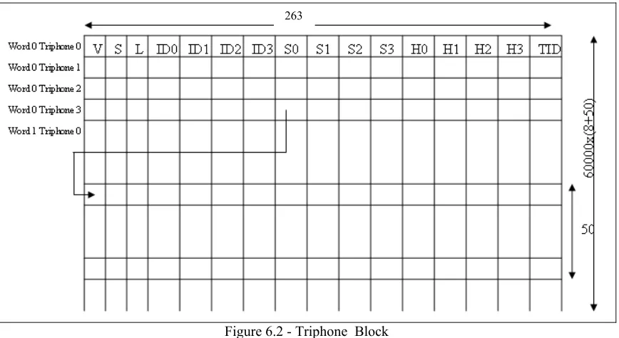
Table 6.1 - Contents of Triphone_Block ………. 60

Table 6.2 - Viterbi Decoder Memory Element Sizes ………... 71

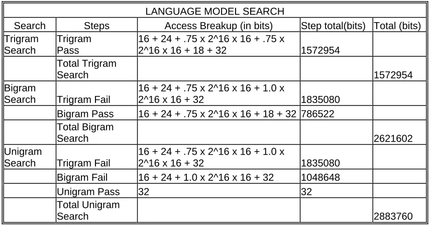
Table 6.3 - Language Model Search Access Breakup ………. 76

Table 6.4 - Triphone_block row bits (old and new) ……….... 81

Table 6.5 - Signals in the Viterbi Update Unit –1 ………. 106

Table 6.6 - Signals in the Initiator ………. 109

Table 6.7 - Signals in the MEM_Allocator ……….... 113

Table 6.8 - Signals in the Viterbi Update Unit –2 ………. 114

Table 7.1 - Memory Requirement Breakup comparison ………... 126

Table 7.2 - Memory access breakup for single frame ……… 128

(11)

LIST OF FIGURES

Page

Figure 1.1 - Performance of SPHINX 3 on Intel Pentium 3

and later processors (900MHz to 3GHz) ……… 3

Figure 1.2 - Performance and power considerations for speech recognition on modern architectures ……….. 4

Figure 2.1 - Schematics of an LVR (Large Vocabulary Recognition) system ……….. 9

Figure 2.2 - Hidden Markov Model ………. 10

Figure 2.3 - Block diagram of node representing state j ……….. 12

Figure 2.4 - Decoder structure showing forward computation and backtracking ….... 13

Figure 2.5 - HMM for word ‘HI’ ………. 17

Figure 2.6 - State-tying ……… 17

Figure 2.7 - Use of Language model …….………. 21

Figure 4.1 - System Overview ………. 36

Figure 4.2 - System Implementation Overview ………... 38

Figure 4.3 - Front-End ………. 39

Figure 5.1 - Baseline Gaussian Estimator ……….... 44

Figure 5.2 - Reduced Calculation Gaussian Estimator ……….... 46

Figure 5.3 - Gaussian Estimator Interfacing ……… 51

Figure 5.4 - Gaussian Estimator ……….. 53

Figure 6.1 - Flat vs. Lexical Dictionary .……….. 57

(12)

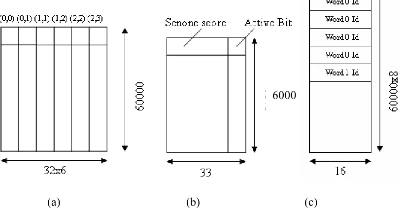
Figure 6.3 - (a) Transition_Block (b) Senone_Score (c) Word_Lookup …………... 62

Figure 6.4 - (a) Identified_Words (b) Last_Phone_Score ………. 63

Figure 6.5 - Update Unit ……….. 65

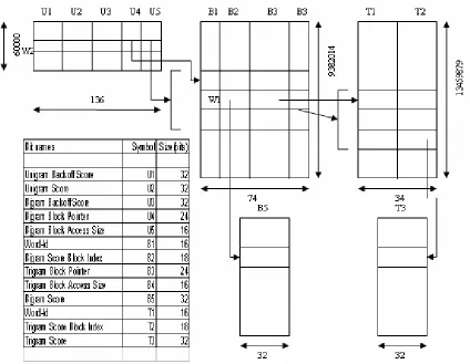
Figure 6.6 - Language Model Memory Blocks ……….... 69

Figure 6.7 - Memory access per frame ……….... 77

Figure 6.8 - Triphone_block row (old and new) ……….. 81

Figure 6.9 - Within-word transition example ……….. 82

Figure 6.10 - (a) temp_list (b) Identified_words ……….. 85

Figure 6.11 - Final 50 initialization ………. 87

Figure 6.12 - Viterbi Decoder and its interfacing ……… 92

Figure 6.13 - Phase 1 ……… 94

Figure 6.14 - Checking the Availability List and allocating space in Triphone_Block_Type_B ………. 96

Figure 6.15 - Phase 2 ……… 98

Figure 6.16 - Phase 3 ………... 99

Figure 6.17 - Phase 4 ……….. 100

Figure 6.18 - Senone Score Updating ……… 102

Figure 6.19 - DRAM Interfacing ………... 103

Figure 6.20 - The Viterbi Update Unit –1 ……….. 106

Figure 6.21 - Final 50 Initiator Unit – Initiator ……….. 109

Figure 6.22 - Initializing and updating Triphone_Block_Type_B ………. 111

Figure 6.23 - Final 50 Initiator Unit – MEM_Allocator ……… 112

(13)

Figure 6.26 - Language Model Unit ……….. 117

Figure 7.1 - GE Real Time Performance (speed) ……….. 122

Figure 7.2 - GE Power Consumption ………. 123

Figure 7.3 - Power Consumption across systems – Benchmark 1 ………. 124

Figure 7.4 - Process Normalized Energy Consumption across systems – Benchmark 1 ……… 124

Figure 7.5 - Final Implementation Memory Breakup ……… 126

Figure 7.6 - Initial Implementation Memory Breakup ………... 127

Figure 7.7 - Power Consumption across systems – Benchmark 2 ………. 130

(14)

CHAPTER 1 Introduction

Speech recognition has been an area of active research for more than 40 years [1],

maturing from an area of pure academic research to one with growing use in the

marketplace. Opportunities for application of speech recognition are immense and

diverse. The trend of a constantly increasing number of computing devices, both in our

living environment, as well as our workplace, calls for a better way of interacting with

them. Speech is already an established mode of communication in many mobile

embedded environments, and the value of speech recognition applications in such

environments is immeasurable. When compared to other forms of communication, speech

has some attractive advantages. A person can speak about 3-4 times faster than they can

type, allowing for greater communication efficiency. It is ideal for multi-modal tasks

since the hands and eyes are free to do other tasks. Speech accessories are cheap, easily

available and small, creating mobile capacity. Thus this hands-free, user friendly nature

of speech coupled with improvements in processor speeds and trends of ubiquitous

computing, promise to make speech a primary human/machine interface in the near

(15)

1.1 The Problem

A variety of software packages for speech recognition are available in the mass market

today, such as Dragon Systems' Dragon Naturally Speaking, IBM's ViaVoice, Lernout &

Hauspie's Voice Xpress, and Philips FreeSpeech98[2]. Vocabularies in commercial

systems today range from 20,000 to 150,000 words. Recognition accuracies have been

steadily improving as well, though current systems are still not sufficiently accurate to

easily take dictation without straining the resources of the microprocessor. The CMU

‘Speech in Silicon’[3] is another project that is working at developing a hardware

solution to speech recognition.

A successful design of a speech recognition system involves achieving accuracy

levels of >95% while being fast enough to be able to process speech in real time. The

system should be able to achieve speaker-independent speech recognition for multiple

languages. (i.e. the system must be deployed with base training (speaker independent

models) with update and training facilities). The system should be flexible enough to

handle different dialects and speech model parameters with minimal effort to change

dialects, ideally requiring only a download of a new model. Power savings have also

come to be of significant importance during the designing of such systems due to their

application in the embedded domain.

Even modern high performance microprocessors are barely able to keep up with

the real time requirements of sophisticated speech recognition applications. The run times

[4] for a 29.3 sec segment of speech over the SPHINX III speech recognition system is

shown in Figure 1.1. The theoretical run times are based on ideal scaling of performance

(16)

does not scale ideally. In theory a 2.4 GHz processor should achieve real time

performance. In practice a processor frequency of approximately 2.9 GHz is required to

satisfy real time requirements.

Figure 1.1 - Performance of SPHINX 3 on Intel Pentium 3 and later processors (900MHz to 3GHz)

This performance gap suggests that when moving to more complex future speech

recognition workloads higher frequencies alone are not the solution, fundamental

architectural improvements are called for. The speech recognition system also severely

limits the processor’s availability for other task. The results clearly show that speech

applications stress the performance limits of high-end processors.

By their very nature, applications such as speech are likely to be most useful in

mobile embedded systems. A fundamental problem that plagues these applications is that

they require significantly more performance than current embedded processors can

(17)

featured speech recognizer. The energy consumption that accompanies the required

performance level is often orders of magnitude beyond typical embedded power budgets.

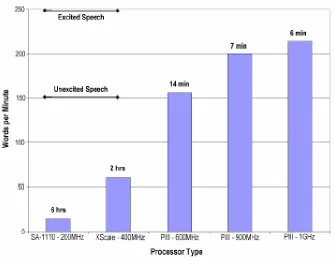
Figure 1.2 provides a rough estimate of the speech recognition rate achievable on various

modern computing systems [5]. Annotated above each bar is the time each processor

class would operate on a single “AA” rechargeable battery (1600 mA·Hr). It is clear that,

while high-end systems are within the performance range necessary for real-time speech

recognition, they far exceed the power budget of portable devices.

Figure 1.2 - Performance and power considerations for speech recognition on modern architectures

Another problem that these systems face especially in the mobile domain is that

with new and emerging techniques in speech recognition, it is more attractive to find a

solution that can readily adapt to most if not all of the developments and techniques.

Often many of these new techniques prove to be useful in more than one domain. As an

(18)

reduce both processing and power consumption as well as required memory bandwidth. It

is prudent to look into finding a way to incorporate these into our own system.

1.2 The Solution

The problem can now be redefined as finding a solution that provides high accuracy

speech recognition at speeds high enough for real time processing while consuming

minimum power and also being able to incorporate a degree of flexibility to new and

emerging techniques. These problems are easily dealt with by a custom ASIC

coprocessor with some flexibility built into it. Speech and security interfaces are by

nature always on. Stressing the host processor with the speech recognition task limits its

availability for other tasks. Thus a speech coprocessor can help free-up resources so that

the host processor can focus on other tasks. An ASIC can also help achieve high-end

speech recognition within the power budget of embedded processors. Similar to video

cards in a standard PC, speech on a chip has the ability to perform better than a speech

recognition system in software running on a processor.

While an ASIC solution is attractive, it limits the flexibility and level of generality

offered. Speech is a rapidly growing field and the techniques used to process and

recognize speech improve constantly. These improvements reflect not only such factors

such as accuracy and speed, but also on the reduction in power consumption and a

general improvement of the process as a whole. In this dissertation, one of our strategies

was to preserve a level of flexibility in the architecture that we developed. The advantage

to this was two-fold. Firstly, new and emerging techniques may become a standard for

(19)

adapt to these techniques, we ensure that our design remains competitive. Secondly, our

design will be able to take advantage of the performance improvements offered by these

new techniques to achieve even better performance numbers.

A bottleneck that has been commonly identified in speech recognition designs is

the memory bandwidth required by this application especially when trying to perform

real-time recognition. The total amount of data that is needed to support and perform an

application such as speech recognition is quite large. A large training set, complex

acoustic and language models, and a very large parameter set is usually required to

support the complex nature of the application. Having a larger parameter set and

better-trained models also contribute to the performance of the application in terms of accuracy

and recognized vocabulary size. However the tradeoff is speed and power.

While the total amount of data required for speech recognition is large, not all of

this data is used all the time. By controlling and manipulating the amount of data

accessed each time frame, it is possible to maximize the use of data accessed, while at the

same time minimizing or eliminating unnecessary accesses.

Keeping this in mind, we restructured how the data is arranged and accessed,

switching from a flat vocabulary structure to a lexical structure. By coupling this with our

innovative ‘Timestamp’ technique and dynamic memory allocation, we eliminated

redundancies and reduced the total data that needed to be processed every time frame.

This led to a design that provided immediate savings in terms of memory bandwidth,

(20)

1.3 Organization of the Dissertation

Chapter 2 will provide an introduction to the basics of speech recognition. Chapter 3 will

describe previous research and related work. Chapter 4 will provide an overview of the

system design and also discuss the front end in some detail. Chapter 5 presents the

design(s) of the Gaussian Estimation unit. Chapter 6 presents the Viterbi Decoder Unit

with emphasis on the design issues and advantages of switching from a flat tree structure

to a lexical tree structure. The performance of these designs is analyzed in Chapter 7.

Chapter 8 draws conclusions and highlights important points in the design

(21)

CHAPTER 2 Background

2.1 Acoustic Modeling

2.1.1 A brief overview of speech recognition and HMMs [1, 4, 6, 7, 8, 9]

The front-end converts an unknown speech waveform into a sequence of acoustic vectors

Y=y1,y2,y3…each representing a short time (10 ms) speech spectrum of the speech signal.

This is also known as the observation sequence. This sequence may correspond to a

number of actual word sequences W= w1,w2,w3…(It should noted that W actually refers

to a sequence of representative models which could be words, but usually are sub word

units). The basic speech recognition task is to determine the most probable word

sequence Wp =w1,w2,w3…, given the observed acoustic signal Y:

Wp =

w

max

arg P(W|Y) =

w

max

arg ((P(W)P(Y|W)/P(Y)) (2.1)

The first term P(W) is the probability of observing W independent of the observed signal

(sequence) Y, which is determined by a language model. The probability P(Y|W) is

determined by an acoustic model. Figure 2.1 shows the computation of the probabilities

of a postulated word sequence W = "This is speech". Each word is converted into a

sequence of phones applying a pronouncing dictionary, and for each phone there is a

(22)

HMMs (representing the postulated utterance) are concatenated to form a single

composite model. The probability of that model generating the observed signal Y is

calculated, yielding the wanted probability P(Y|W). This decoding process may be

repeated for all possible word sequences, and the most likely sequence is selected for the

recognizer output as the ‘recognized speech’.

Figure 2.1 - Schematics of an LVR (Large Vocabulary Recognition) system. It

shows the computation of the probabilities of a postulated word sequence

W = "This is speech" [7]

An N-state Markov Model is completely defined by a set of N states forming a finite state

machine, and an NxN stochastic matrix defining transitions between states, whose

elements aij represent the probability of transitioning from state i to j at time t; these are

the transition probabilities. With a Hidden Markov Model, each state additionally has

(23)

that state j emits a particular observation Yt at time t (the model is “hidden” because any

state could have emitted the current observation). The probability density function (p.d.f).

can be continuous or discrete; accordingly the pre-processed speech data can be a

multi-dimensional vector or a single quantized value. The quantity bj(yt) is known as the

observation probability. Such a model can only generate an observation sequence

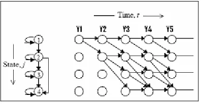
Y=y1,y2,y3…yT via a state sequence of length T, as a state only emits one observation at

each time t. The set of all such state sequences can be represented as routes through the

state-time trellis shown in Figure 2.2. The (j,t)th node (a state within the trellis) corresponds to the hypothesis that observation Yt was generated by state j. Two nodes

(i,t-1) and (j,t) are connected if and only if aij > 0.

Figure 2.2 - Hidden Markov Model showing the finite state machine for the HMM (left), the Observation sequence (top),and all possible routes through the trellis

As described above, we compute P(W|Y) by first computing P(Y|W). Given a state

sequence Q=q1 q2…qT, where the state at time t is qt, the joint probability, given a model

W, of state sequence Q and observation sequence Y is given by:

P(Y,Q|W) = b1(y1)

∏

= T t 2

aqt-1qtbqt(yt) (2.2)

Assuming the HMM is in state 1 at time t = 1, P(Y,Q|W) is the sum of all possible routes

(24)

P(Y|W) =

∑

allQ

P(Y,Q|W) (2.3)

In practice, the probability P(Y|W) is approximated by the probability associated with the

state sequence which maximizes P(Y,Q|W). This probability is computed efficiently

using Viterbi decoding. Firstly, we define the value δt (j), which is the maximum

probability that the HMM is in state j at time t. It is equal to the probability of the most

likely partial state sequence Q=q1 q2…. qt, which emits observation sequence

Y=y1,y2,y3…, and which ends in state j:

δt(j) =

qt q

q1max, 2... P(q1,q2…qt ; qt = j ; y1,y2…yt|W) (2.4)

It follows from Equation 2.2 and 2.4 that the value of δt(j) can be computed recursively as

follows:

δt(j) =

N i≤ ≤

1

max [ δt-1(i)aij].bj(yt) (2.5)

where i is the previous state (i.e. at time t-1). This value determines the most likely

predecessor state ψ t(j), for the current state j at time t, given by:

ψt(j) =

N i≤ ≤

1

max

arg [ δt-1(i)aij] (2.6)

At the end of the observation sequence, we backtrack through the most likely predecessor

states in order to find the most likely state sequence. Each utterance has an HMM

representing it, and so this sequence not only describes the most likely route through a

particular HMM, but by concatenation provides the most likely sequence of HMMs, and

hence the most likely sequence of words or sub-word units uttered.

Each node in the trellis must evaluate Equation 2.5 and Equation 2.6. This

(25)

observation probability bj(yt) to produce the result. After a number of stages of

multiplying probabilities in this way, the result is likely to be very small. In addition,

without some scaling method, it demands a large dynamic range of floating point

numbers, and implementing floating point multiplication requires more resources than for

fixed point. A convenient alternative is therefore to perform all calculations in the log

domain[10]. This converts all multiplications to additions, and narrows the dynamic

range. Hence Equation 2.5 becomes

δt(j) =

N i≤ ≤

1

max [ δt-1(i) +log aij] +log [bj(yt)] (2.7)

The result of these changes means that a node can have the structure shown in Figure 2.3.

The figure highlights the fact that each node is dependent only on the outputs of nodes at

time t-1, hence all nodes in all HMMs at time t can perform their calculations in parallel.

The way in which this can be implemented is to deal with an entire column of nodes of

the trellis in parallel.

(26)

Figure 2.4 - Decoder structure showing forward computation and backtracking

As the speech data comes in as a stream, we can only deal with one observation vector at

a time, and so we only need to implement one column of the trellis (In actuality,

implementing the entire trellis is area heavy and unnecessary as will be seen later. Instead

an optimum number of ‘node units’ are designed so that each unit will update a set

number of nodes). The new data values (observation vector yt and maximal path

probabilities δt-1(j)) pass through the column, and the resulting δt values are latched, ready

to be used as the new inputs to the column when the next observation data appears.

Each node outputs its most likely predecessor state yt(j), which is stored in a

sequential buffer external to the nodes. When the current observation sequence reaches

its end at time T, a sequencer module reads the most likely final state from the buffer,

chosen according to the highest value of δT(j). It then uses this as a pointer to the

collection of penultimate states to find the most likely state at time T-1, and continues

with backtracking in this way until the start of the buffer is reached. As the resulting state

sequence will be produced in reverse, it is stored in a sequencer until the backtracking is

complete, before being output. This state sequence reveals which HMMs have been

traversed, and hence which words or sub-word units have been uttered. This information

(27)

2.1.2 Phones & Triphones[11,12,13,14]

Equation 2.1 needs the quantity P(Y|W), the probability of an acoustic vector sequence Y

given a word sequence W to find the most probable word sequence. A simplistic

approach to achieve this would be to obtain several samples of each possible word

sequence, convert each sample to the corresponding acoustic vector sequence and

compute a statistical similarity metric for the given acoustic vector sequence Y to the set

of known samples. For large vocabulary speech recognition this is not feasible because

the set of possible word sequences is very large. Instead words may be represented as

sequences of basic sounds. Knowing the statistical correspondence between the basic

sounds and acoustic vectors, the required probability can be computed. The basic sounds

from which word pronunciations can be composed are known as phones or phonemes.

Approximately 50 phones may be used to pronounce any word in the English language.

For example, the sentence ‘This is speech’ is represented as ‘th ih s ih z s p iy ch’.

While phones are an excellent means of encoding word pronunciation, they are

less than ideal for recognizing speech. The mechanical limits of the human vocal

apparatus leads to co-articulation effects where the beginning and end of a phone are

modified by the preceding and succeeding phones. Recognizing multiple phone units in

context tends to be more accurate than recognizing individual phones. Current speech

recognition systems deal with three-tuples of phones called triphones. It is customary to

denote triphones as left context-current phone+right context. For example ‘th-ih+s’ is a

triphone that represents the context of the ‘ih’ phone in the word ‘this’. The final ‘ch’

phone in dissertation can be modeled with a cross-word triphone whose right context is

(28)

phone that denotes silence. Though there are approximately 50x50x50 = 125000 possible

triphones, only about 60,000 actually occur in English.

The front-end processes every 10ms data input and extracts relevant features that

will enable the recognition process. This involves converting every 10ms of speech into a

39-element vector, that has statistical information about itself (each element having

means, variances, mixture weights and scale factors). This then needs to be compared

using some distance measure to every triphone phone model and the observation output

probability for this input was obtained.

Initial HMM recognizers used discrete OPFs and sub-vector quantized (VQ)

models, which are easy to compute. The acquired acoustic vector was replaced by the

index of the closest codebook vector, and OPFs were just look-up tables containing the

VQ index probabilities. While this is computationally efficient, the discretization of

observation probability leads to excessive quantization error and thereby poor recognition

accuracy. To obtain better accuracy, modern systems use a continuous probability density

function and the common choice is a multivariate mixture Gaussian in which case the

computation may be represented as [8]:

∑

∏

= = = ⎟ ⎟ ⎠ ⎞ ⎜ ⎜ ⎝ ⎛ − − = M m N n jm jm t N n jm D m t j n n n y n w y b

1 1 2

2 1 2 2 / [ ] ]) [ ] [ ( 2 1 exp ] [ ) 2 ( ) ( σ µ σ π (2.8)

Here yt is the input vector, µjm and σjm represent the mean and standard deviation of the

multivariate Gaussian, wm is the mixture weight, m is the no. of mixtures and n is the no.

of feature vectors. The term before the exponent does not depend on the input and can be

(29)

2.8 and reduces the exponent calculation to simple multiplications. Performing these

modifications, Equation 2.8 reduces to

∑ ∑

= = × − = M m N n im jm t im t

j y c y n n V n

b

1 1

2 _[ _]

]) [ ] [ ( ) (

log µ (2.9)

Cim being the final mixture weight and Vim being the variance. The HUB4 speech

database which was considered for this research chose the values of M and N to be 8 and

39 respectively. The outer term represents an addition in the log domain. Every triphone

model would require pre-training which means that the number of parameters to be

estimated is about 60000 x (39x8x2+8) = 11.37 million parameters. The training data

usually available is insufficient to estimate so many parameters. The usual solution is to

cluster together HMM states and share a probability density function among several

states (Figure 2.6). Systems using such clustered probability density functions are called

semi-continuous or tied-mixture systems. Groups of states that are tied together are called

‘senones’. The total number of senones in the English Language ranges between 4000

and 6000.

The utterance hierarchy for the word ‘HI’ is shown in Figure 2.5. Each triphone is

represented by a 4 state HMM. Only the first 3 states are emitting states (i.e., they can

produce an observation vector yt). The last state is a null state. The overall effect is that of

combining all the triphone HMMs by adding null transitions between the final states of

one triphone HMM to the initial state of its successor. To model continuous speech, null

(30)

sil-hh+ay hh-ay+sil

Figure 2.5 - HMM for word ‘HI’, with phones ‘hh’&’ay, and triphones ‘sil-hh+ay’&‘hh-ay+sil’. Each HMM has 3 emitting senone states (striped oval) and one nullstate (plain oval).

Figure 2.6 - State-tying[7]

The viterbi search is modeled as a lexical tree search[15,16]. The roots of the tree

correspond to the set of all triphones that start any word in the dictionary. Each node in

the tree points to the next triphone in the expanded pronunciation of a word etc.

Triphones that occur at the end of a word are specially marked so that a language model

may be consulted at those points. Thus the lexical tree is a multi-rooted tree where each

node points to an HMM and a successor node. In the case of word exit triphones there are b1(yt) bb2(yt) 3(yt)

a00

a01 a11

a12 a22

a23

b1(yt) bb2(yt) 3(yt) a00

a01 a11

a12 a22

(31)

applied successively to the HMMs and the probability that the HMM generated that

vector is noted. Transitions are made in each step to successor nodes. On reaching a word

exit triphone, the state sequence history is consulted to find the word that has been

recognized. The last n words (usually n=3) are checked against a language model for

further analysis. Acoustic vectors are evaluated successively and on evaluating an HMM

for the current vector, if the HMM generates a probability above a certain threshold, the

successors of the HMM will be evaluated in the next time step. Thus there is always a list

of currently active HMMs/lexical tree nodes and a list of nodes that will be active next.

This combination of the Viterbi search combined with pruning techniques (comparing

with threshold) is known as the Viterbi Beam Search[17-20]. Pruning prevents

uncontrolled generation and maintenance of nodes with time by deactivating

low-probability paths.

2.2 Language modeling

The introduction of a language model to the speech recognition unit increases accuracy of

the recognition hypothesis [21-23]. It helps introduce additional biases to the several

alternate similar words that the acoustic model recognizes and cannot choose between.

This also helps in the quick pruning of improbable paths and the unnecessary explosion

of node generation. All state-of-the-art speech recognition systems implement a language

model in one form or the other, and so it is necessary to study the language model in

order to build a system that is commercially competitive.

N-gram models [24,25] that predict the probability of a word sequence (in other

(32)

and common approach. They encode simultaneously the syntax, semantics and

pragmatics and they concentrate on local dependencies. They are thus extremely effective

for languages like English in which word order is important and the strongest contextual

effects come from near neighbors. They also have the distinct advantage of being easy to

train. N-grams can be trained automatically from a large corpus of text.

The complexity of the modeling increases logarithmically with the size of the

vocabulary V (the complexity for an N-gram vocabulary will be V^N). Large values of N

lead to complexities both in the viterbi decoding stage as well as the training stage, where

sparse training data leads to incorrect parameter estimation. This may even have a

deteriorating effect on the recognition accuracy. Thus a modest value of 3 is chosen, and

this has proven to be sufficient in systems like Sphinx and HTK. Such models are called

trigrams. A trigram model may be trained using the following equation [26]:

) 2 , 1 ( ) 3 , 2 , 1 ( ) 2 , 1 | 3 ( w w F w w w F w w w

P = (2.10)

Here, F(w1,w2,w3) refers to the frequency of occurrence of the trigram (w1,w2,w3) in the

training text and F(w1,w2) refers to the frequency of occurrence of the bigram (w1,w2).

In practice, for a large vocabulary all possible trigrams will not be present in the training

corpus. In that case bigram or unigram probabilities are used in the place of trigram

probabilities after reducing the probability by a back-off weight, which accounts for the

fact that the next higher N-gram has not been seen and therefore has a lower chance of

occurring [27].

A typical example of the use of a language model is shown in Figure 2.7. The

(33)

contention in recognizing the phrase ‘I the’, instead of the actual phrase ‘I need the’.

With the language model, the improbable paths are pruned out leading to a good

(34)

Figure 2.7 - Use of Language model

(a) Shows the four words ‘I’,’Need’,’The’ and ‘on’, on the y-axis and the paths that the different hypotheses take as the input phones ‘aa n iy dh ax’ come in.

(b) Shows the word models for the 4 words.

(c) Shows the Bigram Probabilities obtained from the Brown Switchboard Corpus (d) Shows the path probabilities without the use of the language model.

(35)

(a) (b)

Bigram Probabilities

# Need 0.00018

# The 0.016

# On 0.00077

# I 0.079

I need 0.0016

I the 0.00018

I on 0.000047

I I 0.039

on need 0.000055

on the 0.094

on on 0.0031

on I 0.00085

need need 0.000047

need the 0.012

need on 0.000047

need I 0.000016

the need 0.00051

the the 0.0099

the on 0.00022

the I 0.00051

(36)

(d) (e) aa ay aa n dh n iy ax n iy d I on the need

aa n iy dh ax

2.6e-6x1=2.6e-6 .20x.079=.0016 .0016x.0016=2.6e-6 2.6e-6x.012x.92=2.9e-8 2.9e-8x.77=2.2e-8 .20x.079=.0016 .0016x.00018x.08=2.3e-8 2.3e-8x.12=2.8e-9 1x.00077=.00077 .00077x1=.00077 .00077x0=0 2.8e-9x0=0 aa ay aa n dh n iy ax n iy d I on the need

aa n iy dh ax

(37)

CHAPTER 3 Related Work

Several speech recognition applications have been developed in the industry and sold as

commercial products. Several speech applications and training kits are also available

from universities that are mainly oriented at speech research. Speech Recognition is

inherently a computationally demanding task and hence software solutions running on a

general-purpose processor are not good at real-time speech recognition. These systems

are not particularly designed keeping underlying architecture in mind and hence end up

squeezing all available resources of the processor. Some of the systems available are

discussed below.

3.1 Commercially Available Systems

Commercially available software systems are IBM’s ViaVoice and Dragon Systems

Dragon Naturally Speaking, claim to be able to support between 10k and 150k

vocabulary sizes. They are speaker independent though some amount of training is

encouraged. The systems can support multiple languages and report a >95% accuracy.

They are however slow and sensitive requiring the user to speak slowly and

(38)

output. These also take up a large amount of the CPU processing power effectively

blocking it from doing other tasks and also consume a large amount of power.

Considering the ‘always on’ nature of speech, these software at best work as a

‘speech-to-text’ solution used for small periods of time for very specialized functions, and are not

the best step towards making speech a general user interface.

Since a lot of the research has been done with a product in mind, the systems used

at Dragon [28-30] usually require a lot less resources than other research systems. For

instance, while most systems were using a 10ms frame size, Dragon decided to use a

coarser sampling of 20ms frame sizes. While most systems use 32-bit floating point

formats for their input features, Dragon used 8-bit fixed-point parameters. To reduce the

resource requirements even more, the commercial version applies automatic vocabulary

switching to restrict the search space.

The IBM speech recognition system differs form other competing systems by the

early use of a rank-based approach for the computation of observation probabilities that

allows avoiding certain search problems related to extreme probability values. The search

strategy is a combination of an A*[31,32] with a time-synchronous Viterbi search (the so

called ‘envelope search’) and is therefore difficult to compare to the fully

time-synchronous search of other systems. Other features that made this system substantially

different from its competitors include that during the first recognition pass the usual

mixture of Gaussian probabilities were replaced by a probability derived from the rank of

the models score [33-36]. The system has a recognition vocabulary of 65,000 words.

A version of ViaVoice is also available for embedded processors and mobile

(39)

on template recognition rather than speech processing. It has a maximum of 16k

vocabulary and maintains a dynamically swappable 4,000 word phonetic flat list. It is

speaker independent but has small database support. This system requires several minutes

of read speech to adapt to a new user.

The AT&T Watson speech recognition engine [27,37-39] is a software

implementation of the AT&T voice processing technology. It uses a gender based

triphone model and a 5-gram language model. The recognition takes place in 2 phases –

the first pass does the phone recognition, word recognition and builds the word lattice;

the second pass rescores the word graph.

Microsoft’s Whisper [31,40,41] is an adaptation of CMU’s SPHINX and

incorporates speaker adaptation and noise cancellation. The acoustic models are

compressed and hence Whisper claims to be memory efficient. The software supports a

60,000-word vocabulary with the ability to add new words. It works with any Windows

application and has two specialized applications for use in Windows - "Dictation Pad"

provides enhanced dictation features while "IntelliSense" converts spoken numbers and

times automatically.

SRI’s DECIPHER [42-44] is another HMM-based system that uses multi-pass

time synchronous Viterbi decoding. A first forward-backward pass generates

word-lattices using a 60,000-word bigram language model and context-dependent hidden

Markov models. Only within-word context dependent models were used in the first pass.

The Gaussian computation was sped up using vector quantization and Gaussian shortlists.

The second pass performed a forward-backward N-best search on the word-lattices using

(40)

expensive acoustic and language models. Most of the development effort went into the

reduction of the error rate, and only little research was reported on means for achieving

real time recognition.

SRI‘s ‘Phraselator’ [45] is a template based phrase recognition and translation

system. The Phraselator is a handheld, wireless computer used to translate more than

1,000 spoken English phrases into languages such as Arabic and Pashto. This is again a

lookup engine rather than a recognition engine.

Several smaller companies have developed IC’s for small end applications like

voice-responsive toys and voice dialers [46-50].

3.2 Research Systems

SPHINX speech recognition systems [4,13,20,51-56] are CMU’s state-of-the-art large

vocabulary speech recognition systems. They are semi continuous HMM based [13]

systems and use state-tied triphone models. It uses scaled integer observation probability

computation. Decoding is done in 2 phases with a first pass viterbi decoding done to

reduce the search space and a second pass A* algorithm to combine the results of the first

pass and the language models. Beam searches and various pruning strategies ate used to

reduce the computations and prune paths quickly. However the CMU-SPHINX system

uses an extraordinary amount of power while running on desktops and the power required

is prohibitive for mobile applications. The SPHINX–IV system is CMU’s speech

recognition system for the mobile domain. It however supports a much lower vocabulary

(41)

Cambridge University’s ABBOT system differs significantly from other systems

by being the only neural net driven system used in large-scale evaluations [57-59]. It is

also among the few systems to use a stack decoder rather than a time synchronous Viterbi

algorithm for the search process. The ABBOT system supports a 65,000-word

vocabulary. The recognition speed for this system in the evaluation was estimated to

about 60 times slower than real time on a 170MHz UltraSparc.

Cambridge University’s HTK system was the best recognizer in the 1994 LVCSR

evaluation with a word error rate of only 10.5% [60,61]. All promising algorithms such

as quinphone models, cross-word models, 4-gram language models and unsupervised

speaker adaptation were applied to this system. Considerable effort was also invested in

the pronunciation dictionaries. The commercial cousin of this system ‘Entropics’ is more

stable and more toolkit-oriented.

SONIC [62] is a toolkit for enabling research and development of new algorithms

for continuous speech recognition. The system uses HMM acoustic models and a

two-pass search strategy. Model-based adaptation methods such as Maximum Likelihood

Linear Regression (MLLR), Structured MAP Linear Regressions as well as

feature-based adaptation methods such as Vocal Tract Length Normalization, cepstral mean &

variance normalization, and Constrained MLLR are implemented [63].

3.3 Implementations on general-purpose processors

Several approaches have been taken towards finding solutions to the problems of speed,

accuracy and power consumption. Research has been traditionally geared towards

(42)

largely ignored. Even the yearly HUB speech recognition evaluation reports typically

emphasize improvements in recognition accuracy and mention improvements in

performance as a multiple of “slow down over real-time” [64, 65].

Binu [4] used rapid semi-automatic generation of low-power high performance

VLIW processors for the perception domain. Energy efficiency was primarily achieved

by minimizing communication and activity using complier-controlled fine-grain clock

gating. Ravishanker’s research improved the performance of the Sphinx speech

recognition system by trading off accuracy in a computationally intensive phase for faster

run time and then recovered the lost accuracy by doing additional processing in a

computationally cheaper phase of the application [52]. This research also reduced the

memory footprint of speech recognition by using a disk based language model cached in

memory by the software. Agram, Burger and Keckler characterized the Sphinx II speech

recognition system in a manner useful for computer architects [66]. They focused on ILP

as well as memory system characteristics including cache hit rates and block sizes and

concluded that available ILP was low. They compared the characteristics of the Sphinx II

system with those of Spec benchmarks and also hinted at the possibilities and problems

associated with exploiting thread level parallelism.

Intel ICRC lab researchers executed the Intel speech recognition system on

several versions of the x86 processor [67]. The study focused on the run time and size of

the working set, and the language was Mandarin Chinese. They reported a decrease in

ILP with increased clock rate. IPC decreased from between 1 and 1.2 at 500MHz to .4 at

1.5 GHz. Obviously increasing clock rate is not the solution to improving speech

(43)

but a detailed explanation was not provided. The ICRC speech system is not publicly

available, and details of the ICRC workload are not available.

3.4 Hardware solutions

A common approach to finding a solution to the problems of speed, accuracy and power

consumption is to build hardware accelerators to speed up parts of the speech recognition

process or build a complete hardware speech recognition system.

An earlier attempt to accelerate speech recognition may be found in the work of

Anantharaman and Bisiani [68], who presented a multi-processor architecture as well as a

custom architecture for improving the beam search algorithm used in the CMU

distributed speech recognition system. The paper also describes the design process of the

custom architectures and presents a number of ideas on the automatic design of custom

systems for data dependent computations.

Researchers at the Norwegian University of Science and Technology designed a

custom probability density function (PDF) coprocessor in a 0.8µ CMOS process that

could accelerate the computation of Gaussian observation probabilities in a hidden

Markov model based speech recognizer [69]. This research concluded that memory

bandwidth was a limiting factor for Gaussian computation. They approached the memory

bandwidth problem by using a new fixed point representation called dynamical circular

fixed-point format which reduced the memory bandwidth in half. The PDF coprocessor

could evaluate 40,000 39-element Gaussian components in real time using this format at

154 MHz consuming 853 mW of power. The workload has worsened by a factor of 15.3

(44)

current systems that fixed point does not meet the required range of generated

probabilities necessary for high accuracy speech recognition.

Sergiu.et.al[70] implemented a low power speech recognition system that

performs real-time speech recognition. This is a complete design that has its own

language and acoustic model. It exploits parallelism existing in speech recognition

algorithm with multiple Processing Elements (PE). Parallel execution helps in reducing

clock frequency resulting in reduced power usage. Dynamic loading of speech models is

used for changing language grammar and retraining, while reprogramming is used to

support evolution of recognition algorithms. The focus on small sets of words (at one

time) reduces the complexity, cost and power consumption. The recognizer is extremely

flexible and can support multiple languages or dialects with speaker-independent

recognition. The average power dissipation for the logic part of the decoder was about

5.125mW in the 0.18µm process, and area of the design was about 2.5mm2. Evaluations demonstrate an order of magnitude improvement in power compared with optimized

recognition software running on a low-power embedded general-purpose processor of the

same technology and of similar capabilities. The design however is only good for a very

small vocabulary and is phoneme based, therefore it is not good for real life use.

Binu [71] improved memory bandwidth on the SPHINX –III systems by using a

blocking scheme whereby a single retrieved set of variances, means, weights and scales

were used to calculate the observation probabilities for 10 frames. A special-purpose

accelerator for the dominant Gaussian probability phase was developed for a 0.25µ

CMOS process. Area, power and bandwidth efficiency are achieved by reducing the

(45)

restructuring the computation, and sharing memory bandwidth. The accelerator improves

performance of aPentium 4 (.13µ) system running the SPHINX – III system by a factor

of 2, while simultaneously improving on the energy consumption by 2 orders of

magnitude. The Gaussian accelerator consumed 1.8 watts while the Pentium 4 consumed

52.3 watts during Gaussian computation, representing an improvement of 29 fold.

Researchers at the Tsinghua University developed a single chip speech

recognition system based on an 8051 microcontroller core [72]. The chip was designed

based on the SOC (system on chip) philosophy and an 8-bit MCU, RAM, ROM,

ADC/DAC, PWM, I/O ports and other peripheral circuits were all embedded in it.

Software modules including control/communication, speech coding and speech

recognition algorithms were implemented in an 8051 compatible microcontroller core,

resulting in the extremely low cost of the chip. The speech recognition adopted the

template matching technique, and recognized up to 20 phrases with an average length of

1 second and a recognition accuracy reaching more than 95% with the background SNR

above 10 dB. The design operated at 40 MHz and consumed 60mW of power.

Borgatti et.al [73] developed a low-power, low-voltage speech processing

intended to be used in remote speech recognition applications where feature extraction is

performed on terminal and high-complexity recognition tasks are moved to a remote

server accessed through a radio link. Power optimization of portable terminals featuring

speech recognition was pursued by partitioning speech recognition complexity between

on-terminal circuitry and remote hosts. The proposed system was based on a CMOS

feature extraction chip for speech recognition that computed 15 cepstrum parameters,

(46)

achieved. Processing relied on a novel feature extraction algorithm using 1-bit A/D

conversion of the input speech signal. The chip was implemented as a gate array in a

standard 0.5-µm, three-metal CMOS technology. Recognition rates above 98% were

achieved in isolated-word speech recognition tasks.

LOGOS [74] is a real time hardware speech recognition system that uses both

parallel and pipelined processing techniques, matching up to several hundred words from

a previously stored vocabulary of whole word "templates" in real time. An efficient

single pass dynamic programming algorithm is used to find the sequence of templates

that best represents the input. Continuous recognition is achieved using a trace back

technique on partial recognition results. Vargas et.al [75] proposed a novel HW/SW

co-design with redundancy techniques to implement a speech recognition system. Special

attention needs to be taken when partitioning digital signal processing algorithms into

hardware and software parts. The design methodology in this work partitions the HW and

SW parts in such a way as to boost system performance while maintaining low area

overhead. The proposed approach is called the "speech recognition-oriented HW/SW

partitioning and fault-tolerant design" approach (or simply SCORPION approach). Other

VLSI-based designs[76,77] for HMM speech recognition also exist.

The most recent research effort towards a hardware solution to the speech

recognition problem is CMU’s ‘Moving Speech Recognition from Software to Silicon:

the In Silico Vox’ research project [3,78]. The project is looking at both an FPGA

approach as well as an ASIC solution to building massively parallel, energy efficient

speech chips that will attain high performance. The FPGA approach plans to use a Xilinx

(47)

design will operate about 2.3 times slower than real-time due to memory bandwidth

constraints. The ASIC implementation will be designed to recognize about 5000 words,

operating at about 6 times faster than real time requirements. The overall size of the chip

is estimated to be about 10mm2. The latest publication [79] from this group indicates successful design of an ASIC implementation that recognizes speech at .6xRT (real time),

and runs at 125MHz. Hardware prototyping on a Xilinx XC2VP30 FPGA, using a Xilinx

XUP development board has also been completed. The prototype recognizes about 1000

words at roughly 2xRT. No power readings were reported.

The use of reconfigurable logic and FPGA devices is another common approach

to the speech recognition problem [6, 80]. Techniques vary from power aware mapping

of designs onto commercially available FPGA devices to hybrid methods where

specialized function blocks are embedded into a reconfigurable logic array [81,82]. The

inherent reconfigurability of FPGAs provides a level of specialization while retaining

significant generality. FPGAs, however, have a significant disadvantage both in

performance and power when compared to either ASIC or CPU logic functions.

Melnikoff et. tried to exploit the parallel nature of the algorithm to implement the

decoder part of the speech recognition system onto an FPGA[83]. The question of how to

deal with limited resources, by reconfiguration or otherwise, was also addressed. A later

publication [84] indicated that the design was implemented on a Xilinx Virtex XCV1000

FPGA, sitting on Celoxica’s RC1000-PP development board. The design occupied 5,590

of the XCV1000’s slices, equal to 45%, and ran at 44 MHz. The correctness values (less

than 60%) are clearly much lower than those found in commercial speech recognition

(48)

Vargas et a.[85] used a new approach by which the Viterbi algorithm is built in

with the HMM structure. The probabilistic state machines run as parallel processes and

the entire system is built as a hardware/software co-design. The design is intended for

isolated word recognition, and runs 500 faster than classic implementations.

3.5 Digital Signal Processing solutions

It is common practice to use special DSP techniques to try to reduce the number of

operations performed and speed up the algorithm. Bocchieri [86] used vector quantization

of the input vector to identify a subset of gaussian neighbors so that only a smaller subset

of likelihood computations needed to be calculated with only a small loss in accuracy.

In [87], the authors reduced the word error rate for speaker-independent continuous

speech recognition by modeling subphonetic events with HMM states and treating the

state in phonetic hidden Markov models as the basic subphonetic unit. Lee et al [88]

used context-independent models for selection and back off of corresponding triphone

models. Another study [89] used lookahead HMMs and frame skipping to skip the

gaussian calculation for frames that do not show significant change from the previous

frame(s). Much effort has been spent on optimizing the computation of likelihood for all

tied triphone states [90-94]. The authors in [95] categorize the different schemes into 4

layers, and described how the different layers can interact with each other and

compliment each other. These techniques and their relevance are discussed further in

(49)

CHAPTER 4 System Architecture

The Speech Recognition System can be separated into 3 separate units – the Front-End,

the Gaussian Estimator, and finally, the Viterbi Decoder. Figure 4.1 shows the overview

of the system. The Front end processes the spoken input and provides mel-frequency

cepstral coefficients (MFCCs) of the input data to the Gaussian Estimator. The Gaussian

Estimator then uses this input along with the acoustic models to provide the

phone/senone scores. The Viterbi Decoder uses this information along with the language

models to calculate the state transitions and word-to-word transition probabilities and

search for the most likely sequence of words.

Figure 4.1 - System Overview

Profiling of the speech recognition process shows that system spends approximately

.89%, 49.8% and 49.3% [4] of its compute cycles in the Front-End, Gaussian Estimation Front

End

Phone Decode Stage (Gaussian Estimator)

Acoustic Models

Language Model Word Decode

Stage (Viterbi Decoder) Phone

Lattice Feature

Vectors Spoken

(50)

and Viterbi Decoding Stages respectively. Fortunately, both the compute heavy stages are

extremely parallelizable, making them ideal candidates for translation into hardware.

In our implementation we used a 4 state HMM model that was the most common

choice among speech recognition systems. The Gaussian Estimator unit was modeled as a

32-bit unit though 20-bit implementations have proven to be sufficient [101]. This was so

that we would be able to work with standard 32-bit acoustic scores, and optimize down

once the initial implementation was complete.

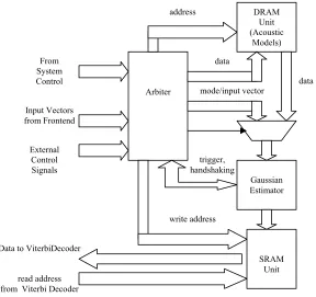
Figure 4.2 shows the overview of the implementation of the complete system. The

system consists of a ‘Gaussian Estimator’, a ‘Viterbi Decoder’, a ‘System Control’, an

‘Arbiter’, three DRAMS and an SRAM. The system acts like a co-processor that

interfaces with a host processor. The front-end will be implemented on the host processor

providing inputs to our co-processor at 16kbps. The Arbiter acts as control to the

Gaussian Estimator and also directs the inputs from the front-end to it. Initially it was

envisioned that the Arbiter would be used to control any feedback from the Viterbi

Decoder that we may implement. The final system does not contain feedback. The

Arbiter is also responsible for initializing the DRAM Unit (with the Acoustic Models).

The Gaussian Estimator updates and places the phone/senone scores in the SRAM every

frame. The Viterbi Decoder accesses these scores as well as other data in the two DRAM

units to complete the process, and place the outputs in the form of a sequence of word

indexes on the ‘output’ bus. The Viterbi Decoder is an extremely self-sufficient unit

requiring minimal external control. System Control acts as control unit for the entire

system and is also responsible for initializing DRAM UNIT –1 and DRAM UNIT –2

(51)

Figure 4.2 - System Implementation Overview

The different parts of the system are discussed in detail in the following chapters. We use

this chapter to also briefly describe the Front End. This part of the system is not

implemented in hardware as it is responsible for less that 1% of the total computation

workload and can easily be done by a host processor

4.1 Front-End

Even though the front end only occupies less than 1% of the compute time on speech

systems, it is very important for two reasons – (a) The front-end is responsible for

generating a good smooth spectral estimate of the incoming speech waveform and is

directly responsible for obtaining good output observation probability estimates (b)

Understanding acoustic vectors is a crucial prerequisite to understanding the operation of

the acoustic model. The Front-End is not dealt with in detail in this research, and the

implementation (which is almost standardized at this point) is obtained from [102]. The

overview is shown in Figure 4.3.

Viterbi Decoder DRAM UNIT - 1

SRAM UNIT

Gaussian Estimator

DRAM UNIT Acoustic

Models Arbiter

System Control

DRAM UNIT - 2

Input Vectors from Front End Control

Signals Control

(52)

Figure 4.3 - Front-End [102]

The human vocal apparatus has mechanical limitations that prevent rapid changes to

sound generated by the vocal tract. Thus, speech signal are considered to be

quasi-stationary, i.e., stationary in short time intervals (typically 5-20 ms), during which the

spectral characteristics are relative constant. DSP techniques may be used to summarize

the spectral characteristics of a speech signal into a sequence of acoustic observation

vectors, with a single vector representing about 10 ms of speech.

The front-end segments the signal into blocks and makes a smooth spectral

estimate for each block. The (constant) length of the blocks is typically chosen to be 10

ms, and the blocks are overlapped in time to give a longer analysis window of 25 ms

Hardware Implementation of a Low Power Speech Recognition System

ABSTRACT

DEDICATION

BIOGRAPHY

ACKNOWLEDGEMENTS

TABLE OF CONTENTS

LIST OF TABLES

LIST OF FIGURES

CHAPTER 1

Introduction

1.1

The Problem

1.2 The Solution

1.3 Organization of the Dissertation

CHAPTER 2

Background

2.1 Acoustic Modeling

2.1.1 A brief overview of speech recognition and HMMs [1, 4, 6, 7, 8, 9]

∏

∑

2.1.2 Phones & Triphones[11,12,13,14]

∑

∑

∏

∑ ∑

2.2 Language modeling

CHAPTER 3

Related Work

3.1 Commercially Available Systems

3.2 Research Systems

3.3 Implementations on general-purpose processors

3.4 Hardware solutions

3.5 Digital Signal Processing solutions

CHAPTER 4

System Architecture

4.1 Front-End