High Temperature Graphite Simulations using Molecular Dynamics

Abstract

HEHR, BRIAN DOUGLAS. High Temperature Graphite Simulations using Molecular Dynamics. (Under the direction of Ayman I. Hawari).

Graphite, a major structural and moderator material in the proposed Generation IV reactor roadmap, is expected to experience irradiation at temperatures up to 1800 K. In this study, molecular dynamics (MD) is employed to investigate the physical properties of graphite from 0 K to 1800 K. MD applies the classical laws of physics to simulate atomistic-level behavior, and from the observed microscopic data, macroscopic properties may be surmised.

For the purposes of this study, a graphite-specific MD code was created and

benchmarked against high temperature graphite data. Modifications were introduced into the interatomic potential function as needed to fit experimental measurements. Graphite-specific modifications include a plane-by-plane center of mass velocity correction, an additional potential energy cutoff function for out-of-plane displacements, and temperature-dependent parameterization of the potential function. These adjustments were fitted to high temperature measurements of thermal expansion and mean squared displacement.

High Temperature Graphite Simulations

Using Molecular Dynamics

by

Brian D. Hehr

A thesis submitted to the Graduate Faculty of North Carolina

State University in partial fulfillment of the requirements for

the Degree of Master of Science

Nuclear Engineering

Raleigh, NC

2007

Approved by:

________________ ________________

Dr. Bernard W. Wehring

Dr. K. L. Murty

______________________

Dr. Ayman I. Hawari,

ii

Biography

Brian Douglas Hehr was born in Reading, Pennsylvania on December 21, 1981 to parents Steven and Brenda Hehr. At the age of 3, Brian and his family moved to the vicinity of Charlotte, NC. Brian graduated from Sun Valley High School in 2000 and subsequently enrolled at North Carolina State University, where he graduated summa cum laude with dual

B.S. degrees in physics and nuclear engineering. During his undergraduate studies, Brian participated in four summer internships – two at the Clariant Corporation headquarters in Charlotte and two at Los Alamos National Laboratory in New Mexico.

Immediately following graduation, Brian began working with Dr. Ayman Hawari of North Carolina State University on atomistic graphite simulations. During his first year of graduate study, Brian traveled to Tokyo to marry his long-time pen pal Atsuko Miyamoto, who has since become a permanent resident of the U.S.

iii

Acknowledgements

I would like to offer my gratitude to Dr. Ayman Hawari, who originated the ideas behind this project and guided its subsequent development. I would additionally like to thank him for offering valuable input on papers and presentations that I composed during the course of my studies.

I would also like to extend my appreciation to Dr. Victor Gillette for setting aside many hours of his time to help guide me through the initial stages of the project, and for educating me about his homeland of Argentina.

Finally, I would like to recognize the Advanced Fuel Cycle Initiative of the US DOE Office of Nuclear Energy for their support via the AFCI / GNEP Fellowship Program. The University Research Alliance did a great job of administering fellowship funds diligently and responsively, and I’m very grateful for the opportunity afforded to me by the fellowship to visit Idaho National Laboratory and the DOE headquarters in Washington D.C. At both locations, I was highly impressed with the hospitality and enthusiasm of our hosts.

iv

Table of Contents

List of Tables

... vi

List of Figures

... vii

Chapter 1 Introduction

... 1

1.1 Introduction... 1

1.2 Generation IV Concept and the VHTR... 2

1.3 Relevance to Thermal Neutron Scattering... 4

1.4 Structure of Graphite... 5

1.5 Computational Techniques ... 7

1.6 History of MD... 8

Chapter 2 Basics of Molecular Dynamics

... 9

2.1 Introduction... 9

2.2 Finite Difference Method... 9

2.3 Predictor-Corrector ... 10

2.4 Periodic Boundary Conditions... 12

2.5 Ensembles ... 14

2.6 Initial Velocities... 14

2.7 Center of Mass Correction... 15

2.8 Velocity Rescaling... 16

2.9 Potential Energy Function... 17

2.9.1 Abell Formalism ... 18

2.9.2 Reactive Bond Order Potential (REBO) ... 21

Chapter 3 Motivation for a New Model

... 27

3.1 Graphite Structure... 27

3.2 Absolute Zero Fitting... 28

Chapter 4 Description of the NCSU MD Model

... 30

4.1 Introduction... 30

4.2 Thermal Bath ... 31

4.3 Interplanar spacing... 31

4.4 Center of Mass Correction... 32

4.5 Modifications to the Potential Function... 33

4.5.1 Anisotropic Cutoff ... 33

4.5.2 Pairwise Coefficients ... 35

Chapter 5 MD Results

... 36

5.1 Absolute Zero Properties ... 36

v

5.2.1 Potential Energy... 37

5.2.2 Standard Deviation in Temperature ... 38

5.3 High Temperature Physical Properties ... 40

5.3.1 Thermal Expansion ... 40

5.3.2 Mean Squared Displacement ... 48

5.3.3 Bond Length... 53

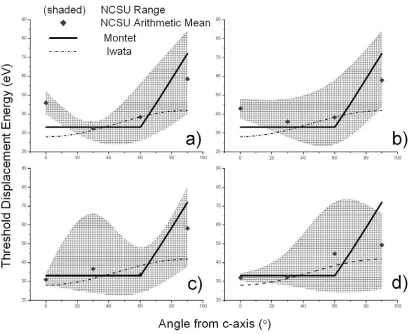
5.3.4 Radiation Damage & Threshold Displacement Energy... 56

Chapter 6 Conclusions and Future Work

... 61

6.1 Conclusions... 61

6.2 Future Work... 62

6.2.1 Cascade Collisions ... 62

6.2.2 Nuclear Grade Graphite ... 63

References

... 64

Appendix

... 66

Appendix A... 67

vi

List of Tables

vii

List of Figures

Fig. 1-1. Schematic of the proposed VHTR system ... 3

Fig. 1-2 The crystal structure of perfect graphite ... 6

Fig. 1-3 Sheets of pyrolytic graphite... 7

Fig. 2-1 Periodic Boundary Conditions. ... 13

Fig. 2-2 Transport phenomenon under PBC. . ... 13

Fig. 2-3 Potential energy of graphite at 0 K as computed using the REBO potential.. ... 26

Fig. 3-1 Profile of a simulated array of graphite using the REBO potential with fixed boundary atoms. ... 27

Fig. 3-2 Out-of-Plane MSD at 1200 K as computed using the published form of REBO.... 28

Fig. 3-3 MD calculation of thermal expansion using the published form of the REBO potential... 29

Fig. 4-1 Flowchart of the NCSU MD code... 30

Fig. 4-2 C/A Ratio for Graphite... 32

Fig. 4-3 Profile of the c-axis cutoff function, f_c'

( )

z,T .. ... 34

Fig. 5-1 Energy profile as a function of lattice parameter at 0K ... 37

Fig. 5-2 Mean potential energy vs. temperature. Comparison is made to the harmonic approximation. ... 38

Fig. 5-3 Comparison of the temperature fluctuations of a graphitic system as calculated from MD simulations (dots) and the derived theoretical model (solid curve)... 40

Fig. 5-4 Predicted C(T) up to 1800 K. ... 43

Fig. 5-5 Sigmoidal Fit to Estimated C(T) ... 44

Fig. 5-6 Attractive and repulsive coefficients of the modified REBO potential as a function of temperature, normalized to their (constant) published values. ... 45

Fig. 5-7 Effect of C(T) on Thermal Expansion... 45

Fig. 5-8 Average potential energy as a function of lattice parameter at: a) 300 K , b) 650 K , c) 900 K , d) 1200 K , e) 1520 K , and f) 1822 K using the temperature-adjusted REBO potential. ... 47

Fig. 5-9 Computations of the average potential energy at 1822 K, with error bars representing the standard error in the sample mean. ... 47

Fig. 5-10 Impact of C(T) on the interatomic potential energy curve... 48

Fig. 5-11 Representative MSD profile of a solid, liquid, and gas. [18]... 49

Fig. 5-12 Asymptotic convergence of the graphitic a-axis and c-axis MSD at 1200 K. ... 50

Fig. 5-13 In-plane and out-of-plane MSD as a function of temperature. ... 52

Fig. 5-14 Evolution of the minimum, maximum, and average interatomic bond length during the course of a 1500 K NCSU MD simulation... 54

Fig. 5-15 Increase in average interatomic distance (bond length) with temperature. A 2nd order polynomial fit is superimposed on the data... 54

1

Chapter 1

Introduction

1.1 Introduction

Graphite – in one form or another – has been a significant nuclear material ever since the inception of controlled fission in the 1930’s and 40’s. In fact, the world’s first functional nuclear reactor (referred to as Chicago Pile-1) contained piles of graphite blocks that slowed neutrons down to the thermal energy range. Graphite-moderated reactors have subsequently been constructed in several nations for research or power generation purposes.

While light water reactors (LWRs) presently dominate the realm of commercial nuclear power production, graphite remains one of the foremost candidate materials for use in the proposed Generation IV reactor designs. Its attractiveness lies in an almost unique combination of desirable properties, including:

• High mechanical strength • Large heat capacity

• Very high melting temperature

• Small cross section for neutron absorption • Relatively low density

2 in conjunction with experimental studies, provides an excellent array of tools for examining the behavior of graphite in a Generation IV type environment.

1.2 Generation IV Concept and the VHTR

The Generation IV initiative is a global partnership that aims to deploy a new generation of safe, economical, sustainable, and reliable reactors for the purpose of commercial energy generation. Presently, the vast majority of commercial reactors are water cooled and moderated, with power production taking place in a network of UO2 fuel assemblies. While these light water reactors (LWRs) have an excellent operating record, new advances have led to the conceptualization and initial design of several innovative reactor concepts, among which the Very High Temperature Reactor (VHTR) has figured prominently.

3 VHTR – is the potential coupling of the reactor system to an external thermochemical process for producing hydrogen gas, steel, or aluminum.

Fig. 1-1. Schematic of the proposed VHTR system including a coupled hydrogen production facility [1].

A number of factors lie behind the choice of graphite as the preferred moderator for the VHTR. First, in terms of the moderating figure of merit (FOM):

a s

FOM

Σ Σ

= ξ (1.1)

graphite’s FOM of 192 compares quite favorably against the FOM of 71 for light water. Here, Σs and Σa are the macroscopic scattering and absorption cross sections respectively

4 state moderator, graphite further performs the function of a structural material. This is made possible by its exceptionally high melting temperature of approximately 3700°C.

The static residence of graphite in the reactor core implies that radiation-induced defects will accumulate over time and may exert a significant impact of the properties of the moderator. In view of this fact, the present work focuses on the development of a high temperature molecular dynamics code for graphite and its application in performing an initial evaluation of defect formation at various temperatures between 300 K and 1800 K (up to the accident temperature of the VHTR).

1.3 Relevance to Thermal Neutron Scattering

In addition to the impact of neutron irradiation on the mechanical and physical properties of graphite, which is well documented in literature [2], there are reasons to believe that neutronic properties also can be affected. Because the introduction of vacancies and interstitials into the lattice structure perturbs the phonon frequency spectrum, the presence of these defects can impact neutron interactions in the thermal energy range – where phonon creation and annihilation processes contribute sizably to the scattering cross section [3]. The resulting change in the thermal neutron energy spectrum has implications in safety and criticality assessment of nuclear reactors.

5

( )

( )

(

S Q w S Q w

)

k k dE d d s incoh

cok , ,

' 4

1

2 _{v r}

σ σ

π

σ _{= +}

Ω (1.2) where k and k’ represent the magnitude of the wave vector of the incident and scattered neutron respectively, σ_coh is the bound atom coherent scattering cross section, σ_incoh is the bound atom incoherent scattering cross section, and S

( )

Qv,w is the scattering law in which

'

k k

Qr = r− r . The scattering law may be decomposed into two terms:

( ) ( ) ( )

Q w S Q w S Q w

S r, = _s r, + _d r, (1.3) where Ss is the self scattering law and Sd is the distinct scattering law. Of these two functions, the self scattering law is typically much simpler to calculate. Thus, the primary challenge lies in determining the distinct component or, alternatively, the total scattering law, from which Sd can be extracted via Eq. (1.3). Using the Van Hove formulation, the total scattering law may be written as:

( )

_{∫ ∫}

∞

( )

( ) ∞ − ∞ ∞ − − ⋅

= G r t e drdt

h w

Q

S r r iQrr wt r

r

, 2

1 ,

π (1.4) in whichG

( )

rr,t is the probability of finding the atom at position rrat time t. Since the atomic

positions are known exactly throughout the time evolution of an MD system, G

( )

rr,t is directly calculable in MD and the scattering law may be computed by taking the Fourier transform of G

( )

rr,t as in Eq. (1.4). This approach applies to both damaged and undamaged systems.

1.4 Structure of Graphite

6 to permit only Van der Waals interactions between atoms occupying different planes. Very strong covalent bonds exist within each plane, and the exceptionally large cohesive energy of 7.37 eV is primarily responsible for the high melting temperature of graphite. Conductivity is also dependent on crystallographic direction, with a high in-plane conductivity arising from the presence of de-localized electrons. These electrons are further responsible for graphite’s dull, metallic appearance, shown in Fig. 1-3.

The layered atomic arrangement inherent in graphite also produces strong anisotropy in properties such as thermal expansion. For this reason, nuclear-grade graphite is usually fabricated with randomly orientated grains such that the randomness of the aggregate effectively averages out the anisotropic behavior of the pyrolytic variety, generating an isotropy that is conducive to core stability. Nuclear graphite must also be free of neutron absorbing impurities, particularly boron.

7

Fig. 1-3 Sheets of pyrolytic graphite

1.5 Computational Techniques

Lattice dynamics and molecular dynamics (MD) are the main techniques for simulating material behavior on the atomistic level. These two methods differ in that lattice dynamics typically consigns atoms to discrete lattice points, whereas no such restriction is enforced within a molecular dynamics simulation. In either case, interatomic interactions may be evaluated using either an empirical or an ab-initio (“first principles”) potential energy function. The latter refers to a simplified quantum mechanical structure calculation while the former involves fitting a user-defined potential function to material properties. However, the empirical approach is not completely detached from quantum mechanics, because the chosen forms of the empirical formulae are often based on quantum mechanical models.

8 scale, the empirical molecular dynamics technique was selected as the appropriate methodology. The remainder of this discussion shall therefore focus on empirical MD.

1.6 History

of

MD

While the first MD simulations of realistic systems emerged as recently as the 1960’s and 70’s, the foundational concepts of MD stretch far back into antiquity [5]. In fact, much of modern physics – most conspicuously, quantum theory – is left unaddressed in the realm of MD, in which Newton’s equations of motion form the primary theoretical underpinning. By treating atoms as point masses, MD bypasses a direct handling of the electronic interactions that place such a high computational cost on ab initio calculations. The price of

these simplifications takes the form of two fundamental approximations:

1. That the modeled system may be accurately represented using only the classical laws of physics (with the possible inclusion of semiclassical corrections)

2. That interatomic interaction may be reduced to a potential energy function comprised of two- and/or three-body terms.

9

Chapter 2

Basics of Molecular Dynamics

2.1 Introduction

Molecular dynamics (MD) is a simulation technique in which an interacting atomic system is allowed to evolve for a specified period of time under the laws of classical physics. MD derives its simplicity and relatively low computational cost from the assumption that atomic trajectories may be evaluated via Newton’s 2nd _{law, which can be written as follows:}

2 2

dt r d m V

F i

i r

i _i

v v _{=−∇ =}

(2.1)

where V is the potential energy of the system, rv_i is the position vector of atom i, mi is the mass of atom i, and t is time. In practice, MD simulations must progress in accordance with

a finite time step, and so the standard methodology is to implement Eq. (2.1) using finite difference techniques.

2.2 Finite Difference Method

10 Several methods of finite difference evaluation are in common usage (e.g. the leapfrog, Verlet, and predictor-corrector methods). Each of these algorithms begins with a Taylor expansion about the atomic positions [6]:

(

) ( )

( )

[ ]

( )

[ ]

( )

[ ]

... 6 1 2 1 3 3 3 2 2 2 + ∆ + ∆ + ∆ + = ∆ + t dt t r d t dt t r d t dt t r d t r t t r v v v v

v _(2.2)

( ) ( )

[ ]

( )

[ ]

( )

[ ]

... 6

1 2

1 _∆ 2 _{+ ∆} 3 ₊

+ ∆ +

=rv t vv t t av t t bv t t (2.3)

Similarly,

(

) ( ) ( )

[ ]

( )

[ ]

... 2

1 _∆ 2 ₊

+ ∆ + = ∆

+ t v t a t t b t t

t

vv v v v (2.4)

(

t+∆t

) ( ) ( )

=a t +b t

[ ]

∆t +...

av v v (2.5)

where vv is velocity, av is acceleration, and bv is impulse. The remainder of this discussion

will focus on the predictor-corrector method, which was implemented in the NCSU MD code for graphite.

2.3 Predictor-Corrector

From Eqs. (2.2) - (2.5), the particle positions and associated derivatives at time (t+∆t) may be estimated from quantities available at time (t). These estimations correspond to the “predictor” step of the algorithm. The predicted positions and accelerations shall be labeled

(

t t

)

rvp +∆ and avp

(

t+∆t

)

respectively, and similar notation is used for other derivatives of

11

(

)

(

)

(

)

(

)

( )

( )

( )

( )

⎟⎟ ⎟ ⎟ ⎟ ⎠ ⎞ ⎜⎜ ⎜ ⎜ ⎜ ⎝ ⎛ ⎟⎟ ⎟ ⎟ ⎟ ⎠ ⎞ ⎜⎜ ⎜ ⎜ ⎜ ⎝ ⎛ = ⎟ ⎟ ⎟ ⎟ ⎟ ⎠ ⎞ ⎜ ⎜ ⎜ ⎜ ⎜ ⎝ ⎛ ∆ + ∆ + ∆ + ∆ + t r t r t r t r t t b t t a t t v t t r p p p p 3 2 1 0 1 0 0 0 3 1 0 0 3 2 1 0 1 1 1 1 v v v v v v v v (2.6)

where rv₀ =rv

( )

t ,

( )

[ ]

t dt

t r d

r = ∆

v v

1 ,

( )

_{[ ]}

2 2 2 2 2 1 t dt t r d

r = ∆

v

v _{, and}

( )

_{[ ]}

3

3 3 3 6 1 t dt t r d

r = ∆

v

v _{correspond to the}

components of the Taylor expansion as shown on the RHS of Eq. (2.2).

After incrementing the particle positions in accordance with the predictor equations, the true accelerations are obtainable at {rvp

(

t+∆t

)

} via direct calculation of interatomic

forces. The difference between the predicted and true accelerations constitutes an error signal of the form:

(

t t

)

a

(

t t

)

a

(

t t

)

a +∆ = t +∆ − p +∆

∆v v v (2.7) and the final, corrected trajectories are then given by:

(

)

(

)

(

)

(

)

(

)

(

)

(

)

(

)

(

t t

)

a c c c c t t b t t a t t v t t r t t b t t a t t v t t r p p p p c c c c ∆ + ∆ ⎟⎟ ⎟ ⎟ ⎟ ⎠ ⎞ ⎜⎜ ⎜ ⎜ ⎜ ⎝ ⎛ + ⎟ ⎟ ⎟ ⎟ ⎟ ⎠ ⎞ ⎜ ⎜ ⎜ ⎜ ⎜ ⎝ ⎛ ∆ + ∆ + ∆ + ∆ + = ⎟ ⎟ ⎟ ⎟ ⎟ ⎠ ⎞ ⎜ ⎜ ⎜ ⎜ ⎜ ⎝ ⎛ ∆ + ∆ + ∆ + ∆ + v v v v v v v v v 3 2 1 0 (2.8)

Gear[7]has prescribed values for the coefficients

{ }

c that optimize the stability and accuracy of the predictor-corrector scheme. The optimized coefficients for a 2nd order differential

equation of the form f

( )

r dt r d = ⎟⎟ ⎠ ⎞ ⎜⎜ ⎝ ⎛ 2 2

are tabulated in Table 2.1. In the NCSU MD code, the

Taylor expansion of Eq. (2.2) is truncated after the fourth term, and so the appropriate Gear coefficients correspond to the second line of Table 2.1.

12

Table 2.1. Gear coefficients for a 2nd order equation [6]

# expansion

terms c0 c1 c2 c3 c4 c5

3 0 1 1

4 1/6 5/6 1 1/3

5 19/120 3/4 1 1/2 1/12

6 3/20 251/360 1 11/18 1/6 1/60

2.4 Periodic Boundary Conditions

The simulated atomic structure is customarily constructed by combining an integer number of crystallographic unit cells into a larger entity called the “supercell”. Depending on the purpose of the simulation as well as the lattice type of the material, the user may find it desirable to create a non-uniform supercell that is skewed along a particular Cartesian axis. Yet, regardless of how the supercell is defined, a question arises regarding how to treat the boundary atoms if surface effects are not desired in the calculation.

One could simply construct a supercell of sufficient size to render surface effects negligible around the center of the cell. However, this approach is highly inefficient when compared to the technique of periodic boundary conditions (PBC).

13

Fig. 2-1. Periodic Boundary Conditions. Cells A-H are images of the supercell. The interatomic interaction range must be less than the width of the supercell in order to prevent interaction between an atom and one of its images. [8]

An additional effect of PBC – shown in Fig. 2-2 – is that an atom exiting the supercell volume will instantly re-enter the supercell at another position. In other words, the exiting particle is replaced by one of its images so that the total number of atoms within the supercell is preserved.

Fig. 2-2. Transport phenomenon under PBC. The particle exits from the upper-righthand corner and its image enters from the lower-righthand corner.

14

2.5 Ensembles

The concept of particle ensembles originates in statistical mechanics and is vital for attaining a theoretical understanding of the equilibrium state of an atomistic system. Fundamentally, ensemble theory endeavors to establish a connection between the

microscopic traits of the system and macroscopically observable thermodynamic quantities. The word “ensemble” refers to the aggregate of possible configurations of a system that satisfy a given set of macroscopic constraints. Ensembles are commonly identified by these constraints; for example, the NVT ensemble is associated with a constant particle number, volume, and temperature.

In computational MD simulations, microscopic characteristics of the system (i.e. the positions, momenta, and particle interaction rules) are explicitly calculated or specified by the user, and quantities of interest (such as macroscopic observables) are generally computed as averages over the available microscopic data. Thus, the details of ensemble theory are not required to perform, or extract results from, a computational MD simulation. Indeed,

ensemble theory deals only with the configurations of the system in position-momentum space and does not address its time evolution. The equivalence of time averaging and ensemble averaging is established by the Ergodic hypothesis, which, along with ensemble

theory, is given a more detailed treatment in Appendix A.

2.6 Initial

Velocities

15 mvx = mvy = mvz =0 (2.9)

m T k v v

v B

z y

x = = =

2 2

2 _(2.10)

where vx, vy, and vz are the x, y, and z components of velocity, m is the atomic mass, and kB

is Boltzmann’s constant. Eq. (2.9) relates to the symmetric distribution of momenta about 0

=

pv while Eq. (2.10) pertains to the equipartitioning of energy. The significance and

implementation of Eq. (2.9) is discussed in the following section. According to the equipartition theorem, an average energy of kT

2 1

is associated with

every independent degree of freedom of a molecule in thermal equilibrium. This provision is imposed in MD by scaling the initial random velocities by a uniform constant such that Eq. (2.10) is satisfied. Eqs. (2.9) and (2.10) together define an initial condition that facilitates meaningful investigation of the physical properties of the system.

2.7

Center of Mass Correction

16

∑

∑

=

j j j

j j cm

m v m

v

v

(2.11)

and then scales the CM velocity to zero:

cm j j v v

vv → v −v for all atoms j (2.12)

Eq. (2.12) functions effectively when applied to isotropic materials; however, in the case of graphite, the weakness of the interplanar forces necessitates consideration of each plane as a distinct subsystem to which Eqs. (2.11) and (2.12) are applied on a plane-by-plane basis.

2.8 Velocity Rescaling

Temperature drifts arise naturally during the course of an MD simulation; this is because interatomic interactions follow Newton’s 2nd law, which only guarantees conservation of total energy (i.e. the sum of kinetic and potential energy). Therefore, in generating a constant temperature ensemble, an additional algorithm is often needed to regulate the average kinetic energy from one time step to the next. The simplest method, velocity rescaling, is described below. Other possibilities are mentioned in Appendix A.

Classically, temperature can be related to kinetic energy via: 2

2 1 2

3

mv KE

T

k_B = = (2.13)

where KE is kinetic energy. Manipulating this equation yields an expression for temperature:

B

k mv T

3 2

17 which is easily calculable given the momenta of the particles. In general, the temperature computed using Eq. (2.14) will fluctuate during the course of an MD simulation. The simplest way to restore the desired temperature is to introduce a velocity scaling factor of the form:

actual o

T T

F = (2.15)

where To is the desired temperature and Tactual is the temperature calculated from Eq. (2.14). This factor is applied to all particle velocities:

j j Fv

v → for all atoms j (2.16)

resulting in the correct average over kinetic energy.

2.9 Potential Energy Function

While many of the MD techniques so far discussed may be applied to a wide variety of systems, the potential energy function is highly material-dependent. This is partly due to the empirical nature of MD potentials. Instead of utilizing the more universal principles of quantum mechanics, empirical potentials treat the atoms as point masses that interact in a manner describable by relatively simple functions of the atomic positions. The point mass approximation is normally justified at temperatures above the Debye temperature of the material.

In general, the energy of a system of interacting particles may be written [9]:

( )

₂

( )

, ₃

(

, ,

)

...

1 + + +

=

∑

∑∑

∑∑ ∑

< < <

< i i j

k j i k j i i i j

j i i

i V r r V r r r

r V

18 where the potential function, U , is labeled an “m-body” potential when the RHS is expanded up to Vm. The reactive bond order (REBO) potential, which applies Eq. (2.17) to

hydrocarbons specifically, will be examined in detail. First, the origin of the REBO potential will be elucidated through discussion of the Abell formalism – a precursor to the class of bond order potentials of which REBO is a member.

2.9.1 Abell Formalism

The formalism introduced by Abell [10] was foundational to the subsequent bond order schemes refined by Tersoff [9] and Brenner [11]. Starting from the quantum mechanical equations that describe molecular binding, Abell demonstrated that the interatomic binding energy could be expressed as:

(

)

∑

+

=

k

Ak k Rk k qV p V

Z

E (2.18)

where E is the binding energy per atom, Zk is the number of atoms in the kth-neighbor

coordination shell, pk is the bond order term, q is the number of valence electrons per atom,

and VAk and VRk are functions describing interatomic attraction and repulsion respectively.

In all cases, the k subscript refers to the kth coordination shell relative to some reference atom.

It should be emphasized that the summation of Eq. (2.18) is not restricted to nearest neighbors of the reference atom and, in principle, includes all atoms of the system.

Nearest Neighbor Approximation

19 1. The repulsive term, VRk – which includes the Pauli overlap repulsion and

electrostatic repulsion – falls off much more rapidly than VAk and may be cut off beyond the first coordinate shell.

2. To a very good approximation,

∑

≅

k

k k

k p Zp

Z υ

where

1

A Ak k

V V

=

υ is the ratio of the attractive term of the kth shell to that of the 1st

shell.

3. Even when VAk decays slowly with distance, the effect of interactions beyond the first shell may be treated as a small perturbation.

The third argument is posited without elaboration and is effectively an assumption. Abell adopts the second argument as the primary justification for the nearest neighbor approximation. Overall, it is evident that this approximation lacks rigorous reinforcement and certainly does not hold for all materials (particularly simple metals). Indeed, validation of the nearest neighbor approximation is chiefly a posteriori in that numerous studies have

since demonstrated its capacity to agree with the observed properties of a wide range of materials.

Attractive and Repulsive Terms

Under the nearest neighbor approximation, Eq. (2.18) becomes:

( )

( )

[

qV r pV r

]

Z

20 where r is the interatomic distance. To make this formula more explicit, functional forms for

VR and VA must be specified. Abell selects the following representations:

(

r

)

A

VR = exp −Θ (2.20)

(

r

)

B

VA =− exp−λ (2.21)

in which A,B, Θ, and λ are positive definite quantities characteristic of the given atomic species. Considerable support exists for the exponential form, namely that:

1. Atomic orbitals decay exponentially with r

2. Diatomic potentials have often been represented exponentially, as have pair interactions in transition metals and semiconductors.

3. Ab initio calculations of hydrogen and lithium show a nearly exponential decay

with r.

Bond Order

With the form of VA and VR defined explicitly, the principal remaining task is to represent the bond order, p, in terms of physical quantities. Abell shows that, for a Bethe

lattice, the bond order may be expressed as:

( )

_∫

( )

∞ − −

= F n Z d

Z q Z p

ε β

β ε ,ε ε

1

, (2.22)

where ε is energy, εF is the Fermi level, andnβ, the density of states per site for a Bethe

lattice, is given by:

( )

_,

(

₄

[

₁

]

2

)

(

₍

4

[

₂ 1

]

₂

₎

2

)

ε

ε ε

θ ε π _β

− − − ⋅

− − =

Z Z Z Z

Z

21 in which θ denotes the unit step function. Applying a large-Z expansion to the density of states allows for Eq. (2.22) to be evaluated analytically, and the first-order result is:

( )

( )

Z q q

Z

p_β , ≅α 1 (2.24)

which indicates that the bond order is inversely proportional to the square root of the coordination number.

2.9.2 Reactive Bond Order Potential (REBO)

Elaborating upon the basic ideas expounded by Abell and Tersoff, Brenner [11] created a similar potential aimed at modeling hydrocarbons. In addition to re-parameterizing the Tersoff formulation, this 1st generation REBO potential augmented the bond order term with an explicit function of coordination number.

Publication of the 2nd _{generation REBO potential [12] marked the latest landmark in} this family of potentials. While retaining the basic equation for binding energy used by Abell and Tersoff, Brenner and coworkers increased the sophistication of the pairwise attractive and repulsive functions in order to simultaneously fit the bond lengths, cohesive energies, and force constants of several carbon-carbon and carbon-hydrogen structures. Moreover, the size of the fitting library was expanded, and a torsional term was added to the bond order.

The 2nd generation REBO potential will now be discussed in detail. The total binding energy is given by:

( ) ( )

[

( )

]

∑∑

>

+ =

i j i

ij A ij ij R ij

C r V r b V r

f

22 where VR and VA are pairwise repulsive and attractive functions, b_ij is the bond order term,

ij

r is the distance between atoms i and j, and f_C

( )

r_ij is a cutoff function that smoothly tapers

the potential energy to zero starting at some specified distance beyond the 1st _coordination shell.

Cutoff Function

The cutoff function, which enforces the nearest-neighbor approximation proposed by Abell, is written as:

(

)

(

)

⎪ ⎪ ⎩ ⎪ ⎪ ⎨ ⎧ > < < ⎪⎭ ⎪ ⎬ ⎫ ⎪⎩ ⎪ ⎨ ⎧ ⎥ ⎦ ⎤ ⎢ ⎣ ⎡ − − + < = out ij out ij in in out in ij in ij ij c R r R r R R R R r R r r f , 0 , cos 1 2 1 , 1 )

(

π

_(2.26)

in which Rin and Rout (i.e. the inner and outer cutoffs) are the interatomic distances at which the sinusoidal cutoff begins and ends. In REBO, Rin and Rout are set to 1.7 Å and 2.0 Å respectively. This is acceptable for graphite, in which the 1st neighbor distance of 1.42 Å falls well within the inner cutoff range and the 2nd neighbor distance of 2.46 Å is well beyond the outer cutoff limit, meaning that the potential energy calculation is indeed restricted to nearest neighbors.

Attractive and Repulsive Functions

The pairwise repulsive and attractive functions are given as follows:

(

ij

)

ij R r A r Q

V _⎟⎟ −α

⎠ ⎞ ⎜ ⎜ ⎝ ⎛ +

23

(

)

∑

= − = 3 , 1 exp n ij n n A r B

V β (2.28)

where A, Q, α , Bn, andβn are fitting constants. The

(

Q/rij

)

term prevents atoms from

approaching each other too closely during energetic collisions. The rationale behind the exponential dependence on rij was discussed in section 2.9.1.

Bond Order

The bond order term consists of four distinct components:

[

]

DH

ij RC ij ji

ij

ij b b b

b = σ−π + σ−π +Π +

2 1

(2.29)

in which σ−π

ij

b depends on local coordination and bond angle as follows:

( )

( )

(

)

5 . 0 , , 1 − ≠ − ⎥ ⎦ ⎤ ⎢ ⎣ ⎡ + ⋅ +

=

∑

H

i C i ij j i k c ik c ik

ij f r g e P N N

bσ π λijk (2.30)

where gc is a function of the angle between the i-j and i-k bond. For graphite, λijk and Pij are

zero. The term C i

N refers to the number of carbon atoms surrounding atom i (excluding the

i-j bond) and can be expressed in terms of the cutoff function via:

( )

( )

∑

≠ = j i k ik c ik c

i f r

N

,

(2.31)

which allows for fractional values ifRin <rik <Rout . It can be demonstrated that

π σ−

ij

b

approaches the bond order expression derived by Abell (Eq. (2.24)) under the same large-Z approximation. To see this, Eq. (2.30) may be written (for graphite) as:

( )

( ) 5 . 0 , 1 − ≠ − ⎥ ⎦ ⎤ ⎢ ⎣ ⎡ ⋅ + =

∑

j i k c ik c ik

ij f r g

bσ π (2.32)

24

( )

( i j)f r Z

k ik c ik ∝

∑

≠, (2.33)

it is apparent that, for a large number of neighbors, the following holds:

( )

( )f r g Z b j i k c ik c ik ij 1 5 . 0 , ∝ ⎥ ⎦ ⎤ ⎢ ⎣ ⎡ ⋅ ≅ − ≠ −π

∑

σ _(2.34)

which is exactly the proportionality derived by Abell.

Bond Angle Term

The angular function gc is given by:

(

)

( ) (

[

c ijk

)

c

(

ijk

)

]

t i ijk

c

c G Q N G

g = cosθ + γ cosθ − cosθ (2.35) where G_c

(

cosθ_ijk

)

and γ_c

(

cosθ_ijk

)

are 5th degree polynomial splines and θ_ijk is the angle

between the i-j and i-k bond. The function

( )

t i

N

Q discriminates between low and high

coordination structures and is defined as:

( )

{

[

{

}

]

}

⎪ ⎪ ⎩ ⎪ ⎪ ⎨ ⎧ < < < − + < = t i t i t i t i t i i N N N N N Q 7 . 3 , 0 7 . 3 2 . 3 , 2 . 3 2 cos 1 2 1 2 . 3 , 1

π

_(2.36)

where C

i H i t

i N N

N = + is the total number of carbon and hydrogen atoms surrounding atom i.

In the case of graphite, clearly t i

N = NiC.

Conjugation Term

25

(

)

_∑∑∑

( )

_{( ) ( ) (}

₎

= = = = = Π 3 0 3 0 3 0 , , , ,

l m n

n conj ij m t j l t i N N N lmn conj ij t j t i ij RC

ij F N N N a N N N

conj ij t j t

i (2.37)

in which a set of 64 constants almn is fitted to each permutation of

(

)

conj ij t j t

i N N

N , , subject to the following rules:

(

conj

)

ij t j t i

ij N N N

F , , = F_ij

(

N_jt,N_it,N_ijconj

)

(2.38)

(

)

(

conj

)

ij t j ij conj ij t j t i

ij N N N F N N

F >3, , = 3, , (2.39)

(

, , 9

)

(

, t,9

)

j t i ij conj ij t j t i

ij N N N F N N

F > = (2.40) with conj

ij

N defined by:

( ) ( )

( ) ( )

( ) ( )

2 , 2 , 1 _⎥ ⎦ ⎤ ⎢ ⎣ ⎡ + ⎥ ⎦ ⎤ ⎢ ⎣ ⎡ + =

∑

∑

≠

≠ l i j

jl jl c jl j i k ik ik c ik conj

ij f r F x f r F x

N (2.41)

where F

( )

xik is given by:

( )

{

[

{

}

]

}

⎪ ⎪ ⎩ ⎪ ⎪ ⎨ ⎧ > < < − + < = 3 , 0 3 2 , 2 cos 1 2 1 2 , 1 ik ik ik ik ik x x x x x

F

π

_(2.42)

in which:

( )

ik c ik t k

ik N f r

x = − (2.43)

Within a perfect graphite system,

(

, , conj

)

=

(

2,2,9

)

ij t j t

i N N

N for every i-j pair.

Torsional Term

Torsional effects are quantified through the expression:

(

)

(

( )

)

( )

( )

( ) ( ) ⎥_⎦ ⎤ ⎢ ⎣ ⎡ Θ − =

∑ ∑

≠i j ≠

k l i j

jl c jl ik c ik ijkl conj ij t j t i ij DH

ij T N N N f r f r

b , , 2 cos 1 ,

26 where the dihedral angle, Θijkl , is calculated from eˆ and jik eˆ -- unit vectors in the ijl

direction of

(

rji rik

)

r

r _{× and}

(

)

jl ij r

rr ×r respectively -- as:

( ) (

ijkl eˆjik eˆijl

)

cosΘ = • (2.45) and Tij is a tricubic spline possessing the same form as Eq. (2.37) above but with a different set of fitted coefficients.

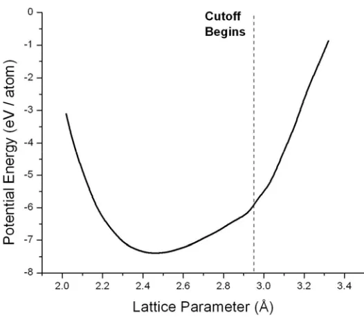
For graphite, application of the REBO potential at 0 K produces the potential energy curve shown in Fig. 2-3.

Fig. 2-3. The potential energy of graphite at 0 K vs. the in-plane lattice parameter, as computed using the REBO potential. At a lattice parameter of 2.94 Å, the 1st neighbor separation enters the cutoff range, causing a sudden increase in the potential energy gradient.

27

Chapter 3

Motivation for a New Model

3.1 Graphite

Structure

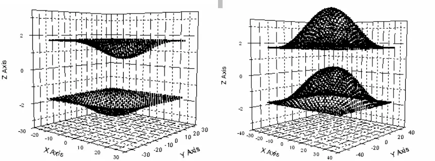
While the REBO potential provides a fairly comprehensive treatment of short-range interactions, no attention is given to the long range forces that are vital to the stability of the graphite structure. The need for an additional component of the potential is illustrated in Fig. 3-1. These snapshots of the simulated atomic positions reveal that an entire plane of atoms may exhibit membrane-like vibrations unless a force is present to resist out-of-plane motion. The unnaturally large vibrations evident in Fig. 3-1 are also manifest in the out-of-plane mean squared displacement, displayed in Fig. 3-2.

Fig. 3-1 The profile of a simulated array of graphite using the REBO potential with fixed boundary atoms. The atomic planes oscillate in an unphysical manner in the absence of long range forces.

28

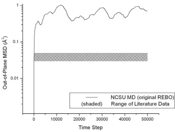
Fig. 3-2. The out-of-plane MSD at 1200 K as computed using the published form of REBO. The calculated MSD approaches equilibrium an order of magnitude above the band of MSD values reported in literature.

However, the explicit inclusion of long range interactions is computationally intensive, since the number of interacting pairs increases many fold. The approach taken in this work is to approximate long-range interactions using a function dependent only upon an atom’s out-of-plane displacement relative to the interplanar spacing of the system (which, in turn, varies with temperature). This function is parameterized so as to fit experimental mean-squared displacement (MSD) data along the hexagonal c-axis.

3.2 Absolute Zero Fitting

29 REBO employs a fitting database consisting only of absolute zero properties such as bond length, force constant, and atomization energy. Consequently, the fitted REBO constants are strictly suitable only at 0 K.

Combined with the general-purpose intent of REBO, this fact suggests that high temperature MD calculations will likely depart from experimental measurements. Indeed, such a discrepancy was found to exist in the thermal expansion coefficient. Fig. 3-3 illustrates the difference between MD and experiment. To improve the performance of REBO at high temperatures, a temperature-dependent adjustment factor is introduced in the present work.

30

Chapter 4

Description of the NCSU MD Model

4.1 Introduction

The final NCSU MD model will now be discussed in detail. A number of non-standard features have been included that specifically address the graphite structure. Unless otherwise noted, all simulations were performed in the NVT ensemble using periodic boundary conditions, at a time step of 0.5 femtoseconds. The flowchart given in Fig. 4-1 illustrates the basic functioning of the NCSU MD code, which is designed to run on parallel processors. Details of the parallelization are discussed in Appendix B.

Fig. 4-1 Flowchart of the NCSU MD code

Initialization

Check time step

Predict x,y,z

Geometry splitting & handshaking

Force Calculation

Correct x,y,z & Apply thermal bath If t < tset

BEGIN

31

4.2 Thermal

Bath

NVT conditions were imposed through a two-step process:

(i) Rescaling of all atomic velocities for several hundred time steps

(ii) Velocity rescaling only within a delimited thermal bath region (along the periphery of the supercell) for the remainder of the simulation

The purpose of step (ii) is to circumvent direct manipulation of atomic trajectories within the interior of the supercell during the “production phase” of the simulation, thereby minimizing perturbation of the system’s time evolution. Following equilibration, quantities of interest were calculated as averages over the interior of the supercell (outside of the thermal bath).

4.3 Interplanar

spacing

32

Fig. 4-2 The C/A ratio for Graphite

4.4 Center of Mass Correction

As mentioned in section 2.7, the standard CM correction scheme functions well for an isotropic system yet performs inadequately for graphite. Because the graphitic basal planes do not interact under the REBO potential, it is possible for each plane to glide at some net velocity while still preserving a total CM velocity of zero for the entire system.

33

4.5 Modifications to the Potential Function

To address deficiencies in the performance of the potential function above 0 K, temperature dependency was introduced into Eq. (2.25), which was re-written as:

(

) ( )

[

( )

]

∑∑

>

+ =

i j i

ij A ij ij R ij

c r z T V r T b V r T

f

E ' _, , , , (4.1)

in which adjustments have been made to the cutoff function and pairwise attractive and repulsive terms. These adjustments are now described in turn.

4.5.1 Anisotropic Cutoff

The cutoff function was augmented with an additional term as follows:

(

r z T

) ( )

f r f

( )

z T

fc ij , c ij c ,

' ,

' _{= +}

(4.2) Here, fc

( )

rij is the standard cutoff function and fc

( )

z,T

' _{is defined as:}

( )

2 2 cos 1 , ' ⎥ ⎥ ⎦ ⎤ ⎢ ⎢ ⎣ ⎡ ⎟⎟ ⎠ ⎞ ⎜⎜ ⎝ ⎛ ∆ − = d z K T z f_c π (4.3)

in which z refers to the c-axis displacement of an atom from its initial position in the basal

plane, ∆d is the interplanar spacing, and K governs the magnitude of the barrier to

out-of-plane motion generated by f_c'

( )

z,T . The appropriate value of K is determined in Chapter 5

by fitting c-axis MSD calculations to experimental measurements. The basic form of fc

( )

z,T

34

Fig. 4-3 Profile of the c-axis cutoff function, f_c'

( )

z,T . The period of f_c'

( )

z,T is equal to the interplanar spacing, which increases monotonically with temperature.

The Lennard-Jones model (often used to simulate Van der Waals forces) also behaves parabolically at small displacements about the equilibrium point. This may be demonstrated analytically from the Lennard-Jones formula [16]:

⎥ ⎥ ⎦ ⎤ ⎢ ⎢ ⎣ ⎡ ⎟ ⎠ ⎞ ⎜ ⎝ ⎛ − ⎟ ⎠ ⎞ ⎜ ⎝ ⎛ = 6 12 2 r r r r V

U e e

e

lr (4.4)

where re and Ve are fitting constants. Expanding Eq. (4.4) with a Taylor series:

(

)

( )

78

(

)

...

12 1 2 2 12 + − + − − ≅ ⎟ ⎠ ⎞ ⎜ ⎝ ⎛ e e e e e r r r r r r r r (4.5)

(

)

( )

42

(

)

...

12 2 2 2 2 6 + − − − + − ≅ ⎟ ⎠ ⎞ ⎜ ⎝ ⎛ − _e e e e e r r r r r r r r (4.6) And therefore:

( )

(

)

⎥⎥_⎦ ⎤ ⎢ ⎢ ⎣ ⎡ − + − ≅ 2 2 36 1 e e e

lr r r

r V

35 at small displacements from re (the minimum energy distance) .

4.5.2 Pairwise Coefficients

The terms V_A

( )

r_ij,T and V_R

( )

r_ij,T in Eq. (4.1) may be expanded as:

( )

( )

[

ij

]

ij ij

R r

r Q T

A T r

V −α

⎥ ⎥ ⎦ ⎤ ⎢ ⎢ ⎣ ⎡

+

= 1 exp

, (4.8)

( )

_∑

( )

[

]

=

− =

3 , 1

exp ,

n

ij n n

ij

A r T B T r

V β (4.9)

where the pairwise potential coefficients,A andB_n, now vary with temperature. The purpose

of this modification is to compensate for the sole usage of 0 K properties in fitting the interatomic potential function, which was shown to be inadequate for graphite even at intermediate temperatures.

Modification of the pairwise coefficients affects the weights of the repulsive and attractive terms, and any change in these coefficients will, in general, affect both the position and depth of the potential energy minimum. Because the thermal expansion coefficient depends upon the position of the potential energy minimum as a function of temperature, correct thermal expansion behavior may be achieved by devising appropriate forms for A

( )

T and Bn

( )

T . The specific methodology used in this work to defineA

( )

T and Bn

( )

T will be

36

Chapter 5

MD Results

5.1 Absolute Zero Properties

The first step in verifying an interatomic potential function is to ensure that it yields correct values for the physical parameters of the system of interest at absolute zero temperature. Two such parameters – the cohesive energy and bond length – are characteristic quantities that are generally well-defined in literature. Fortunately, both are also obtainable from the most basic output of an MD simulation.

The cohesive energy of a crystal is defined as the energy required to dissociate the crystal into a set of infinitely separated atoms at rest [16]. Because the REBO potential does not account for interplanar interaction, determination of the cohesive energy in graphite involves only the in-plane lattice parameters (the a and b parameters). These are related by:

a b

3 2

= (5.1)

so that the cohesive energy is a function only of the a parameter.

37

Lattice Parameter (angstroms)

2.43 2.44 2.45 2.46 2.47 2.48

Energ

y (eV / atom

)

-7.396 -7.395 -7.394 -7.393 -7.392 -7.391

Fig. 5-1 The energy profile as a function of lattice parameter at 0K

Theoretically, the 0 K properties of graphite correspond to the minimum of the energy curve. The deduced equilibrium lattice parameter is therefore 2.46 Å, and the cohesive energy (i.e. the potential energy at the equilibrium lattice parameter) is 7.395 eV/atom. These values exhibit good agreement with experiment as well as previously published results with the REBO potential function [12].

5.2 General High Temperature Behavior

5.2.1 Potential Energy

38

kT E

E E

E _{tot K coh}

2 3 − ≅

−

= (5.2)

where Ecoh is the cohesive energy. While the simulated system is not expected to behave in a purely harmonic manner, Eq. (5.2) should be a rough approximation of the calculated mean potential energy. MD calculations of potential energy are compared to the harmonic approximation in Fig. 5-2.

Fig. 5-2 Mean potential energy vs. temperature. Comparison is made to the harmonic approximation.

Anharmonicity in the potential function is evident through the slight deviation from the harmonic approximation. However, the average MD potential energy exhibits very similar behavior.

5.2.2 Standard Deviation in Temperature

39 temperature control mechanism was then halted abruptly, converting the system to an NVE (constant energy) ensemble. Under the NVE ensemble, the average kinetic energy (and hence also the temperature) fluctuates with an amplitude dependent upon the magnitude of the temperature. To see this, one may start with the statistical uncertainty inherent in one particle’s kinetic energy:

T kB E_K =

σ (5.3) where the total kinetic energy of the system is given by ε = NEK. Therefore,

(

E

)

N

(

kBT

)

kBT N

i

Ki = =

∆

=

∑

2 2

ε

σ (5.4)

and from the classical expression relating kinetic energy to temperature:

T NkB

2 3 =

ε (5.5)

the standard deviation in temperature can be derived as follows:

N T k

Nk_{B T} = _B

= σ

σ_ε 2 3

(5.6)

N T

T

1 3 2 =

σ (5.7)

40 Number of Atoms

1000 2000 3000 4000 5000

Te

mpera

ture

St

anda

rd Dev

iat

ion (K)

0 10 20 30 40 50

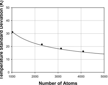
Fig. 5-3 Comparison of the temperature fluctuations of a graphitic system as calculated from MD simulations (dots) and the derived theoretical model (solid curve).

5.3 High Temperature Physical Properties

5.3.1 Thermal Expansion

The linear coefficient of thermal expansion is defined as:

( ) ( )

dT

( )

T da T a

T = 1

α (5.8)

where a(T) is the lattice parameter at temperature T. In a purely harmonic material, the coefficient of thermal expansion is uniformly zero. Thus, expansion (or contraction) arises from higher-order anharmonic terms in the potential energy function.

41 As a consequence of the short-range nature of the REBO potential, the c-axis expansion coefficient could not be examined in this work. However, the a-axis expansion coefficient is an excellent quantity against which to benchmark the NCSU MD code.

Adjustment Factor

It has already been shown that thermal expansion calculations using the published REBO potential do not agree well with experiment. Thus, the discussion now focuses on fitting the functions A

( )

T and B_n

( )

T (as applied in Eqs. (4.8) and (4.9)) to the correct

thermal expansion profile of graphite. For the purposes of this work, A

( )

T and B_n

( )

T were

written as:

( )

T A

[

C

( )

T T

]

A = _oexpα (5.9)

( )

T B

[

C

( )

T T

]

B_n = _n,oexpβ_n (5.10)

where A_o and B_n,o are the constant pairwise coefficients as defined in the published REBO

potential, and C(T) is a temperature-dependent adjustment factor. These forms for A

( )

T and

( )

T

B_n were chosen because they reduce to A_o andB_n,o at T = 0, thereby maintaining

agreement with 0 K properties such as bond length and cohesive energy. The procedure employed to obtain an explicit formula for C(T) shall now be described.

First, an estimation of the sensitivity of the potential energy minimum to C(T) is needed. Due to the small magnitude of the adjustment factor – which is treated as a perturbation to the potential function – the terms exp

[

αC

( )

T T

]

and exp

[

β_nC

( )

T T

]

are

42 of the potential energy minimum is also linear with respect to C(T)T. Therefore, an estimation of C(T) at any temperature may be ascertained via the formula:

( )

( )

[

a T a T

]

a C T

C_{est ref} − _o

∆ = )

( (5.11)

where Cest is the estimated adjustment factor, aref and ao are the reference and calculated

lattice parameters respectively, and ∆a/C is the rate of change in lattice parameter with respect to C (generated from an arbitrary yet reasonable initial guess of C).

It is sufficient to determine the slope, ∆a/C, at one temperature (say 300K) and then utilize this to estimate the value of C(T) required to match experimental data at all other temperatures. Using the procedure outlined above, the normalized slope,

T T C

a

) ( ∆

, was found

to be 0.87.

Applying Eq. (5.11) to the data in Fig. 3-3 results in the estimated C(T) values plotted in Fig. 5-4. The reference lattice parameters were taken as the midpoints of the shaded region of Fig. 3-3.

43

Fig. 5-4 The predicted values of C(T) up to 1800 K.

A sigmoidal fit was chosen because the sigmoid function asymptotically approaches constant values at the low and high temperature extremes, resulting in a constant thermal expansion (or contraction) in these limits, as is observed in graphite. To fit the data of Fig. 5-4, a four-parameter sigmoid function of the following form was used:

(

)

⎥⎦ ⎤ ⎢⎣

⎡− − +

+ =

d T T b c

T C

o o

exp 1 )

( (5.12)

44

Table 5.1: Parameters for Sigmoidal Fit to C(T).

b = 4.769E-06 Å/K d = 3.897E+02 K To = 1.410E+03 K co = -1.681E-06 Å/K

Fig. 5-5 Sigmoidal Fit to the estimated values of C(T)

Substituting the fitted C(T) back into Eqs. (5.9) and (5.10) yields the final formulae for A(T) andB_n

( )

T , which are plotted in Fig. 5-6 Lattice parameter computations were

repeated to confirm that A(T) and Bn

( )

T generate the desired impact on thermal expansion

45

Fig. 5-6. Attractive and repulsive coefficients of the modified REBO potential as a function of temperature, normalized to their (constant) published values. At 0 K the normalized coefficients are identically unity, indicating that there is no impact to the cohesive energy or bond length at this temperature.