WICKER, ANDREW W. Interest-Matching Comparisons using CP-nets. (Under the di-rection of Professor Jon Doyle.)
The formation of internet-based social networks has revived research on traditional
social network models as well as interest-matching, or match-making, systems. In order to
automate or augment the process of interest-matching, we follow the trend of qualitative
decision theory by using qualitative preference information to represent a user’s interests.
In particular, a common form of preference statements for humans is used as the motivating
factor in the formalization of ceteris paribus preference semantics [13]. This type of prefer-ence information led to the development ofconditional preference networks (CP-nets) [6, 5]. This thesis presents a method for the comparison of CP-net preference orderings which
al-lows one to determine a shared interest level between agents. Empirical results suggest that
distance measure for preference orderings represented as CP-nets is an effective method for
determining shared interest levels. Furthermore, it is shown that differences in the CP-net
structure correspond to differences in the shared interest levels which are consistent with
in-tuition. A generalized Kemeny and Snell axiomatic approach for distance measure of strict
partial orderings is used as the foundation on which the interest-matching comparisons are
by
Andrew W. Wicker
A thesis submitted to the Graduate Faculty of North Carolina State University
in partial fulfillment of the requirements for the Degree of
Master of Science
Computer Science
Raleigh, North Carolina 2006
APPROVED BY:
Dr. Peter R. Wurman Dr. Robert St. Amant
Dr. Jon Doyle
BIOGRAPHY
Andrew White Wicker was born on December 11, 1981 and raised in Greensboro, North
Carolina, just one hour west of North Carolina State University. Upon receiving a Bachelor
of Science degree in Computer Science with a minor in Mathematics at North Carolina
State University, he decided to continue in the graduate program to pursue his interest in
ACKNOWLEDGEMENTS
I would like to thank Dr. Jon Doyle for his time and support throughout the research for
this thesis. His attention to detail and highest expectations for research quality pushed me
to achieve a level of intellectual development unforeseeable at the beginning of my graduate
Contents
List of Figures vii
1 Introduction 1
1.1 Outline of Problem . . . 1
1.2 Approach . . . 2
1.3 Contributions . . . 3
1.4 Organization of Thesis . . . 4
2 Preferences 5 2.1 Types of Relations . . . 5
2.2 Preference Notation . . . 6
2.3 Ceteris Paribus Semantics . . . 7
3 Conditional Preference Networks 9 3.1 ConditionalCeteris Paribus Preference Statements . . . 9
3.2 CP-net Structure . . . 10
3.3 CP-net Semantics . . . 13
3.4 Reasoning with CP-nets . . . 15
4 Measuring Similarity 17 4.1 An Axiomatic Approach . . . 17
4.2 Representation for Comparisons . . . 19
4.3 A Simple Comparison Example . . . 21
5 CP-nets in a Multi-agent Environment 22 5.1 Agent Preferences as CP-nets . . . 22
5.2 Definition of Terms . . . 23
5.3 Restrictions and Structural Assumptions . . . 24
5.4 Feature-based Case Analysis . . . 25
6 Comparing Preference Orderings Represented as CP-nets 26 6.1 Preference Graph Based Ordering Matrix Construction . . . 26
6.3 Shared Interest Function . . . 29
6.4 Computing Shared Interest using CP-nets . . . 31
6.5 CP-net Shared Interest Algorithm . . . 33
7 CP-net Variations 36 7.1 Defining CP-net Permutations . . . 36
7.2 Relation between Shared Interest Values . . . 38
7.3 Feature Subset . . . 41
7.4 Variations in both Feature Sets . . . 44
7.5 Topological Differences . . . 46
7.6 A Structural Approach to Distance Measure . . . 51
8 Related Work 53 8.1 Ontology-based Approach . . . 53
8.2 mCP-nets . . . 54
9 Concluding Remarks 55 9.1 Future Work and Open Problems . . . 56
Bibliography 58 A Notation Definitions 62 B Application Source Code 64 B.1 Overview . . . 64
B.2 CPNet class . . . 64
B.3 Feature class . . . 71
B.4 FeatureAtom class . . . 74
B.5 Outcome class . . . 75
List of Figures
3.1 A simple CP-net using just two feature nodes . . . 11
3.2 A simple CP-net using three feature nodes . . . 13
3.3 Induced preference graph . . . 14
6.1 Two CP-netsN1 and N2 . . . 32
7.1 Example flipping function . . . 37
7.2 An atomic flipping of one row of CPT(B) . . . 37
7.3 CPT-flipping functionπB . . . 38
7.4 Two CP-netsN3 and N4 . . . 39
7.5 CP-netN5 . . . 41
7.6 Induced preference graphP(N5) . . . 42
7.7 Expanded (disconnected) preference graph fromP(N5) . . . 43
7.8 CP-netN6 . . . 44
7.9 Induced preference graph forN6 . . . 45
7.10 Another expanded (disconnected) preference graph fromP(N5) . . . 45
7.11 Expanded (disconnected) preference graph forN6 . . . 46
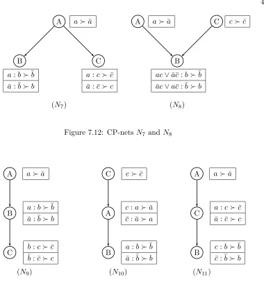
7.12 CP-nets N7 and N8 . . . 47
Chapter 1
Introduction
It is natural for humans to apply new technology to a social context if it is useful
in any way. With the advent of the personal computer, and subsequently the internet,
users of these tools have discovered both mundane and ingenious ways for facilitating social
interaction with other users. It was not long before people began constructing ad-hoc social
networks through, for example, mailing lists and forums. These early “social networks”
eventually evolved into the more interactive and media-rich social networks that can be
seen today (e.g., MySpace.com and FaceBook.com).
Internet-based social networks have become a place where people can go to see
and be seen by others. Nearly all of the popular social network sites allow users to upload
detailed information about themselves along with photos and other types of multi-media.
This helps to create the interactive experience which causes people to continually update
their profile, as well as add new friends to their personal social network. This is done
typically by querying the database of users for other users that share a common interest.
The social network interaction, expansion, and profile updates are what keep users engaged.
1.1
Outline of Problem
An increasing amount of work has been done on formalizing what it means for two
as interest-making, or match-making. A decision to interact with another person is based
strongly on what level of interest is associated with some aspect of that person. These
aspects often are a similarity of preference or desires. Although basic notions of
interest-matching are not novel ideas, there are numerous approaches to this problem which offer
their own advantages and disadvantages [9].
In order to automate or augment the process of interest-matching, it is helpful
to develop a model which formalizes the characteristics of a person that are necessary for
making this sort of decision. Preference information is a natural way of capturing what
it is that a person wants or intends to do. In particular, conditional preference networks
(CP-nets) are a natural, compact representation of preference information operating under
the ceteris paribus semantics [6, 5, 13].
This thesis describes a reasonable method for facilitating interest-matching
com-parisons between users in a social environment that uses preference information represented
as a CP-net. Furthermore, distance measures of orderings are shown to be capable of
com-puting reasonable and intuitive interest levels.
1.2
Approach
These on-line social networks are especially intriguing when viewed in the context
of multi-agent systems. Each user in the network can be thought of as an individual agent
with specific preferences, desires, intentions, and/or goals. The interpretation of a social
network environment as a multi-agent environment more easily facilitates formalization of
the social interactions using decision-theoretic models.
The social networks now in place have methods through which users are able
to expand their network which is based on a level of interest in another user’s profile
information. A CP-net provides a formal model for representing a user’s preferences, which
are necessary for making a network expansion decision. It is shown how comparisons can be
made between CP-nets of multiple users in an attempt to measure a level of shared interest.
There has been much research conducted on distance measures between orderings
over objects [2, 3, 15]. This thesis makes use of a generalized Kemeny-Snell axiomatic
approach described by Bogart [2] to form comparisons between CP-net preference orderings.
when using the preferences represented in CP-nets.
1.3
Contributions
This thesis describes a step toward a potential application of CP-nets in a
so-cial multi-agent environment. Research on CP-nets has not fully explored this application
area. Closely related work on mCP-nets focuses on aggregating preference information of multiple agents for group consensus [20], which is in contrast to the individualistic view
of agent decision-making that has motivated work on this thesis. By allowing the agents
to make decisions based on individual interest-matching comparisons (as opposed to group
consensus), they are afforded more freedom in their decision-making process.
A generalized Kemeny-Snell axiomatic approach to measuring distance between
strict partial orderings is described [2]. We build on this approach by defining a method
for modifications of CP-nets, called CP-permutations, which consequently result in modifi-cations to the preference orderings they represent. It is discussed how these modifimodifi-cations
could be used to define a much more efficient axiomatic approach to measuring distance
between the actual CP-net structure, not the induced preference orderings.
Several problems that are common for interest-matching systems are outlined in
[9]. The approach to interest-matching described in this thesis addresses a couple of these
problems. First, many interest-matching systems do not allow ranking of interest levels
between multiple agents. By using the interest function that is described in this thesis,
rankings of interest values are permitted since the values are normalized (i.e., they are
in-dependent of the size of the preference orderings being compared). Second, exact matches
of outcome domains over which the preferences are specified are often required in
interest-matching systems. We describe an induced preference graph expansion method which allows
one to make comparisons even if the feature sets (hence, outcome sets) over which the
pref-erence orderings are defined are significantly different. This allows one to make partial, or
potential interest matches.
An overarching motivation for this thesis is the foundation it lays for extending
CP-nets to a social multi-agent environment by defining a formal method for determining
shared interest levels between them. This method could be utilized in a multitude of
possess similar preferences, desires, or goals. A framework for this sort of application is the
next logical step for future work on this thesis topic.
1.4
Organization of Thesis
This thesis begins with a discussion of a preferences, in which we describe basic
types of relations, preference notation, and theceteris paribussemantics. Theceteris paribus
semantics is built-upon in Chapter 3 with the introduction of CP-nets. The structure of
CP-nets is discussed, along with techniques for reasoning with them. In Chapter 4, we
lay out the generalized Kemeny-Snell axiomatic foundation on which the interest-matching
comparisons are based. Chapter 5 describes some of the relational and structural properties
of CP-nets in a multi-agent environment. Chapter 6 introduces the shared interest function
used to make comparisons between CP-nets, and discusses how the generalized
Kemeny-Snell axioms apply in the context of preference orderings represented as CP-nets. Several
examples are provided in Chapter 7 which show how the interest-matching comparisons are
computed when variations between CP-nets are introduced. This thesis concludes with a
Chapter 2
Preferences
If one wants to define a method through which interest-matching comparisons are
made, then it makes sense to use preferences as the comparative information. Preferences are
a natural way to express desires, plans, and goals [23]. Furthermore, qualitative preference
information is especially easy for humans to state, and less prone to error, in comparison
to quantitative utility information [11].
Preference information that has been elicited from a user can be stated over many
types of relations. It is important to recognize the differences between these relations. In
this chapter, we look at types of relations used to define various types of orderings. This
discussion continues with a description of the ceteris paribus preference semantics.
2.1
Types of Relations
Prior to continuing with a more in-depth look at preference semantics and
repre-sentation, it is helpful first to take a look at basic relations of preference statements. We
emphasize an ordering over the set of outcomes which represents the desirability of an
out-come.
pairs R ⊆O2. The set notation (o, o′) ∈ R is used instead of the relational notation oRo′
to denote a relation between o ando′ [19, 18].
Definition A relation R on O is reflexive if and only if (o, o) ∈ R for each o ∈ O. A relation R onO isirreflexive if and only if (o, o)6∈R for each o∈O.
Definition A relationR onO issymmetric if and only if (o, o′)∈R implies (o′, o)∈R for each o, o′ ∈O. A relation Ron O isantisymmetric if and only if (o, o′)∈R and (o′, o)∈R
imply o=o′ for each o, o′ ∈O. A relation R on O is asymmetric if and only if (o, o′)∈R
implies (o′, o)6∈R for each o, o′ ∈O.
Definition A relationR onOistransitive if and only if (o, o′)∈R and (o′, o′′)∈Rimplies (o, o′′)∈R for each o, o′, o′′∈O.
Definition A preorder is a reflexive and transitive relation.
Definition A partial order is an antisymmetric preorder.
Definition A strict partial order is an irreflexive, transitive, and asymmetric relation.
Definition An ordering iscomplete if and only if (o, o′)∈Ror (o′, o)∈Rfor eacho, o′ ∈O.
Definition A weak order is a complete and transitive relation.
There are many other types of orderings defined over these relations that are not mentioned
in this thesis. We are concerned primarily with the weak ordering and strict partial ordering.
If an ordering type is not specified, or irrelevant in the context of the specific problem, then
we will refer to it as simply an ordering.
2.2
Preference Notation
Three distinct degrees of preferential ordering are used in the general description
of an agent’s preferences. Let o and o′ be outcomes from a set of outcomes O of executing an action (or, more generally, propositions) on which an agent can place a relation. It is
assumed that a complete preorder is placed over Oby the relation%[23]. When oisweakly preferred to o′, we write o%o′. We define o≻o′ asstrict preference of o over o′ ifo%o′
and o′ 6%o. Ifo%o′ and o′ %o, we write o∼o′ and define this as indifference between o
2.3
Ceteris Paribus
Semantics
Some human preferences are commonly a type of multi-attribute preference that
can be stated formally by preference statements operating under the ceteris paribus se-mantics [13]. This type of preference sese-mantics takes an “all else equal” approach when
considering alternatives in a decision-making context. Traditionally, decision-theoretic
ap-proaches taking advantage of preferences attempt to define an ordering over all outcomes.
The problem with this is that most planning systems suffer from a combinatorial explosion
with the set of possible outcomes. Enumerating all of these is incredibly inefficient, and
sometimes impossible. To avoid this inefficiency, the ceteris paribus semantics is used to lift preference statements to preferential patterns that exist over classes of outcomes (or
possible worlds).
Ceteris paribus preference semantics assumes outcomes are described by a set of binary features F. The features in the set F are capable of describing all of the possible classes of outcomes derivable from our decision-making process. We define preferences for
outcomes described in terms of features inF over others throughceteris paribus preference statements.
Leto=habci and o′=h¯abcibe outcomes, whereF ={A, B, C}. Assume that we have the following ceteris paribus preference rule: a≻¯a. This rule states a preference fora
over ¯a, assuming that all other features inF are held constant. The preference statement is operating under the ceteris paribus semantics if it holds true when the truth values for all features other thanaand ¯aare the same and held constant. Another way of saying this is, every class of outcomes satisfying ais preferred to those satisfying ¯aif all other features in these statements are the same and held constant. Given the two outcomes oand o′, we would state a preference for o over o′, written o≻ o′, based on this single ceteris paribus
rule since the features B and C not mentioned in the rule are the same and held constant in both o ando′.
As a less formal example, consider the case of placing preference on airplane flights.
There are typically many features to consider when choosing the best, most preferred flight.
We specify that cheaper flights are preferred to shorter flights, all else equal. So, we prefer
flights that are cheap and not short to flights that are not cheap and short, if all other
features relevant to an airplane flight are the same in the alternative outcomes being
We turn our attention now to a graphical representation for preference using a
Chapter 3
Conditional Preference Networks
Often it is desirable in automated decision support systems to make decisions using
a qualitative specification for preferences, as opposed to a quantitative specification. Of
specific interest are conditional preference networks (CP-nets), which specify a qualitative and conditional factored representation of preferences in a graphical network [6, 5, 10].
By using conditional ceteris paribus preference statements a CP-net exploits independence relations between these preference statements to produce a compact, intuitive, and
well-structured graphical model.
3.1
Conditional
Ceteris Paribus
Preference Statements
As stated, CP-nets represent conditional preferences operating under the ceteris paribus semantics. An example of a conditional preference is provided: “If I drink coffee, I prefer that it has sugar in it.” That is, my preference for sugar is dependent on the condition that I am drinking coffee. Applying the semantics of ceteris paribus statements, we conclude that the statement about coffee holds true “all else equal”. It does not depend
on the temperature or type of coffee if it is the same for all coffee under consideration.
The general form of the notation used for these conditional statements isa: b≻¯b
This notation provides a compact qualitative specification for potentially complex preference
statements.
3.2
CP-net Structure
When constructing a CP-net, it is necessary first to elicit preference information
from the user. This is done by having the user specify influence relations between preference
features. The influence relations represent a preference feature independence assumption
that is critical to CP-nets and permitted by the use of the conditionalceteris paribus prefer-ence semantics. This assumption is analogous to the probabilistic independprefer-ence assumption
used in Bayesian networks, however, it is a weaker notion of relations between nodes.
We describe a standard format of the outcomes being used throughout the
re-mainder of this paper. This is done by defining an enumerated finite universe of features
denoted by F = hf1. . . fni. The finite universe of features F contains the features from
which we are able to construct all CP-nets used in this thesis. The ordering of the features
in the enumeration carries with it no semantical meaning and is used only to permit direct
comparison of ordering matrices (see Chapter 6).
Each featuref in a CP-net can be instantiated over a domain of values, Dom(f). For specifying a standard format for outcomes, let OF =Q
f∈FDom(f) be the set of out-comes over F. Each outcome inOF is a n-tuple, where f ∈F and |F|=n. We denote the outcomes over F ⊂ F by OF. Given OF, we say OF′ is a set of partial outcomes, where
F′ ⊂F. A partial outcome is sometimes referred to as an instantiation. It is worth pointing out that the formal specification of a CP-net allows for arbitrary finite domains, but we
assume |Dom(f)|= 2 for eachf ∈Fthroughout this paper [6, 5].
As a simple example, letF={A, B, C}. Thus, the set of all outcomes isDom(A)×
Dom(B)×Dom(C). For a CP-net N, where F = {A, C} ⊂ F, the outcomes will be for-matted as Dom(A)×Dom(C).
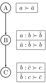
A
B
a≻a¯
a:b≻¯b
¯
a: ¯b≻b
Figure 3.1: A simple CP-net using just two feature nodes
and Y arepreferentially independent if and only if it is true for all x1, x2, y1, y2 that
x1y1%x2y1 ⇐⇒x1y2%x2y2 (3.1)
We say that x1 is preferred to x2 if the above relation is true [6, 5]. The notion of conditional preferential independence is defined by introducing a third set of featuresZ
such that the nonempty sets X,Y, and Z partition the set F. Given z∈OZ, we say X is conditionally preferentially independent ofY if and only if it is true for allx1, x2 ∈OX and
for all y1, y2∈OY that
x1y1z%x2y1z⇐⇒x1y2z%x2y2z (3.2)
The relation stated above is interpreted as saying thatX and Y areconditionally preferen-tially independent in the case when Z is instantiated asz.
The structure of a CP-net, as considered in this thesis, is defined formally in
graph-theoretic terms as a directed acyclic graph (DAG). There has been much work on cyclic CP-nets, but they are not considered in this thesis [5]. Each node in a CP-net
N = (F, E) is labeled by a single feature f ∈ F. The parents of a feature node f in a CP-net N are denoted asP a(f). A feature node fj is a parent of fi, that isfj ∈ P a(fi), if there exists a directed edge in the CP-net from fj to fi. The acyclicity of the CP-nets considered in this paper maintains that inconsistencies will not appear in the feature node
relations.
A set of feature influence relations forms a dependency relation on all features.
example using just two features, Aand B [6, 5]. The user specifies that B isconditionally preferentially dependent onA. Furthermore, the user specifies a preference foraover ¯a(i.e.,
a≻¯a),b over ¯b givena (i.e.,a:b≻¯b), and ¯b over bgiven ¯a(i.e., ¯a: ¯b≻b). The structure of the basic CP-net that is constructed from this dependency information is depicted in
Figure 3.1.
Note that each node in Figure 3.1 is annotated with a conditional preference table
(CPT). This is similar to the conditional probability tables of Bayesian networks. These CPTs provide a compact description of a user’s complete preference ordering for domain
values of a feature node f over every instantiation of its parent feature nodes, denoted by
OP a(f). So, for feature nodeB we have botha:b≻¯band ¯a: ¯b≻b in its CPT.
We call instantiation u ∈ OP a(f) a partial outcome since P a(f) ⊂ F. Each u ∈
OP a(f) provides a complete order≻u
f over Dom(f) [5]. For example, letF ={A, B, C}and
let u=a¯b∈OP a(C), whereDom(A) ={a,¯a}andDom(B) ={b,¯b}. Then, from Figure 3.2 we have c≻u
C ¯c.
Let NF be the set of all CP-nets definable over feature set F ⊆F and let N =
S
F⊆FNF be the set of all CP-nets.
Definition A CP-net N ∈ NF is a directed graph over feature nodesF, each nodef ∈F
of which is annotated with a conditional preference tableCP T(f). EachCP T(f) associates a complete order ≻u
f with each u∈OP a(f).[5]
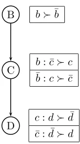
An example with more detailed preference information is provided. Assume a user
has specified a preference for aover ¯a(i.e.,a≻¯a), bover ¯bgiven a(i.e.,a:b≻¯b), ¯b overb
given ¯a(i.e., ¯a: ¯b≻b), ¯c over cgiven b(i.e., b: ¯c≻c), and cover ¯c given ¯b (i.e., ¯b:c≻¯c). A root node in a CP-net is specified as an unconditioned preference. The feature
A will represent the root node in our CP-net for these dependencies since its preference is unconditioned, and thus has no parents. The featuresB andCwill be internal nodes where
A is the parent ofB, andB is the parent of C. The graphical structure for the CP-net that is constructed from these dependency relations is depicted in Figure 3.2. The nodes in this CP-net represent the features of interest to the user. Clearly, there is exactly one node for
A
B
C
a≻a¯
a:b≻¯b
¯
a: ¯b≻b
b: ¯c≻c
¯b:c≻c¯
Figure 3.2: A simple CP-net using three feature nodes
3.3
CP-net Semantics
Now that a graphical representation of preference information has been constructed
we are able to define the semantics of the CP-net to determine a preference ordering derived
from the CPTs. The relations in the CPTs define a strict partial ordering over outcomes
OF.
Let ΩF be the set of all strict partial preference orderingsω over outcome setOF
and let Ω =S
F⊆FΩF be the set of all strict partial preference orderings.
We say that a preference ordering ω satisfies a CP-net if and only if it satisfies the conditional preferences in each of the CPTs. A preference ordering ω that satisfies a CP-net N is interpreted as the meaning of that CP-net, denoted by ω = [[N]]. So, if a CP-net N ∈ NF, then [[N]]∈ΩF.
In the remainder of this paper, we will denote the inclusion of a preference for o
over o′in the orderingωby either (o, o′)∈ωor by the subscript notation as ino≻ω o′. The
later will be used when dealing with large preference orderings since set notation quickly
becomes unmanageable. The standard notation for the strict preference relation≻, without
a subscript, is used whenever the source of the preference order is clear from the context.
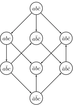
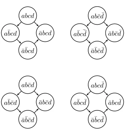
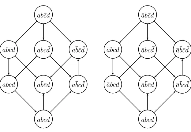
The following preferential ordering satisfies the CP-net in Figure 3.2:
ab¯c
abc
a¯bc
a¯b¯c
¯
a¯bc
¯
a¯b¯c
¯
ab¯c
¯
abc
Figure 3.3: Induced preference graph
There are two types of flipping sequence: worsening and improving. A worsening flip is defined as the change in a single value of an outcome such that the newly created outcome
is less preferred than the original. Conversely, an improving flip is defined if the newly created outcome is more preferred than the original. A sequence of one of these types of
flips is called a flipping sequence. This idea forms the mechanism through which reasoning takes place in CP-nets.
Based on the CPTs in Figure 3.2, one might be tempted to state the preference
a¯bc¯≻¯a¯bc. However, this preference violates the flipping sequence semantics since a¯bc¯and ¯
a¯bc differ by more than a single feature value and there does not exist a flipping sequence containing a¯b¯c ≻ a¯¯bc. Thus, this preference statement does not hold with respect to the CP-net 3.2 and is not included in the preference ordering (3.3) [6]. The specification of the preference ordering is perhaps best described through the preference graph induced by the
CP-net it represents.
where N ∈ NF. If we do this with the induced preference graph in Figure 3.3, we get the
following two preference paths:
ab¯c≻abc≻a¯bc≻a¯b¯c≻¯a¯bc¯≻¯ab¯c≻¯abc (3.4)
ab¯c≻abc≻a¯bc≻¯a¯bc≻¯a¯bc¯≻¯ab¯c≻¯abc (3.5) These two preference paths are identical in their preference for all outcomes,
ex-cluding a¯b¯cand ¯a¯bc. Since a preference relation cannot be stated between a¯bc¯and ¯a¯bc, we say that CP-net 3.2 leaves them incomparable.
3.4
Reasoning with CP-nets
Let o=hx1x2. . . xni and o′ =hy1y2. . . yni be two outcomes, wherexi and yi are
feature instantiations. Our goal is to determine whether o′ ≻ o by using the preference information represented in the CP-net. We determine the validity of this preference, and
thus define the semantics for CP-nets through finding a worsening or improving flipping
sequence [6, 5]. These two differ only in the direction in which the search proceeds, although
construction for one might be much more simplified. A worsening flipping search finds a
flipping sequence from the more preferred outcome to the less preferred outcome through a
sequence of less preferred outcomes. The converse is true for defining an improving flipping
search.
We say that a CP-net N entails a preference o≻ o′, written N |=o ≻ o′, if and only if o ≻ o′ is not violated in any preference ordering that satisfies N. In other words,
N |= o ≻ o′ if and only if (o, o′) ∈ [[N]]. The following lemma states that entailment, denoted by |=, of preferences represented in a CP-net is transitive. This transitivity is
easily determined through paths in the induced preference graph. The usefulness of this
lemma is stated in Section 6.1 when we describe an ordering matrix construction method using CP-net preference orderings.
Lemma 3.4.1. For a CP-net N ∈ NF and outcomes o, o′, o′′ ∈ OF, if N |= o ≻ o′ and N |=o′ ≻o′′ then N |=o≻o′′.[5]
Both the worsening search and improving search can be viewed as a graphical
worsening search, we define the root node as o′ = hy1y2. . . yni. The children of any node
in this graph represent those which are less preferred by flipping exactly one feature value
f to f′, in accordance with the CPTs, such that f ≻ f′. Once the entire graph has been properly constructed in accordance with the CPTs, we can determine whether N |=o′ ≻o
by finding a path in the worsening search graph from root node o′ to a node o. This test is polynomial in the number of feature nodes for the acyclic (poly)tree-structured CP-nets
Chapter 4
Measuring Similarity
In order to compute interest-matching comparisons between CP-net preference
orderings, an interest function and a representation of a CP-net preference ordering are
defined. Each of these must preserve the semantics of the original CP-nets. Graph-theoretic
isomorphism can tell us that two CP-nets are structurally identical, but does not take into
consideration semantic differences captured in the CPTs. In this chapter, we take a look at
an axiomatic approach for defining distance functions for strict partial orderings.
4.1
An Axiomatic Approach
There has been a tremendous amount of work on comparing basic orderings, or
rankings, of qualitative data. A well-known example of this work is that of Kemeny and
Snell [15, 17]. Kemeny and Snell lay out a satisfiable set of distance function axioms for
comparing weak orderings. There are several advantages to using this approach. First, the
axioms define a solid foundation on which to base comparisons. Second, a representation
for orderings is provided which conforms to the axioms. Finally, the axiomatic foundation is
instrumental in forming theoretical properties within the context of interest-matching
com-parisons considered in this paper. Because of these benefits, we investigate the Kemeny-Snell
axioms as a basis for our comparison measures.
the Kemeny-Snell axioms of weak orderings to be consistent under strict partial orderings
(i.e., transitive, asymmetric, and irreflexive relations). The work of Bogart in [2] specifies
slight modifications to the Kemeny-Snell axiomatic approach such that these modified
ax-ioms generalize the distance function to be consistent over strict partial orderings. These
generalized axioms are discussed, and we will refer to these as the generalized Kemeny-Snell
axioms.
There are a total of seven generalized Kemeny-Snell axioms that Bogart states
are necessary for determining a distance function for comparing strict partial orderings.
Let ω, ω′, ω′′ ∈ ΩF be three strict partial orderings. Let dΩ : Ω×Ω → ℜ be a distance function on strict partial orderings. We say that ordering ω′ is between ω and ω′′, written as B(ω, ω′, ω′′), if:
1. (i, j)∈ω′ if (i, j)∈ω and (i, j)∈ω′′
2. (i, j)∈ω or (i, j)∈ω′′ if (i, j)∈ω′
Using the set-theoretic notation, we can state these conditions for B(ω, ω′, ω′′) succinctly by ω∩ω′′⊆ω′ ⊆ω∪ω′′ [2].
We state the generalized Kemeny-Snell axioms below with the axiom name used
by Bogart in parentheses [2]. Axioms 1−3 state the basic properties that all distance
functions should satisfy.
Axiom 1 (D1). dΩ(ω, ω′)≥0, and equality holds iff ω =ω′.
Axiom 2 (D2). dΩ(ω, ω′) =dΩ(ω′, ω).
Axiom 3 (D3). dΩ(ω, ω′) +dΩ(ω′, ω′′)≥dΩ(ω, ω′′), and equality holds iff B(ω, ω′, ω′′).
The next axiom is referred to as the “change of mind” axiom. Basically, two
agents that have completely opposite preference orderings should have a maximum
dis-tance between them. The complete opposite preference ordering of ω is denoted byω−1 =
{(i, j)|(j, i) ∈ ω}. Let ∅ denote the empty strict partial ordering (i.e., the strict partial
ordering that makes no comparisons):
Letω′′ be a preference ordering disjoint from the preference orderingsω andω′. If
ω andω′ differ by the sameω′′, then the distances should be equal. This leads to axiom 5:
Axiom 5 (T5). If ω′′ is a preference ordering disjoint from ω and ω′ (i.e., ω∩ω′′=∅=
ω′∩ω′′), then dΩ(ω, ω∪ω′′) =dΩ(ω′, ω′∪ω′′).
The next axiom states that distance function is invariant with respect to
permu-tations, or relabeling, of the set of outcomes in each ordering. A permutation function
π :OF → OF, as it is used here, is defined as a bijective mapping from a set of outcomes
back onto itself. For any preference ordering ω, defineπ[ω] ={(π(i), π(j))|(i, j) ∈ω}.
Axiom 6 (P6). Ifπ :OF →OF is a permutation function, thendΩ(ω, ω′) =dΩ(π[ω], π[ω′]).
The seventh and final axiom is simply for specifying a unit of measure.
Axiom 7 (D7). The minimum positive distance is 1.
Bogart shows that axioms 1− 7 are satisfiable by a distance function on the
collection of strict partial orderings of a set of outcomes, or on some subset of this collection.
4.2
Representation for Comparisons
It is necessary to specify a representation for the orderings we intend to compare
that conforms to the generalized Kemeny-Snell axioms in the context of strict partial
or-derings. First, we define a matrix representation for preference orderings [15, 17, 2, 3]. We
call the matrixM = [mij] anordering matrix [15]. The notation for ordering matrix entries mij is interpreted as mcolumn,row. For an ordering ω, we construct a matrix M = [mij],
where
mij =
1 ifiis strictly preferred toj,
−1 if j is strictly preferred toi,
0 otherwise.
(4.1)
1. mii= 0 (Irreflexivity)
2. mij =−mji (Symmetry)
3. If mij ≥ 0 and mjk ≥ 0, then mik ≥ 0; mik = 0 only if mij = 0 and mjk = 0.
(Transitivity)
Kemeny and Snell state that anordering matrix is in canonical form if the labeling of the matrix columns and rows is consistent with the preference ordering. As an example,
let red ≻green ≻ blue be an ordering such that red is preferred to green is preferred to
blue. Using the definition of theordering matrix for an ordering, we have
r g b
M =
0 −1 −1
1 0 −1
1 1 0
where the columns, and rows, are labeled as hred, green, bluei [15].
Having stated the seven generalized Kemeny-Snell axioms and a satisfying
repre-sentation for an ordering, we must now define formally the distance function. The
exis-tence of this distance function is stated in the following Bogart theorem of the generalized
Kemeny-Snell axioms [2]:
Generalized Kemeny-Snell Theorem 1 (existence theorem). There is at most one distance function on the collection of all strict partial orderings over a set of outcomes satisfying axioms 1−7.
The existence proof of the generalized Kemeny-Snell distance function is a case-based
in-duction proof over the number of outcomes and the reader is referred to [2] for the proof.
Let M = [mij] and M′ = [m′ij] be two ordering matrices representing the preference order-ings ω andω′, respectively. The following Bogart theorem of the generalized Kemeny-Snell axioms defines the unique distance function dΩ:
Generalized Kemeny-Snell Theorem 2 (uniqueness theorem). The function
dΩ(ω, ω′) = 1 2
n
X
i=1
n
X
j=1
represents the unique distance function satisfying the generalized Kemeny-Snell axioms1−7
on the collection of all strict partial orderings over a set of outcomes.
The uniqueness proof is omitted in this thesis and, once again, the reader is referred to [2]
for the proof.
4.3
A Simple Comparison Example
We will walk through an example of a comparison using the generalized
Kemeny-Snell distance function on two orderings. Let red≻ω green≻ω blue and blue ≻ω′ red≻ω′
greenbe two complete orderings over the same set of objects{red, green, blue}. From these orderings, we construct the followingordering matrices using the generalized Kemeny-Snell representation. We rearrange the columns and rows of matrix M′ so that the columns and rows match the labeling hred, green, bluei, as in matrix M. So, we have
M =
0 −1 −1
1 0 −1
1 1 0
M′ =
0 −1 1
1 0 1
−1 −1 0
The reason for rearranging the matrix is that we want to be able to make
compar-isons between corresponding column vectors. If we iterate over the ith column vectors in each matrix, then we know that they correspond to the same object. This rearrangement
provides a standard representation form between the two orderings, which more easily
fa-cilitates comparisons (see Section 6.2).
Using the distance functiondΩ, we find that
dΩ(ω, ω′) = 1 2 3 X i=1 3 X j=1
|mij−m′ij|=
1
2(2 + 2 + 4) = 4 (4.3)
In the next chapter, we consider basic properties of CP-nets when applied in a
social multi-agent environment. Assumptions and restrictions are stated, as well as relations
Chapter 5
CP-nets in a Multi-agent
Environment
There has been increasing interest in CP-nets which has led to variations such as
UCP-nets [4], which incorporate numerical utility into the CPTs, and TCP-nets [7], which
take into account trade-offs by defining relative importance relations. This research on
CP-nets, however, has explored minimally the basic properties of CP-nets in multi-agent
environments [20]. In this chapter, we look at what assumptions should be made and what
properties exist at a structural level between CP-nets in a social multi-agent environment.
5.1
Agent Preferences as CP-nets
The motivating factor for the interest-matching comparisons between preferences
in CP-nets described in this thesis is the application of CP-nets to social multi-agent
envi-ronments. Two critical elements of a multi-agent environment are described briefly using
CP-nets: agent representation and methods for agent interaction [21].
We consider a multi-agent environment in which each agent has associated with it
preferences represented as a CP-net. A multi-agent system often requires some formalism
CP-net allows us to take advantage of the formal semantics of the CP-net (assumingceteris paribus semantics). Also, the number of outcomes over whichceteris paribus preferences are stated is exponential in the number of features. Thus, the compact CP-net representation
is a practical option, in terms of space requirements, for representing these human-type
preferences within a multi-agent environment.
Decision-theoretic frameworks are applied heavily in multi-agent systems [21].
These have traditionally used purely quantitative information about the agent’s preferences
and intentions. The introduction of qualitative decision theory (as opposed to traditional
decision theory) has caused a marked increase in attempts to define typical agent behavior
in qualitative terms [11, 23]. Using a CP-net to represent the preferences of an agent follows
this trend.
Building on the influence of qualitative decision theory, we provide a method for
computing interest-matching comparisons between the CP-nets of different agents. This
method could be used when constructing a decision-theoretic framework in which the agents
interact with each other in some manner. The mechanisms through which the agents
col-laborate, or coordinate, could take advantage of the comparison described in this paper to
determine whether another agent has matching interests. The actions of one agent with a
matching preference to another agent could be instrumental in helping achieve some goal,
or task. The Markov model of a “reasonable man” is one such early attempt by Bogart
at describing a decision-making process along these lines based on a weak theory of
prefer-ence behavior [2]. The remainder of this chapter details some of the properties that these
CP-nets should exhibit in a multi-agent environment.
5.2
Definition of Terms
We use subscript notation to define a CP-net for agentiasNi ∈ NF with outcomes OF. The CPTs inNi are denoted byCP Ti(f) for each f ∈F. We also denote the feature
set for Ni by Fi. We define P(Ni) as the preference graph induced byNi. The preference
5.3
Restrictions and Structural Assumptions
The definition of a CP-net (see Section 3.2) allows for much more generality than is necessary for the types of comparisons considered in this thesis. For example, cycles are
not prohibited in the general definition of a CP-net. However, the presence of cycles
intro-duces problems with respect to transitivity and, hence, consistency. Another issue with the
general definition is the potentially large domain over which features take on their specific
values. There is absolutely nothing that requires the domain to be restricted to a certain
number of possible values [6, 5].
We place the following restrictions on those CP-nets used throughout the
remain-der of this thesis:
1. All feature value assignments are over a binary domain (i.e., for eachf ∈F,|Dom(f)|= 2)
2. All CP-nets are structured as a directed acyclic graph (DAG)
Features are restricted to having binary domains due to the simplicity of
compar-ison measures in the context of interest matching. By restricting the domain of all features
to a binary domain, we remove potential complications that can arise when generalizing a
comparison measure to a mixed-domain environment. For example, a CP-net (in general)
could have one feature with a binary domain and another with a ternary domain.
Most work on CP-nets has focused on acyclic structure, but some work has been
carried-out on CP-nets with cycles [5]. There are some interesting theoretical properties to
be noted in cyclic CP-nets, but these are generally restricted to certain problems that are
not of interest to the area of application in this paper. Thus, the second restriction states
that we ignore the issues with cyclic CP-nets by considering only those CP-nets structured
as DAGs. By doing this, we ensure that all agents whose CP-net preferences are being
compared will behave in a rational manner. Another benefit to this restriction has to do
with the known and/or more efficient complexity results for specific types of these structures
5.4
Feature-based Case Analysis
The feature sets of two CP-nets divide into four cases. Let Ni, Nj ∈ N be our
example CP-nets. The feature setsFiandFj can be used as the differentiating characteristic
such that one of the following cases is satisfied:
1. Fi =Fj
2. Fi ⊂Fj, orFj ⊂Fi
3. |Fi−Fj|>0 and|Fj −Fi|>0
4. |Fi∩Fj|= 0
Case 1 is the simplest case, in which the feature sets are identical. In case 2, one feature
set contains features not found in the other. Case 3 is for comparisons between two feature
sets in which both have features not found in the other.
The fourth case is is satisfied when two CP-nets have no features in common.
Since our intention is to compare two different CP-nets and deduce a level of shared interest
between the two respective agents, we should have at least one common feature on which to
base the comparison. Without this common feature, we are capable only of guessing whether
the two agents share a common interest. Thus, if |Fi∩Fj|= 0, thendΩ(ωi, ωj) =dΩmax.
The nature of the comparison will vary under each of these cases (see Chapter
7). We continue in the next chapter by formalizing the interest-matching comparisons of
preference orderings represented as CP-nets. It is shown how the generalized Kemeny-Snell
Chapter 6
Comparing Preference Orderings
Represented as CP-nets
We turn our attention to the application of the generalized Kemeny-Snell
ax-iomatic approach for measuring distance between preference orderings represented through
CP-nets.
The generalized Kemeny-Snell axioms do not require any changes to permit
dis-tance computations between preference orderings induced by CP-nets. However, we do
need to make clear some of the terminology used in order to remove any ambiguity. We
will use the generalized Kemeny-Snell distance function to define a shared interest function.
This does not change in any way the properties of the distance function. The following
section details an ordering matrix construction method for preference orderings over a set
of outcomes that contains incomparable outcomes.
6.1
Preference Graph Based Ordering Matrix Construction
In this section, a method is described for constructing an ordering matrix from the
preference graph induced by a CP-net, which captures all of the preference information in
of feature sets can be conceptualized more easily using preference graphs. The details of
these expansions are discussed in Section 6.6.
Due to the flipping sequence semantics of a preference graph P(N), each edge
e = (oi, oj) from outcome oi to outcome oj in P(N) is interpreted as meaning oi ≻ oj. Recalling Lemma 3.4.1, if we have two edges e1 = (oi, oj) and e2 = (oj, ok), then the
transitivity of preference tells us that oi ≻ok. The path that results from these two edges
is defined as a worsening flipping sequence.
We restate equivalently the definition of the generalized Kemeny-Snell ordering
matrix representation M = [mij] over an induced preference graph P(N) using graph-theoretic terminology. We denote a path in P(N) from outcomeoi to outcome oj as pij ∈
P(N):
mij =
1 ifpij ∈P(N),
−1 ifpji ∈P(N),
0 ifpij 6∈P(N) and pji 6∈P(N).
(6.1)
6.2
Canonical Form for CP-net Matrix Representation
In the example from Section 4.3, we rearranged the ordering matrix for one of the preference orderings so that the distance function could be computed. However, due
to incomparable outcomes, we cannot use simply the preference orderings for the canonical
form of the ordering matrices as is done by Kemeny and Snell [15]. In this section, we
formalize a canonical form of an ordering matrix which is used to standardize the relation
between two ordering matrices of which we intend to compute shared interest.
For some featureA∈Fsuch thatDom(A) ={a,¯a}, we say that ais the positive assignment value and ¯a is the negative assignment value. For any given feature value assignment, let 0 be the base two numeric interpretation of the negative assignment to that
feature and 1 be the base two numeric interpretation of the positive assignment to that
feature. This base two numeric interpretation is denoted by the subscript ♯, as in =♯ and <♯. Using this interpretation for a featureA where Dom(A) ={a,¯a}, we havea=♯1 and
¯
a=♯ 0.
Assume that the outcomes o1, o2 ∈ OF are in the standard format specified in
than that of o2. In other words, o1 occurs before o2, provided that in the first position
k (left-to-right) in which they disagree, we have fk =♯ 0 in o1 and fk =♯ 1 in o2 [8]. For example, ifo=ha¯bci, then we can interpret this aso=♯h101i, where entry one (left-to-right)
corresponds to positive feature valuea∈Dom(A), entry two corresponds to negative feature value ¯b∈Dom(B), and entry three corresponds to positive feature valuec∈Dom(C).
Assume that we have a feature set F ={A, B, C}. Using the base two numeric interpretation we have described, let o1 = ha¯bc¯i =♯ h100i, o2 = habci =♯ h111i, and o3 =
h¯a¯bci =♯ h001i. We say that ho3, o1, o2i is a lexicographic ordering of the three outcomes
under the interpretation we have described since o3<♯o1 <♯o2.
Definition An ordering matrix is in canonical form if and only if the columns, and rows, are labeled as outcomes such that the ordering of these labels satisfies the lexicographic
ordering over the outcomes.
An example of an ordering matrix in this canonical form, as described, is
straight-forward. Let F = {A, B} be our feature set and OF = {ab, a¯b,¯a¯b,ab¯ } be our outcome set. From the base two numeric interpretation of the feature values, we can state that
h¯a¯b,¯ab, a¯b, abi =♯ h00,01,10,11i is a lexicographic ordering of the outcomes in OF. This
lexicographic ordering is used in our ordering matrix construction to produce an ordering
matrix with the following labels:
¯
a¯b ¯ab a¯b ab
¯
a¯b
¯
ab a¯b ab
m11 . . . m41 ..
. . .. ...
m14 . . . m44
If we construct all of our ordering matrices using the canonical form defined, then we ensure
that all entries mij from two ordering matrices (using identical feature sets) will correspond
to the same outcomes oi and oj. The outcome format established by the enumerated uni-verse of features also ensures that adding, removing, or otherwise modifying the CP-net will
produce predictable results in the ordering matrix labeling. This point is especially
impor-tant when feature sets are expanded to allow comparisons, as in cases 2 and 3 mentioned in
6.3
Shared Interest Function
So far in this paper, we have discussed comparison measures in terms of a distance
function. For this paper, we wish instead to refer to shared interest as a similarity measure.
This serves two purposes: our nomenclature is consistent with the proposed application
area, and shared interest provides a normalized measure of the similarity information. A
normalized shared interest function is important when comparing the shared interest levels
of CP-nets of varying sizes. We will now describe how the shared interest function is
constructed.
Consider the distance function for two preference orderings ω, ω′ ∈ ΩF uniquely
defined by the generalized Kemeny-Snell axioms wheren=|OF|:
dΩ(ω, ω′) = 1 2 n X i=1 n X j=1
|mij −m′ij| (6.2)
Let −→ui,−→vi be the ith column vectors from the ordering matrix representation of ω and ω′, respectively. These column vectors represent the preferences stated in the respective preference ordering for outcome oi given each oj ∈OF. Now, define
δ(−→ui,−→vi) = n
X
j=1
|mij −m′ij| (6.3)
This function represents the inner summation of dΩ. So,
dΩ(ω, ω′) = 1 2
n
X
i=1
δ(−→ui,−→vi) (6.4)
Recalling that we have a ternary matrix representation (i.e., mij ∈ {−1,0,1}), we can state the following about |mij−m′ij|:
|mij−m′ij|=
0 ifmij =m′ij,
1 ifmij = 0 and m′ij 6= 0, orm′ij = 0 and mij 6= 0,
2 ifmij =−m′ij.
(6.5)
That is, the ordering matrix entry difference equals 0 if the agents agree on the
ordering for outcomesoi andoj, 1 if exactly one of the agents is unable to state a preference
betweenoi andoj, and 2 if the agents place an opposing preference betweenoi and oj. We
Since our ordering matrix representation requires thatmii= 0 for alli, we have a maximum
of n−1 non-zero entries in each of our column vectors. So, by setting|mij −m′ij|= 2 and
substracting 2 we get a maximum value δnmax for any of the δ values by:
δmaxn ≤
n
X
j=1
2−2 = 2n−2 = 2(n−1) (6.6)
The inequality is due to the presence of incomparable outcomes. The equality holds true if
and only if all outcomes are comparable. Substituting δnmax = 2(n−1) intodΩ defines our maximum distance:
dΩmax= 1 2
n
X
i=1
δmaxn =
n
X
i=1
(n−1) =n(n−1) (6.7)
This gives us the following definition:
Definition dΩmax is the maximum distance achievable between two preference orderings in Ω over binary features.
LetI :N × N →[0,1] be our shared interest function between two CP-nets. We
want I to be strategically equivalent to dΩ, and normalized [12]. Furthermore, we want the evaluation of our shared interest function to satisfy Imin = 0 and Imax = 1. Since dΩ(ω, ω′)≤dmaxΩ , we know that 0≤ dΩ(ω,ω′)
dΩ
max ≤1. So, we define our shared interest function I as:
I(N, N′) = 1−dΩ(ω, ω
′) dΩ
max
(6.8)
Thus, 0 ≤I(N, N′)≤1,Imin = 0, andImax= 1. This leads us to the following definitions
of shared interest between two agents whose preferences are structured as a CP-net.
Definition Agents iand j share a common interest in each other iff 0< I(Ni, Nj)≤1.
Definition Agentsiandjshare amaximum interest in each other iffI(Ni, Nj) =Imax= 1.
Definition Agents iand j shareno interest in each other iffI(Ni, Nj) =Imin= 0.
A maximal shared interest will occur when the two fully-annotated CP-nets are identical.
Similarly, no shared interest will exist when the two fully-annotated CP-nets share nothing
in common.
has been described. Many attempts have been made at formalizing an interest-matching
(or match-making) system, but most suffer in one way or another from shortcomings, as
pointed out in [9]. The most serious of these shortcomings is the lack of a natural ranking
in interest-matching systems. The normalized shared interest function we have described
allows rankings of shared interest levels between any number of agents.
Many systems are able to determine that two agents are mutually interested in
each other (a match) based on only exact matches between the two [9]. If there are any
differences between the agents then it is assumed that they can not be a good match. This
problem has been addressed through finding potential and partial matches, however, it is
often not possible to rank the shared interest levels (or matches) of one agent to several
other agents. The interest-matching comparison presented in this thesis allows for rankings
of the shared interest levels. Even if the preferences of one agent are specified over a much
larger feature set, the normalized shared interest function value will still map to [0,1].
6.4
Computing Shared Interest using CP-nets
We have explained how the generalized Kemeny-Snell is applied to preference
or-derings represented in CP-nets. The representation on which the generalized Kemeny-Snell
distance function operates is applied now in the context of interest-matching comparisons
of CP-nets.
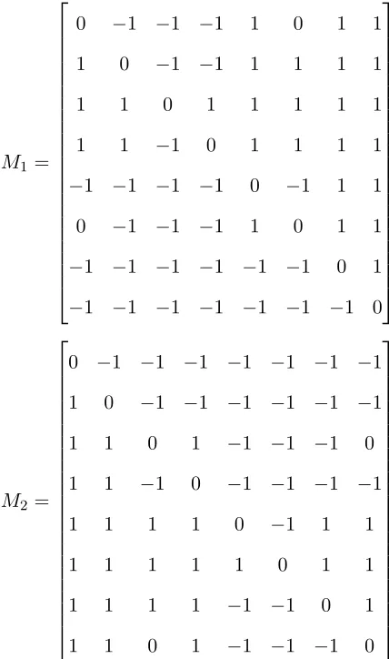
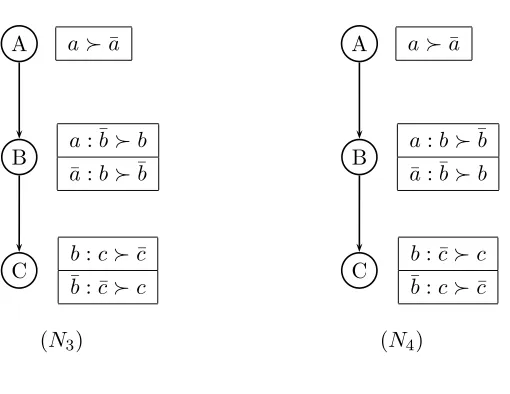
Example 1. LetN1, N2 ∈ NF be two CP-nets between which we intend to
mea-sure shared interest. For simplicity, we have defined N1 and N2 over the same feature set
F ={A, B, C}. That is, assume case 1 from Section 5.4 is satisfied. The two CP-nets are shown in Figure 6.1 annotated with their CPTs.
From the CPTs these two CP-nets we construct the respective preference orderings,
A
B
C
a≻¯a
a:b≻¯b
¯
a: ¯b≻b
b:c≻c¯ ¯b: ¯c≻c
(N1)
A
B
C ¯
a≻a
a:b≻¯b
¯
a: ¯b≻b
b:c≻c¯ ¯b: ¯c≻c
(N2)
Figure 6.1: Two CP-nets N1 andN2
M1 and M2 are shown below:
M1 =
0 −1 −1 −1 1 0 1 1
1 0 −1 −1 1 1 1 1
1 1 0 1 1 1 1 1
1 1 −1 0 1 1 1 1
−1 −1 −1 −1 0 −1 1 1
0 −1 −1 −1 1 0 1 1
−1 −1 −1 −1 −1 −1 0 1
−1 −1 −1 −1 −1 −1 −1 0
M2 =
0 −1 −1 −1 −1 −1 −1 −1
1 0 −1 −1 −1 −1 −1 −1
1 1 0 1 −1 −1 −1 0
1 1 −1 0 −1 −1 −1 −1
1 1 1 1 0 −1 1 1
1 1 1 1 1 0 1 1
1 1 1 1 −1 −1 0 1
1 1 0 1 −1 −1 −1 0
Now, the ith column vectors for M1 and M2 have corresponding labels. Once this has been done, the distance function defined earlier can be used to measure the sum of the
distances between each of the column vectors. In effect, the similarity of preference for the
outcome specified by the column label is being compared.
We use the distance function dΩ to sum over the distances of the preference rela-tions placed over each outcome, and divide by 2 to get the final distance measure. For our
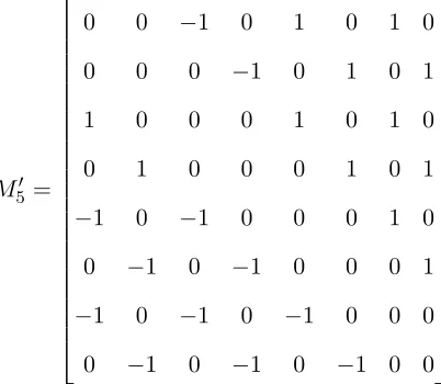
example CP-netsN1andN2, we find thatdΩ(ω1, ω2) = 30. This measure can be used now to compute the normalized shared interest function value. We note thatdΩmax =n(n−1) = 56, where n=|OF|= 8. We put this in our shared interest function I to get
I(N1, N2) = 1−
dΩ(ω1, ω2)
dΩ
max
= 1− 30
56 = 0.464 (6.9)
The example above is intended to provide an overview of the basic techniques being
used to make comparisons between the preference relations represented as CP-nets. This
is not meant to be a complete outline for the general problem of making interest matching
comparisons of CP-nets. Instead, we focused on a well-formed, ideal case which allowed us
to demonstrate these techniques and their basic properties without having to deal with the
problems associated with other cases. More general cases are discussed in Chapter 7.
6.5
CP-net Shared Interest Algorithm
In this section we state formally the CP-net Shared Interest Algorithm which is
used to compare two CP-nets and return a value indicating a level of shared interest. In
Ex-ample 1, we showed how the shared interest between two well-formed CP-nets is computed.
The algorithm is generalized in this section to account for all possible cases of CP-net
com-parisons outlined in Section 5.4.
The shared interest function takes two CP-nets N ∈ NF and N′ ∈ NF′ as input.
The restrictions stated in Section 5.3 are assumed to be true of the CP-nets. Using the CPTs, we construct the induced preference graph for each CP-net. Next, we check whether
the feature sets are the same for both CP-nets. Of course, it is possible that each set
possible combinations of binary feature values (instantiations) over the setV. We define the setOV, which contains all of these combinations. The preference graphP(N) for CP-netN
is extended so that it contains 2|V|disconnected graphs. Each of these disconnected graphs,
which we call Puk(N), is defined precisely as the original preference graph over OF except that each outcome oj ∈OF is now of the form ojuk, whereuk ∈OV and uk is unique for
each disconnected graphPuk(N). This same procedure is carried out if it is also determined
that |F −F′| ≥1.
The construction of the disconnected preference graphs is both a necessary and
sound modification of the original preference graph in order to preserve the flipping
se-quence semantics of the preference ordering it represents. Each of the disconnected
sub-graphs, Puk(N), maintains the preference ordering over the original set of outcomes. By
concatenating the same, unique instantiation of the differing features, the flipping sequence
remains legally defined. Furthermore, by removing the concatenated feature instantiations
from outcomes in Puk(N) we have preserved the original, unexpanded preference graph for N. The preservation of the stated preferences when constructing the expanded preference graph allows reliable comparisons to be made between significantly different CP-nets.
Once the preference graphs have been constructed properly, the ordering matrices
are constructed using the path-based method over the preference graphs as mentioned in
Section 6.1. The distance function dΩ is computed using these ordering matrices. The distance value along with the maximum possible distance, dΩmax, are used to compute the shared interest function, I(N, N′) = 1−dΩ(ω,ω′)
dΩ
Algorithm 1 CP-net Shared Interest Algorithm
1: Input: CP-netsN and N′
2: Output: Shared interest level between N and N′
3: Construct induced preference graphsP(N) and P(N′)
4: if |F′−F|>0 then
5: LetV =F′−F
6: ModifyP(N) to contain 2|V| disconnected preference graphs, call themPuk(N), such
that each Puk(N) is constructed over outcomes of the form ojuk for each oj ∈ OF,
whereuk ∈OV and uk is unique for each of the disconnected preference graphs.
7: end if
8: if |F−F′|>0 then
9: DefineV =F −F′
10: ModifyP(N′) to contain 2|V|disconnected preference graphs, call themPuk(N′), such
that each Puk(N′) is constructed over outcomes of the form ojuk for each oj ∈OF′,
whereuk ∈OV and uk is unique for each of the disconnected preference graphs.
11: end if
12: UsingP(N) and P(N′), construct ordering matrices M and M′ in canonical form
13: ComputedΩ(ω, ω′) using M and M′
14: Define dΩ
max usingn=|OF∪F′| 15: Return: I(N, N′) = 1−dΩ(ω,ω′)
dΩ
Chapter 7
CP-net Variations
The CP-nets used for comparisons will vary in topological structure or in CPT
specifications. In this chapter, we provide examples of some of these variations and discuss
how they influence the computation of shared interest level. An example is provided for
each of these properties along with an inline explanation of the results. It should be noted
that none of these variations require changes to the shared interest function. The discussion
of examples in this chapter provides the empirical evidence for motivating the structural
comparisons discussed in the next chapter.
7.1
Defining CP-net Permutations
We start by defining a simple method for permuting CP-nets through modifications
to the CPTs, which we call a CP-permutation. The construction of a CP-permutation
function is described below.
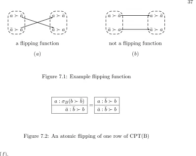
Let N ∈ NF be a fully-annotated CP-net. Let Pref(f) ={f ≻f ,¯ f¯≻f} be the
set of all possible preferences for featuref. As a step toward defining ourCP-permutation, we define a method for modifying CPTs in a CP-net. This is done using a flipping function
on a CPT row:
Definition A flipping function is the bijective function σf : Pref(f) → Pref(f) which
a≻¯a
¯
a≻a
a≻a¯
¯
a≻a
a flipping function
(a)
a≻¯a
¯
a≻a
a≻¯a
¯
a≻a
not a flipping function
(b)
Figure 7.1: Example flipping function
a:σB(b≻¯b)
¯
a: ¯b≻b =
a: ¯b≻b
¯
a: ¯b≻b
Figure 7.2: An atomic flipping of one row of CPT(B)
α ∈Pref(f).
Thus, in Figure 7.1 the flipping function (a) is a flipping function using the defi-nition provided above; however, (b) is not a flipping function. We use the flipping function to define a modification to a single row in a CPT, as well as a modification to the entire
CPT. These modifications are called an atomic flip and aCPT flip, respectively:
Definition Anatomic flip, oratomic flipping, is the application of the flipping functionσf
to a single row in CPT(f) for some f ∈F.
LetN ∈ NF be a CP-net, with F ={A, B}, such thatA∈P a(B) and Pref(B) =
{b≻¯b,¯b≻b}. LetσB be the flipping function defined for featureB. We say that an atomic
flipping σB has been applied to a row in CPT(B) when we modify, for example, the row a:b≻¯bto a: ¯b≻b. This modification of CPT(B) is depicted in Figure 7.2.
Definition A CPT flip, or CPT flipping, is the modification of each row in CPT(f) ac-cording to the flipping function σf. The function πf :NF → NF applies a single CPT flip to CPT(f) in a CP-net.
a:b≻¯b
¯
a: ¯b≻b
πB a:σB(b≻¯b)
¯
a:σB(¯b≻b) =
a: ¯b≻b
¯
a:b≻¯b
Figure 7.3: CPT-flipping functionπB
according to σB.
It is simple to note that the CPT flipping functionπf can be composed with other CPT flipping functions and applied to the same CP-net. Define aCP-permutation function Π =πfi◦. . .◦πfm as the composition of CPT flipping functions. If the restriction of Π to
feature f, denoted by Π↿f, is such that Π ↿f =πf, then we say that CPT(f) is flipped
in Π. Furthermore, if CPT(f) is not flipped in Π, then Π ↿ f = id, where id denotes the identity function, meaning that CPT(f) is unaffected by Π. ACP-permutation function Π and CPT flipping function πf are the same operationally when we have Π =πf (i.e., Π is composed of only one CPT flipping function).
Definition A CP-permutation function Π = πfi ◦ . . .◦πfm is the composition of CPT flipping functions πf.
A simple identity property Π(Π(N)) =N holds for the function Π. The identity definition follows intuition due to the nature of σf. By definition, the application of Π to a
CP-net N will result in a CP-net N′. Applying Π once again forN′ simply flips the CPTs back to the original CP-net N.
7.2
Relation between Shared Interest Values
The following example will expand on Example 1 by considering the relation of one
shared interest measure to another and discuss what is the relation to feature importance.
A level of relative feature importance is assigned through the explicit relation of the feature
nodes in the graph by interpretingfj ∈P a(fi) as meaning that featurefj is more important
to the user than fi. The purpose is to motivate what we mean when we say that an agent