HIGHLIGHTED ARTICLE INVESTIGATION
A General Uni
fi
ed Framework to Assess the
Sampling Variance of Heritability Estimates Using
Pedigree or Marker-Based Relationships
Peter M. Visscher*,†,1and Michael E. Goddard‡,§ *Queensland Brain Institute, University of Queensland, Brisbane, Queensland 4072, Australia†The University of Queensland Diamantina Institute, The Translational Research Institute, Brisbane, Queensland 4102, Australia,‡University of Melbourne, Department of Food and Agricultural Systems, Parkville, Victoria 3010, Australia, and§Biosciences Research Division, Department of Environment and Primary Industries, Bundoora, Victoria 3001, Australia
ABSTRACTHeritability is a population parameter of importance in evolution, plant and animal breeding, and human medical genetics. It can be estimated using pedigree designs and, more recently, using relationships estimated from markers. We derive the sampling variance of the estimate of heritability for a wide range of experimental designs, assuming that estimation is by maximum likelihood and that the resemblance between relatives is solely due to additive genetic variation. We show that well-known results for balanced designs are special cases of a more general unified framework. For pedigree designs, the sampling variance is inversely proportional to the variance of relationship in the pedigree and it is proportional to 1/N, whereas for population samples it is approximately proportional to 1/N2, whereN
is the sample size. Variation in relatedness is a key parameter in the quantification of the sampling variance of heritability. Consequently, the sampling variance is high for populations with large recent effective population size (e.g., humans) because this causes low variation in relationship. However, even using human population samples, low sampling variance is possible with highN.
H
ERITABILITY (h2), the proportion of phenotypic varia-tion that is explained by additive genetic variavaria-tion, is an important parameter in plant and animal breeding, evolution-ary genetics, and human and medical genetics. It is central in quantifying the role of genetics in complex traits, predicting response to selection in natural and artificial breeding pro-grams, and determining the limits of trait or disease pre-diction using information from relatives or DNA markers. Traditionally, the estimation of heritability is from pedigree data, by modeling the observed resemblance between rela-tives (Falconer and Mackay 1996; Lynch and Walsh 1998). More recently, genetic variation has been estimated using genetic marker information (Ritland 2000; Thomas 2005; Visscheret al.2006; Yanget al.2010; Robinsonet al.2013; Berenoset al.2014). These designs estimate the genetic var-iance explained by the markers, which may be less than the additive genetic variance (Yanget al.2010), but in this articlewe refer to the parameter estimated as the heritability re-gardless of whether it is estimated from relationships de-fined by pedigree or by markers. In general, designs to estimate heritability can be grouped by their use of (i) the expected identity-by-descent (IBD) sharing between relatives,
i.e., using pedigree relationships, (ii) marker-based estimated IBD relationships between relatives for known pedigree rela-tionships, and (iii) marker-based estimated genomic relation-ship matrices for unknown pedigree relationrelation-ships. For a review of these designs with a particular focus on human populations, see Vinkhuyzenet al.(2013).
Even with large sample sizes, the standard error of heri-tability estimates is often disappointingly large and it varies greatly between experimental designs. Therefore it is impor-tant to calculate the expected standard error before com-mitting resources to collecting the data. Given a particular experimental design and the population value of h2, its sampling variance can be determined using a number of methods. After the data have been collected, the (asymptotic) sampling variance of the estimate can be derived from the analysis, for example, from mean squares in balanced de-signs, from the information matrix when using maximum likelihood or from the posterior density in Bayesian analysis.
Copyright © 2015 by the Genetics Society of America doi: 10.1534/genetics.114.171017
Manuscript received September 17, 2014; accepted for publication October 27, 2014; published Early Online October 31, 2014.
Available freely online through the author-supported open access option.
Prior to collecting data on phenotypes, the sampling vari-ance can be predicted using statistical theory, typically for balanced designs, or obtained from computer simulation for more complex pedigree structures. In this study, we provide a single framework for calculating the asymptotic sampling variance of the heritability across a wide range of designs, for a class of models with two random variables and when analysis is by maximum likelihood (ML). We derive the sampling variance using the expected value of the information matrix. We show that previous results are special cases of the general framework and that the vari-ance in relationships in the sample is a key parameter in all experimental designs.
Model and Assumptions
We assume a linear model with no fixed effects (orfixed effects that have been adjusted for without error) and two random components, a genetic effect (g), and a residual ef-fect (e). There areNindividuals, each with a single obser-vation,y,
y¼gþe; with varðgÞ ¼Gs2g and varðeÞ ¼Is2e;
wherey,g, andeare vectors of lengthNof the phenotypic observations, genetic value, and residuals, respectively.Gis the genetic relationship matrix (GRM), either from pedigree relationships, in which case it is the usual numerator rela-tionship matrix (twice the kinship matrix), or derived from SNP similarity (Vanraden 2008; Stranden and Garrick 2009; Yanget al.2010). The genetic, residual, and total variances are sg2, se2, and s2, respectively. The N 3 N covariance matrix of all observations (V) is
varðyÞ ¼V¼Gh2þI12h2s2;
whereh2=s
g2/(sg2+se2) =sg2/s2, the heritability.
General Formula for Sampling Variance
We can decompose the symmetric GRM as
G¼TDT9;
with TT9=T9T =IandT21=T9becauseT is orthogonal and D a diagonal matrix containing eigenvalues (li) of G. Inference onh2from dataydoes not change upon a linear transformation ofy. We can therefore transformyby using the eigenvectors ofG, which for the simple model used here are also eigenvectors of V (Thompson and Shaw 1990, 1992; Lippert et al. 2011; Blangeroet al. 2013; Raffa and Thompson 2014).
Define y*¼T21y¼T9y: Then
y*¼T9gþT9e¼g*þe*;
with
varðy*Þ ¼P¼ h
T9GTh2þT9T
12h2is2
¼Dh2þI12h2s2:
The log likelihood with respect toh2ands2is
logL¼ 21
2
h
logjPj þy*9P21y*i
¼ 21
2
h
N3logs2þXloglih2þ12h2
þ1s2S
y*2 i
.
lih2þ12h2i;
(1)
as shown previously (Thompson and Shaw 1990; Raffa and Thompson 2014). Equation 1 is very similar to that in Blangero et al.(2013), but with added parameters2. Ele-ments of the (Fisher) information matrix (F) are obtained by taking the second derivative of (1) taken at the maximum with respect toh2ands2, and then the negative value of its expectation overy*, using
E
y*2i
¼var
y*i
¼lih2þ12h2s2 ¼1þh2ðli21Þs2:
The derivation of thefirst element ofF(F11) is given here. The other two elements are derived analogously,
dlogLdh2¼ 21
2
h X
ðli21Þlih2þ12h2
21s2S
y*2 i ðli21Þ
.
lih2þ12h22
i
dlogL2dh4¼ 21
2
h
2Xðli21Þ2.lih2þ12h22
þ21s2S
y*2 i ðli21Þ
2.
lih2þ12h23
i
and so
F11¼ 2EdlogL2dh4
¼1
2
Xh
2ðli21Þ2.1þh2ðli21Þ2
i
þ2ðli21Þ2.1þh2ðli21Þ2
i
¼1
2
Xh
ðli21Þ2.1þh2ðli21Þ2i:
The resulting elements of the 2 3 2 matrix F areF11¼12a; F12¼F21¼21b=s2; F22¼12N=s4;with con-stants aandb,
a¼Xhðli21Þ2.1þh2ðli21Þ2
i ;
and
These elements are similar to those presented in Thompson and Atkins (1994), who parameterized the likelihood in a genetic and residual variance component, whereas we have parameterized in heritability and phenotypic variance. Thompson and Atkins do not have the factor1
2and haveli2 andliin the equations above where we have (li–1)2and (li – 1), respectively, the difference due to the choice of parameters in the model. In the article that developed the method of estimation of variance component in linear mixed models using restricted maximum likelihood (Patterson and Thompson 1971), the authors presented both the log likeli-hood and the information matrix in terms of eigenvalues of the covariance matrix.
The asymptotic sampling (co)variance for the estimates of heritability and phenotypic variance are fromF21. There-fore, the asymptotic sampling variance of the estimate of the heritability is
var
^
h2
2a2b2N: (2)
Hence, under the assumptions given, this is a completely general expression for the asymptotic sampling variance of an estimate of heritability and depends only on the eigenvalues of the GRM, the population value of heritability, and the experimental sample size.
Special Cases
With additional assumptions or for balanced designs, terms for a and bsimplify and simple solutions for the sampling variance of ^h2 can be derived. We go through a number of these special cases in this section that encompass pedigree and marker-based GRM.
Phenotypic variance (s2) known
In many applications, the sampling variance of the total phenotypic variance is small or known before the experiment is conducted, and therefore it is useful to consider the sampling variance of heritability under the assumption that the pheno-typic variance is known without error. For example, Blangero
et al.(2013) assume thats2is known in their derivations of the expected likelihood-ratio-test statistic (ELRT). If we assume here that the phenotypic variance is known without error then the resulting sampling variance of the estimate of heritability is
var
^
h2 s2 known
¼2=a: (3)
This expression is smaller than that in (2); hence assuming that phenotypic variance is known when it is not will lead to an underestimate of the sampling variance of heritability. This underestimate will be small whenb2/Nis small relative to the terma.
h2/0
For a small heritability,a /Pðli21Þ2;b /Pðli2 NÞ;
and
var^h2 h2/02.½N3varðliÞ: (4)
Assuming that the phenotypic variance is known and h2 is small gives
var
^
h2 s2 known;h2/0
2
.h
N3varðliÞ
þNðEðliÞ21Þ2
i ;
which is close to (4) because the mean eigenvalue will be 1 in the absence of inbreeding when the GRM is from pedigree identity-by-descent and very close to 1 when the GRM is estimated from SNP data (Jansset al.2012). Hence, when the population value of heritability is small, its sampling variance is only a function of the variation in relatedness and sample size.
Allli/1
Equation 4 is also the result for when allliare close to 1, such that their variance approaches zero. This situation can occur when the GRM is created from population SNP data on unre-lated individuals in a population with a large effective population size. However, as we derive below, the variance of eigenvalues depends both on experimental sample size and effective pop-ulation size, and so these parameters affect the sampling var-iance of heritability. In particular, the varvar-iance in eigenvalues is proportional to experimental sample size, so the larger the sample size the wider the spread around a mean value of 1.
Pairs of relatives with relationship r
If there arempairs of relatives of the same degreer, then 2m=Nand there aremeigenvaluesl1with value 1 +rand
m eigenvaluel2 with value 12r(Searle 1982; Blangero
et al.2013). Letr=rh2. Then
a¼2mr21þr2h4.12r2h42
¼2mr21þr2.12r22;
b¼22mr2h212r2h4¼22mrr12r2;
and
var^h2¼12r22.mr2: (5)
For pairs of monozygotic (MZ) twins (r = 1), Equation 5 becomes var(h^2) = (1–r2)2/m. For pairs of full-sibs (r=1
2), the sampling variance is 4(1–r2)2/m. For bivariate normality, the sampling variance of a correlation coefficient between two variates with population valueris(1–r2)2/N(e.g., Lynch and Walsh 1998, p. 819), so consistent with Equation 5.
Balanced design of multiple families
per family. This follows from known results on eigenvalues for symmetrical matrices that can be written as cI+dJ, with c
anddconstants (Searle 1982). Substituting these eigenvalues into the equation for parametersaandbgives
a¼m r2 nðn21Þ1þr2ðn21Þ.hð12rÞ2ð1þ ðn21ÞrÞ
i2
b¼2mnðn21Þrr=½ð12rÞð1þrðn21ÞÞ
and
var^h22ð12rÞ2½1þ ðn21Þr2.mnðn21Þr2: (6)
This is consistent with the intraclass correlation sampling variance (e.g., Falconer and Mackay 1996, p. 180), apart from havingmin the denominator [the least-squares deri-vation has (m21) instead]. Although we have assumed no fixed effects, in practice at least a mean would be included in the model and this absorbs one degree of freedom from the comparison of families. The least-squares formula takes account of this but ML estimation ignores it. Assuming that the phenotypic variance is known gives
var
^
h2
2ð12rÞ2½1þ ðn21Þr2.mnðn21Þr2
31þr2ðn21Þ;
smaller than (5) by a factor of 1/(1 +r2(n21)). For large half-sib families, this term can be substantial.
Twin design
In human populations, the classical twin design is common for estimating genetic and nongenetic variance components. LetN= 2mM + 2mD, with mM andmDthe number of MZ and dizygotic (DZ) pairs, respectively. In total, there are four different eigenvalues: 2, 0, 3/2, and 1/2 (Blangero et al.
2013), with multiplicity mM, mM, mD, and mD. Let c =
mM/(mM +mD), the proportion of all twin pairs that are MZ pairs. Using Equation 5,a2b2/N=NT, with
T¼c1þh4ð12cÞ.12h42
þ1
4ð12cÞ
1þ1 4h
4 c
,
121 4h
4 2
21
4cð12cÞh
412h4121
4h
4
and
var
^
h2
¼ ð2=NÞT21:
This analysis assumes that there are no common environ-mental effects so the sampling variance is not appropriate for the usual practice of estimation of heritability using maxi-mum likelihoodfitting both an additive genetic and common environmental component (Neale and Cardon 1992).
Within-family estimation using realized relationships estimates from markers
Full-sibs have an expected pedigree relationship of 0.5 but the actual amount of the genome shared varies around 0.5 and this realized relationship can be estimated using genetic markers and used to estimate heritability (Visscher et al.
2006, 2007; Hemani et al. 2013). These relationships can be estimated using identity-by-descent calculations con-ditional on observed marker genotypes. For full-sibs and half-sibs in human populations, the standard deviation of realized relationships is 0.04 and 0.03, around the expected value of1
2and
1
4, respectively. For a comprehensive theory on the variance of realized relationships, see Hill and Weir (2011). A feature of this design is that common envi-ronmental factors that vary between families do not bias the heritability estimate. Visscher et al. (2006) derived an ap-proximate sampling variance of the estimate of heritability from multiple families with two full-sibs each. Hill (2013) derived the sampling variance of the estimate of genetic variation using REML for the general case offfamilies each of sizenand expected relationshipu(twice the kinship co-efficient). We can use the same general framework as de-veloped here to approximate the sampling variance from within-family estimation. The difference between this de-sign and those previously discussed is that the GRM is not fixed. That is, the eigenvalues of the GRM are themselves random variables and to derive the sampling variance of the estimate of heritability we need tofirst derive the expected value of the elements of the Information matrix over re-peated samples. We provide details of an approximation in
Appendix A. It results in
var
^
h2
h2ð12tÞ2
.
f3n2*varriji
3hð12tÞ22nh4varrij i
¼h2ð12tÞ2.Nn3varrij i
3hð12tÞ22nh4varriji:
(7)
This equation shows that the sampling variance reduces by the square of the sample size per family (n), essentially because every individual adds a contrast with all other family members in the sample. As detailed in Appendix A, this ap-proximation breaks down whenh2andnare large.
Random sampling from the population
distantly, because the population size isfinite. In human pop-ulations, this sampling scheme corresponds to sampling indi-viduals who are conventionally unrelated. As for the case of realized relationships within families, the GRM is not fixed. We approximateE(a) andE(b2) inAppendix B. The resulting sampling variance of the estimate of heritability is
var^h22EðaÞ2Eb2N¼2N2 vðuÞ; (8)
wherev(u) is the variance of relatedness in the population, which is a function of effective population size (Goddard 2009; Goddardet al.2011). Analogous to the within-family design, the sampling variance is inversely proportional to the square of the sample size, rather than by 1/Nin pedigree designs. Rijsdijk and Sham (2002) derived the same result (parameterized as the noncentrality-parameter, NCP, of the test statistic for heritability) for QTL linkage mapping in pedigrees, assuming that the variance in relatedness is small. Equation 8 was previously derived for SNP-based es-timation of variance components from linear regression the-ory, assuming that the phenotypic variance is known without error (Vinkhuyzenet al.2013; Visscheret al.2014).
Statistical Power
The interest in this study is not about hypothesis testing but about quantifying the sampling variance of the estimate of heritability. For a detailed treatment on statistical power in variance component estimation using (restricted) maximum likelihood we refer to previous publications (Self and Liang 1987; Shaw 1987; Thompson and Shaw 1990; Almasy and Blangero 1998; Williams and Blangero 1999; Rijsdijket al.
2001; Purcellet al.2003; Raffa and Thompson 2014). Here we briefly consider the expected value of two test statistics that have been used for hypothesis testing in variance compo-nent estimation, the Wald test, and the likelihood-ratio-test statistic.
The Wald test is based on ^h4/var(^h2), which under the null hypothesis thath2= 0, follows ax2distribution. How-ever, ifh2.0, the Wald test statistic follows approximately a noncentralx2with noncentrality parameter (NCP
W)
NCPW¼h4 .
var
^
h2
¼1
2h
4a2b2N
¼1
2h
4 Xhðli21Þ2.
1þh2ðli21Þ2
i
2 Xðli21Þ 1þh2ðli21Þ2.N
:
(9)
If the estimation of phenotypic variance is ignored, then
NCPW¼1
2h
4 a¼1
2h
4 "
Xh
ðli21Þ2.1þh2ðli21Þ2
# :
(10)
Alternatively, the null hypothesis thath2= 0 can be tested with a likelihood-ratio test. Blangero and colleagues (Blangero
et al. 2013) presented a very simple equation for the ELRT statistic to test the null hypothesis ofh2= 0,
NCPLRT¼ 2 X
ln1þh2ðli21Þ: (11)
Equation 11 converges to Equation 10 whenh2(l
i21)/
0. For pairs of relatives with relationshipr, NCPW=12Nr2h4/ (1– r2h4) and NCP
LRT=212Nln(12r2h4). These expres-sions are equivalent whenr2h4/0. When the true param-eter is far from the one being tested under the null, these expressions can give quite different values. Raffa and Thompson (2014) give an analysis based on asymmetrical confidence intervals for the heritability.
Numerical Examples
Figure 1 shows the approximation to the standard error of an estimate of heritability as a function of the population value, experimental sample size, and design. Four different designs were used: a pedigree design of unrelated full-sib pairs, a pedigree design with MZ and DZ twins pairs with a ratio of 1:2 MZ and DZ pairs, a within-family design using full-sib pairs, and a population design using nominally un-related individuals. In the last two designs, GRM are esti-mated with SNP data. These designs are less powerful than the pedigree-based experimental designs, but make fewer assumptions. At N= 10,000 the sampling variance of the population design approaches that of the pedigree designs, and at N= 100,000 it becomes the most powerful design. Sample sizes of 100,000 are realistic in human population and even larger samples sizes are expected in the next few years. Therefore, strong inference on heritability can be drawn using random samples from the population, while not having to make assumptions about the resemblance be-tween relatives due to common environmental factors. The within-family design, which is the most robust with respect to assumptions of the model, remains inaccurate even when the analysis is on 50,000 full-sib pairs. However, in species such asfish with huge full-sib family sizes, accurate estima-tion could be achieved (Odegard and Meuwissen 2012; Hill 2013).
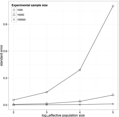
Figure 2 shows results for the population design for spe-cies with differentNevalues of 1000, 10,000, and 100,000. It shows the increase in sampling variation with increasing effective population size, which is due to the decrease in the variation in relatedness. For the within-family design the sampling variance of heritability does not depend on the ef-fective population size.
Discussion
Figure 1 shows that the sampling variance is relatively in-sensitive to the true value ofh2except whenh2/1. The results recapitulate results from balanced designs and show that for pedigree designs, the sampling variance tends to be proportional to 1/N. In contrast, for designs that use genetic markers to estimate relatedness within families or estimate relatedness among randomly sampled individuals, the sam-pling variance is proportional to 1/N2. Consequently, very large samples of “unrelated” individuals are powerful for estimating h2. The key feature of the experimental design is the variation in relatedness. This is small within families of full-sibs and consequently the sampling variance ofh2is large.
There are a number of limitations to our study. First, we have assumed that the parameter whose sampling variance we derive is the same in different experimental designs. Even in the absence of confounding factors such as common environmental effect or nonadditive genetic factors, this is not necessarily the case. For the pedigree and within-family design, the parameter given our model assumptions is the narrow-sense heritability. But for the population design it is the proportion of phenotypic variance captured by genetic markers. If these markers are not sufficiently correlated with the genetic variants that cumulatively contribute to the total
narrow sense heritability, then the use of a marker-based GRM will estimate additive genetic variation that is less than the total additive genetic variance. This can occur if the properties of the markers used to create the GRM are dif-ferent from the segregating causal variants, for example, if the GRM is based upon common SNPs and the causal variants have lower heterozygosity, leading to loss of information due to imperfect linkage disequilibrium (Yang et al. 2010). Al-though a“marker heritability”is conditional on the markers used to estimate relatedness, it is a valid population param-eter with predictable sampling properties (as shown in this study). In human populations, it has been used to address the question of“missing heritability”from genome-wide associa-tion studies (Yanget al.2010).
Second, we assume that all resemblance between rela-tives is due to additive genetic covariance, so that there are only two random effects in the model. Additional random effects, for example, common environmental effects, make the covariance matrixVmore complicated and generally not diagonalizable. When there are additional variance compo-nents, the residual variance as used in this study is partitioned in two or more components. These additional components are also estimated with error and will have a sampling co-variance with the estimate of heritability. We suspect that
Figure 1 Standard error of estimates of
having additional variance components in the model will tend to increase the sampling variance of the heritability, except for some balanced designs. However, we have not investigated general properties for designs with multiple random effects. With more than two variance components, computer simulation might be an efficient way to quantify the sampling variance of heritability and the proportion of variance due to additional random effects.
A third assumption is that estimation is by maximum likelihood or, alternatively, thatfixed effects and covariates have been adjusted for without error. In practice, research-ers tend to use least squares for balanced designs and restricted maximum likelihood (REML) or Bayesian meth-ods for unbalanced designs. The difference in sampling variance between ML and REML is small when there are few fixed effects relative to the sample size, as, for example, in human genetic applications, but larger in situations where there are manyfixed effects (e.g., in livestock applications). Recently, Raffa and Thompson (2014) extended the work of Blangeroet al.(2013) by deriving approximations to the ELRT and confidence intervals of the heritability estimate using Taylor series expansions of the expected likelihood-ratio test with respect to the distribution of the eigenvalues of a given pedigree. Their simplest approximation can be expressed as an approximate sampling variance of the esti-mate of heritability as 2/[(N21)var(l)] 2/(Nvar(l)). This expression is the same as our special casesh2/0 and
All li/1. The authors show that this approximation is not accurate when the assumptions break down, in particular when eigenvalues are not closely distributed around the
mean of 1, and provide a better approximation using the logarithm of the eigenvalues (Raffa and Thompson 2014). They also show that confidence intervals of the estimates of heritability are not symmetrical when the variance in eigen-values is large and that Wald statistic-based confidence intervals can be too narrow, implying that the use of the derived standard errors in our study to construct a confi -dence interval can be anticonservative. Although the deriva-tions from Raffa and Thompson were for a pedigree design, they should also apply to other experimental designs, such as those where GRMs are estimated from marker data.
In conclusion, we have proposed a general unified frame-work to assess the sampling variance of the estimate of heritability using pedigree or marker-based relationships and have quantified how the sampling variance depends on sample size and the variation in relatedness.
Acknowledgments
This study was inspired by John Blangero’s presentation at the 2013 Statistical and Quantitative Genetics conference in Seattle. We thank Bill Hill for discussions and helpful com-ments, Jesse Raffa for useful comcom-ments, and Matt Robinson and Kostya Shakhbazov for feedback and help with R. This research was supported by U.S. National Institutes of Health (NIH) grant R01 GM075091.
Literature Cited
Almasy, L., and J. Blangero, 1998 Multipoint quantitative-trait linkage analysis in general pedigrees. Am. J. Hum. Genet. 62: 1198–1211.
Berenos, C., P. A. Ellis, J. G. Pilkington, and J. M. Pemberton, 2014 Estimating quantitative genetic parameters in wild pop-ulations: a comparison of pedigree and genomic approaches. Mol. Ecol. 23: 3434–3451
Blangero, J., V. P. Diego, T. D. Dyer, M. Almeida, J. Peraltaet al., 2013 A kernel of truth: statistical advances in polygenic variance component models for complex human pedigrees. Adv. Genet. 81 (81): 1–31.
Falconer, D. S., and T. F. C. Mackay, 1996 Introduction to Quan-titative Genetics. Longman, Harlow, Essex, United Kingdom. Goddard, M., 2009 Genomic selection: prediction of accuracy and
maximisation of long term response. Genetica 136: 245–257. Goddard, M. E., B. J. Hayes, and T. H. Meuwissen, 2011 Using the
genomic relationship matrix to predict the accuracy of genomic selection. J. Anim. Breed. Genet. 128: 409–421.
Hemani, G., J. Yang, A. Vinkhuyzen, J. E. Powell, G. Willemsen et al., 2013 Inference of the genetic architecture underlying BMI and height with the use of 20,240 sibling pairs. Am. J. Hum. Genet. 93: 865–875.
Hill, W. G., 2013 On estimation of genetic variance within fami-lies using genome-wide identity-by-descent sharing. Genet. Sel. Evol. 45: 32.
Hill, W. G., and B. S. Weir, 2011 Variation in actual relationship as a consequence of Mendelian sampling and linkage. Genet. Res. 93: 47–64.
Janss, L., G. de Los Campos, N. Sheehan, and D. Sorensen, 2012 Inferences from genomic models in stratified populations. Genetics 192: 693–704.
Figure 2 Standard error of the estimate of heritability from random
Lippert, C., J. Listgarten, Y. Liu, C. M. Kadie, R. I. Davidsonet al., 2011 FaST linear mixed models for genome-wide association studies. Nat. Methods 8: 833–835.
Lynch, M., and B. Walsh, 1998 Genetics and Analysis of Quantita-tive Traits. Sinauer, Sunderland, MA.
Neale, M., and L. R. Cardon, 1992 Methodology for Genetic Studies of Twins and Families. Kluwer, Dordrecht, The Netherlands. Odegard, J., and T. H. Meuwissen, 2012 Estimation of heritability
from limited family data using genome-wide identity-by-descent sharing. Genet. Sel. Evol. 44: 16.
Patterson, H. D., and R. Thompson, 1971 Recovery of interblock information when block sizes are unequal. Biometrika 58: 545– 554.
Purcell, S., S. S. Cherny, and P. C. Sham, 2003 Genetic Power Calculator: design of linkage and association genetic mapping studies of complex traits. Bioinformatics 19: 149–150. Raffa, J. D., and E. A. Thompson, 2014 Power and efffective study
size based on approximations to the expected likelihood ratio test in heritability studies. Department of Statistics, University of Washington, Technical Report #630. Available at:http://www. stat.washington.edu/research/reports/2014/tr630.pdf
Rijsdijk, F. V., and P. C. Sham, 2002 Analytic approaches to twin data using structural equation models. Brief. Bioinform. 3: 119– 133.
Rijsdijk, F. V., J. K. Hewitt, and P. C. Sham, 2001 Analytic power calculation for QTL linkage analysis of small pedigrees. Eur. J. Hum. Genet. 9: 335–340.
Ritland, K., 2000 Marker-inferred relatedness as a tool for detect-ing heritability in nature. Mol. Ecol. 9: 1195–1204.
Robinson, M. R., A. W. Santure, I. Decauwer, B. C. Sheldon, and J. Slate, 2013 Partitioning of genetic variation across the ge-nome using multimarker methods in a wild bird population. Mol. Ecol. 22: 3963–3980.
Searle, S. R., 1982 Matrix Algebra Useful for Statistics. Wiley, New York.
Self, S. G., and K. Y. Liang, 1987 Asymptotic properties of maximum-likelihood estimators and maximum-likelihood ratio tests under nonstandard conditions. J. Am. Stat. Assoc. 82: 605–610.
Shaw, R. G., 1987 Maximum-likelihood approaches applied
to quantitative genetics of natural-populations. Evolution 41: 812–826.
Stranden, I., and D. J. Garrick, 2009 Technical note: derivation of equivalent computing algorithms for genomic predictions and reliabilities of animal merit. J. Dairy Sci. 92: 2971–2975. Thomas, S. C., 2005 The estimation of genetic relationships using
molecular markers and their efficiency in estimating heritability in natural populations. Philos. Trans. R. Soc. Lond. B Biol. Sci. 360: 1457–1467.
Thompson, E. A., and R. G. Shaw, 1990 Pedigree analysis for
quantitative traits: variance-components without matrix-inver-sion. Biometrics 46: 399–413.
Thompson, E. A., and R. G. Shaw, 1992 Estimating polygenic
models for multivariate data on large pedigrees. Genetics 131: 971–978.
Thompson, R., and K. D. Atkins, 1994 Sources of information for estimating heritability from selection experiments. Genet. Res. 63: 49–55.
VanRaden, P. M., 2008 Efficient methods to compute genomic
predictions. J. Dairy Sci. 91: 4414–4423.
Vinkhuyzen, A. A., N. R. Wray, J. Yang, M. E. Goddard, and P. M. Visscher, 2013 Estimation and partition of heritability in hu-man populations using whole-genome analysis methods. Annu. Rev. Genet. 47: 75–95.
Visscher, P. M., S. E. Medland, M. A. Ferreira, K. I. Morley, G. Zhu et al., 2006 Assumption-free estimation of heritability from genome-wide identity-by-descent sharing between full siblings. PLoS Genet. 2: e41.
Visscher, P. M., S. Macgregor, B. Benyamin, G. Zhu, S. Gordonet al., 2007 Genome partitioning of genetic variation for height from 11,214 sibling pairs. Am. J. Hum. Genet. 81: 1104–1110. Visscher, P. M., G. Hemani, A. A. Vinkhuyzen, G. B. Chen, S. H. Lee
et al., 2014 Statistical power to detect genetic (co)variance of complex traits using SNP data in unrelated samples. PLoS Genet. 10: e1004269.
Williams, J. T., and J. Blangero, 1999 Power of variance compo-nent linkage analysis to detect quantitative trait loci. Ann. Hum. Genet. 63: 545–563.
Yang, J., B. Benyamin, B. P. McEvoy, S. Gordon, A. K. Henderset al., 2010 Common SNPs explain a large proportion of the herita-bility for human height. Nat. Genet. 42: 565–569.
Appendix A: Derivation of the Sampling Variance of Heritability from Within-Family Designs
As before,y=g+e, with var(g) =Gsg2and var(e) =Ise2. If all individuals belong to a family,E(G) =Ion diagonals andu on off-diagonals. We extract the family mean (u) from an individual’s breeding value soy=u+g* +e, where var(g*) = (G2uJ)sg2=Wsg2. If we treatuasfixed, then var(y2u) =Wsg2+Ise2. The mean eigenvalue ofWis (12u) and the variance of eigenvalues isn3var(rij) whererijis the realized relationship between individualsiandjwithin the same family. As in Hill(2013), we derive the sampling variance for a single family of size n. Under our assumed model of no environmental effects shared by family members,t=uh2. As before, the elements of the information matrix areF
11= 1/
2a,F12=F21=12b/s2,F22=12n/s4. We approximate the elements of the information matrix by taking a second-order Taylor series about the mean eigenvalue of (12u). Then, approximately,
EðaÞ=n¼u2 .
ð12tÞ2þ1þ2uh2n3varrij.ð12tÞ4
EðbÞ=n¼2u.ð12tÞ2h2n3varrij .
ð12tÞ3:
Using these to construct the (F21)1,1gives
varh2 h
2ð12tÞ2.n23varrijihð12tÞ22nh4varriji:
Using this approximation, the determinant of the information matrix, and therefore the approximation of the sampling variance of heritability, can be negative, whenn.(12t)2/(h43var(rij)). For example, for full-sibs (var(rij)0.0382) and
h2= 0.8 (andt= 0.4), a sampling size ofn= 390 full-sibs would result in a predicted sampling variance of the estimate of heritability that is negative. Presumably a higher-order Taylor series would correct this, but at the expense of having a relatively simple expression.
If we now use the eigenvalue decomposition ofW, as in Thompson and Atkins (1994) and as used in our other designs but parameterizing the variance components instead of h2 ands2, then the element of the Information matrix (Sin the Hill notation) are
S11¼1
2a¼ 1 2
X l2i
s2eþlis2g 2
;
S12¼1
2b¼ 1 2
X li
s2eþlis2g 2
;
S22¼1
2c¼ 1 2
X
1s2eþlis2g 2
:
If we take expectations ofa,b, andc, where the expectation is over the eigenvalues ofW[with mean = (12u), variance = var(l)n3var(rij)], then, from a second-order Taylor series about the mean:
EðaÞ=n¼ ð12uÞ2
.
ð12tÞ2þ
h
varðlÞ
.
ð12tÞ4ih12h2222ð12uÞh212h2i;
EðbÞ=n¼ ð12uÞ.ð12tÞ2þhvarðlÞ.ð12tÞ4ið12uÞh422h212h2;
EðcÞ=n¼1
.
ð12tÞ2þ
h
varðlÞ
.
ð12tÞ4i3h4:
Finally, the sampling variance of the estimate ofsg2is, approximately,
vs2g
h2ð12tÞ2.ðn3varðlÞÞihð12tÞ2þ3h4varðlÞi.hð12tÞ2þ 2h4varðlÞi
¼h2ð12tÞ2.n2varrijihð12tÞ2þ3nh4varriji.hð12tÞ22nh4varriji:
Appendix B: Derivation ofE(a) andE(b) for Population Designs
Letxi=li21, so thata=Sxi2/ (1 +xih2)2], andb=Sxi/ (1 +xih2). A second-order Taylor series expansion aroundx/ 0 givesE(a) =Nvar(l) andE(b2) =E(a).
The variance of eigenvalues is derived from the GRM (G)
G¼TDT9
with diagonal matrixDcontaining the eigenvaluesl.Gcan also be written as
G¼IþD;
withIthe identify matrix andDa matrix containing small relationships between distantly related individuals. ElementDijare
random with E(Dij) = 0 and var(Dij) =v(u), the variance in relatedness in the population.v(u) is a function of effective
population size (Goddard 2009; Goddardet al.2011),
G2¼TD2T9
trG2¼Xl2i ¼N½1þvarðlÞ; since EðlÞ ¼1
G2¼ ½IþD2¼Iþ
2 DþD2;
with
trG2¼Nþ0þtrD2¼NþN2 vðuÞ;
since tr(D2) is the sum of squares of element inD, each with expectationv(u).
Hence, we haveE(a) =E(b2) =Nvar(l) =N2v(u). Therefore, var(l) =Nv(u) and proportional to experimental sample size. Finally,
varh22EðaÞ2Eb2N¼2=½EðaÞð121=NÞ 2=EðaÞ ¼2N2 vðuÞ: