HIGHLIGHTED ARTICLE
GENETICS | INVESTIGATION
Bayesian Network Reconstruction Using Systems
Genetics Data: Comparison of MCMC Methods
Shinya Tasaki,*,1Ben Sauerwine,†Bruce Hoff,‡Hiroyoshi Toyoshiba,* Chris Gaiteri,‡,§,**,1,2
and Elias Chaibub Neto‡,1,2
*Integrated Technology Research Laboratory, Pharmaceutical Research Division, Takeda Pharmaceutical Company, Fujisawa, Kanagawa, Japan 251-8555,†Google, Seattle, Washington 98103,‡Sage Bionetworks, Seattle, Washington 98109,§Modeling, Analysis, and Theory Group, Allen Institute for Brain Science, Seattle, Washington 98103, and **Rush Alzheimer’s Disease Center, Rush University Medical Center, Chicago, Illinois 60612
ABSTRACTReconstructing biological networks using high-throughput technologies has the potential to produce condition-specific interactomes. But are these reconstructed networks a reliable source of biological interactions? Do some network inference methods offer dramatically improved performance on certain types of networks? To facilitate the use of network inference methods in systems biology, we report a large-scale simulation study comparing the ability of Markov chain Monte Carlo (MCMC) samplers to reverse engineer Bayesian networks. The MCMC samplers we investigated included foundational and state-of-the-art Metropolis–Hastings and Gibbs sampling approaches, as well as novel samplers we have designed. To enable a comprehensive comparison, we simulated gene expression and genetics data from known network structures under a range of biologically plausible scenarios. We examine the overall quality of network inference via different methods, as well as how their performance is affected by network characteristics. Our simulations reveal that network size, edge density, and strength of gene-to-gene signaling are major parameters that differentiate the performance of various samplers. Specifically, more recent samplers including our novel methods outperform traditional samplers for highly interconnected large networks with strong gene-to-gene signaling. Our newly developed samplers show comparable or superior performance to the top existing methods. Moreover, this performance gain is strongest in networks with biologically oriented topology, which indicates that our novel samplers are suitable for inferring biological networks. The performance of MCMC samplers in this simulation framework can guide the choice of methods for network reconstruction using systems genetics data.
KEYWORDSBayesian networks; MCMC methods; causal inference; eSNPs; network reconstruction
C
OMPLEX diseases such as Alzheimer’s disease and type 2 diabetes are influenced by intricate gene-to-gene and gene-by-environment interactions (Peilaet al.2002; Huang et al.2005; Liuet al.2007; Rhinn et al.2013). The goal of gene network reverse engineering is to learn the gene-to-gene interaction architecture underlying such diseases. Some algo-rithms output networks that correspond to putative causalrelationships among genes, by combining SNP and expression data. These inferred networks can be used to generate hypoth-eses that can be validated experimentally (Schadtet al.2005; Chenet al.2007; Atenet al.2008; Ferraraet al.2008; Chaibub Netoet al.2008, 2013; Duarte and Zeng 2011). In particular, Bayesian approaches to inferring causal networks are becom-ing a common practice in the field of systems biology (Zhu et al.2007, 2008; Chaibub Neto et al.2010; Hagemanet al. 2011; Moonet al.2014) and have successfully generated novel insights into biological processes (Zhanget al.2013). Nonethe-less, inferring the structure of Bayesian networks remains a challenging statistical and computational problem. Specifi-cally, the relative performance of different causal network re-construction algorithms is unclear when they are applied to real biological data sets. Therefore, to enable more accurate network reconstructions, we conduct a systematic comparison of the performance of several Markov chain Monte Carlo
Copyright © 2015 by the Genetics Society of America doi: 10.1534/genetics.114.172619
Manuscript received December 14, 2014; accepted for publication January 26, 2015; published Early Online January 28, 2015.
Available freely online through the author-supported open access option.
Supporting information is available online athttp://www.genetics.org/lookup/suppl/ doi:10.1534/genetics.114.172619/-/DC1.
1Corresponding authors: Takeda Pharmaceutical Company Limited 2-26-1,
Muraoka-Higashi, Fujisawa, Kanagawa 251-8555, Japan. Email: [email protected]; Sage Bionetworks, 1100 Fairview Ave. N, Seattle, WA 98109. Email: elias.chaibub.neto@ sagebase.org; Rush University Medical Center, 600 S Paulina St., Chicago, IL 60612. Email: [email protected]
(MCMC) samplers, as well as novel sampling methods. Our conclusions facilitate the recovery of correct networks under a range of biologically realistic scenarios.
We report the results of a large-scale simulation study comparing the relative performance of state-of-the-art MCMC samplers (Grzegorczyk and Husmeier 2008; Goudie and Mukherjee 2011) with novel sampler variations developed by us and with the standard Metropolis–Hastings structure sam-plers (Madiganet al.1995; Giudici and Castelo 2003). Efforts to compare MCMC samplers have focused on data generated from a handful of benchmark networks such as the ALARM network (Beinlinchet al.1989). Such limited test sets can lead to conclusions about the performance of various methods that are not necessarily robust. Therefore, to reach high-confidence conclusions, we evaluated the merits of various network re-construction algorithms over a wide range of biologically rele-vant networks. For instance, envision that researchers develop samplerAthat, in theory, is expected to outperform an alter-native sampler, B, on sparse networks. To empirically check this hypothesis, the researchers may restrict their attention to a single benchmark network. Even if multiple networks are generated to test this hypothesis, they likely come from a spe-cific parameter set, such as 200 data samples generated from a sparse network consisting of 40 continuous variables, via a set of linear structural equations with moderate values for the regression coefficients and residual variances. Suppose fur-ther that, as expected, samplerAdoes outperform samplerB across most of the simulations. Although the researchers might be inclined to claim that samplerAis better thanBin sparse networks, we argue that the researchers cannot really support this statement because the effect of sparsity on the sampler’s performance is confounded with the effects of the other simu-lation parameters, namely, the sample size, the number of nodes, and the amounts of signal and noise. That is, it is not possible to determine whether samplerAoutperforms sampler B, because the benchmark network is sparse or because, in reality, sampler Ais better thanBfor the particular choice of simulation parameters adopted in the simulation. All the researchers can claim is that samplerAperforms better than B for the particular values of the simulation parameters adopted in the study, but there are no guarantees that sampler A would outperform samplerB, had the researchers chosen a different set of simulation parameter values.
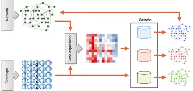
Therefore, to perform a rigorous comparison of the performance of different MCMC samplers and to investigate the conditions under which one sampler performs better than another, we designed a multifactorial simulation study with crossed factors. In our simulation study, network parameters played the role of factors, and the difference in area under the response curve of different samplers played the role of the response variable (Figure 1). By comparing the performance of methods across many different situations, the differences in performance we observe are less likely to be due to a specific parameter setting. Moreover, we can track how different types of network topology influence the performance of all methods or a specific method. This enables biologists to understand how
data sets with different origins and features are likely to affect the accuracy of estimated networks and which methods are optimized for the characteristics of a particular biological data set.
In our simulations, we investigated the effects of eight distinct simulation parameters, namely sample size, network topology, the number of network nodes, incorporation of genetic information, average edge density, average gene-to-gene signal, average SNP-to-gene-to-gene signal, and intrinsic expres-sion noise. (SeeMethodsfor further details.) These simulation variables were chosen to represent aspects of biological data sets that are reasonably expected to vary in a wide range of future applications. For instance, the strength of gene–gene correlations is controlled by a variety of biophysical processes such as transcription factor binding, chromosome configura-tion, and epigenetics (Gaiteri et al.2014). We compared the performance of four published MCMC samplers andfive novel sampler variations that we developed. The published samplers included (i) the foundational Metropolis–Hastings structure sampler (“STR sampler”) (Madigan et al. 1995; Giudici and Castelo 2003), (ii) the “REV” Metropolis–Hastings sampler (Grzegorczyk and Husmeier 2008), (iii) the single-parent set block Gibbs sampler (“1PB”), and (iv) the two-parent sets block Gibbs sampler (“2PB”) (Goudie and Mukherjee 2011). The new samplers included (v) the three-parent sets block Gibbs sampler (“3PB”), (vi) the four-parent sets block Gibbs sam-pler (“4PB”), (vii) the connected two-parent sets block sam-pler (“c2PB”), (viii) the connected three-parent sets block sampler (“c3PB”), and (ix) the connected four-parent sets block sampler (“c4PB”). Descriptions and comments on each of these samplers are provided in the Appendix.
Since our multifactorial design involves a large number of distinct factor-level combinations (1458 in total), and for each combination we run nine distinct MCMC samplers, we considered only a single replication per simulation param-eter combination. Each sampler was run for a fixed time with either a single longer chain or multiple shorter chains. Collectively, the experiment included 52,488 instances of reverse-engineering gene regulatory networks. To the best of our knowledge, this is the largest simulation study comparing MCMC samplers for structure learning in Bayesian networks.
Methods
Bayesian networks
Background and technical material on Bayesian networks and the MCMC samplers investigated in this study are pre-sented in theAppendix.
Setting of the MCMC runs
a chain and 20% of initial networks were discarded as burn-in. When running multiple chains, the chain length was controlled so that on average 50 chains completed in the time allotted. The last network of a chain was collected from each chain.
Program implementation
All the MCMC samplers were implemented in MATLAB 2012a (MathWorks). To conduct fair comparisons, the routines shared across the MCMC samplers were implemented in the same way by using the same subfunctions. Moreover, the routines specific for each MCMC sampler were highly opti-mized. All the programs were compiled by MATLAB Compiler to enable batch execution. The code to run all methods is available for download (DOI:10.7303/syn2910187).
Simulation parameters
The selection and range of simulation parameters were designed to reflect characteristics of typical systems genetics experiments. To investigate the relative performance of the different structure samplers, we designed a multifactorial simulation experiment with crossed factors, focusing on the effects of seven distinct simulation parameters, namely the following:
1. Network topology t, with levels “random” and “EIPO” (exponential in in-degree and power law on out-degree, as proposed by Guelzimet al.2002).
2. Number of network nodes,p, with levels“30,” “65,”and
“100.”
3. Edge density,d, with levels“low,” “medium,”and“high.” The edge density of a network is defined as the number of edges divided by the number of possible edges, namely, p3ðp21Þ: For each simulation, d was set to 0.02, 0.04, and 0.06 as low, medium, and high edge density, respectively. We did not limit the maximum num-ber of parent nodes in simulated networks, even though sampling methods often limit the number of possible parents, for reasons of computational efficiency.
4. Average gene-to-gene signal, h; defined as the average absolute value of the nonzero coefficients (of the regression of a gene on another). For each simulation,hwas sampled
uniformly from the ranges [0, 0.33], [0.33, 0.66], [0.66, 1] corresponding to low, medium, and high, respectively. 5. Intrinsic expression noise, s2; with levels low, medium,
and high, and defined as the variance of the error term, eNð0;s2Þ; used in the simulation of the expression
values (via linear structural equations). For each simula-tion,s2 was sampled uniformly from the ranges [0, 1],
[1, 2], [2, 3] corresponding to low, medium, and high, respectively.
6. Average SNP-to-gene signal, g; defined as the average absolute value of the nonzero coefficients (of the regres-sion of an expresregres-sion phenotype on a SNP). For each simulation, g was sampled uniformly from the ranges [0, 1], [1, 2], [2, 3] corresponding to low, medium, and high, respectively.
7. Sample size, n, with levels 100, 200, 300. This choice reflects typical sample sizes observed in the literature for causal gene networks (Zhanget al.2013).
In total, our experiment was conducted based on 2333 333333333 = 1458 distinct networks.
Simulation of network structures
We generated network structure based on EIPO topology observed in transcriptional regulatory networks (Guelzim et al. 2002). Random topology networks were also gener-ated as reference. We did not limit the maximum number of parent nodes for the simulated networks. Network struc-tures were generated using the SysGenSIM software (Pinna et al. 2011). This software allows the user to control the number of nodes and the network average degree (=2ðp21Þd), as well as choose among several topology types, including the random network topology and the EIPO topology. Although the software can also simulate genotype and expression data from experimental crosses (where the latter are generated according to nonlinear ordinary differ-ential equations), we do not employ those features for data generation. Instead, we generate genotype data from out-bred populations and simulate expression data from a mul-tivariate normal distribution consistent with the structural equation model representing the network structure.
Simulation of SNP data
To incorporate realistic genetics data in our simulations, we generate SNP data matrices by randomly selecting chunks of real SNP data from the HapMap3 database. To do this, we first randomly choosepgenes from the refGene in the UCSC Genome Browser and then select allcis-SNPs associated with thepgenes from genotype data on a Caucasian population. We define acis-SNP as any SNP physically located between (2) 110 kb upstream of the transcription start site and (+)40 kb downstream of the transcription end site, because this region is thought to contain 99% ofcis-eSNPs (e: expression single nu-cleotide polymorphism) (Veyrieraset al.2008).
Simulation of network data
Given the SNP data and a (possibly cyclic) directed network structure,G, with continuous (gene expression) and discrete (SNP) nodes, we generated multivariate normal gene ex-pression data with a covariance structure implied by the structural equation model (SEM) describing G. Because the SNP nodes are necessarily exogenous variables inG, the asso-ciated SEM can be represented, in matrix notation, as
X¼BXþCQþe (1)
(Liu et al.2008), where (i) eis ap3nmatrix of indepen-dent and iindepen-dentically distributed Nð0;s2Þ residual error
terms, (ii)Xis a p3nmatrix of expression levels, and (iii) Q is a k3n matrix of SNP genotype codes. B is a p3p matrix of gene-to-gene causal effects, where the element bijrepresents the partial regression coefficient of the
regres-sion of gene i on gene j. The structure of matrixB corre-sponds to the directed graph representing the interactions between the genes with edges corresponding of nonzero elements ofB. Because we adopt independent residual error terms, matrix B can be rearranged into a lower triangular matrix when G is acyclic, but will be necessarily nontrian-gular for cyclic graphs. C is a p3k matrix of SNP-to-gene causal effects. Each entry (i;j) of C represents the partial regression coefficient of the regression of geneion SNP j. The SNP-to-gene edges inGare represented by the nonzero elements ofC. Given the matricesB,C,Q, ande;we gener-ate the expression data matrix as X¼ ðI2BÞ21ðCQþeÞ: Note that because each column of e follows a Npð0;s2IpÞ
distribution, we have that the conditional distribution of each column Xj of X given B, C, and Q is
Np
ðI2BÞ21CQj;s2ðI2BÞ21ððI2BÞ21Þt
:Furthermore, no di-agonal dominance enforcement of ðI2BÞ was necessary to ensure matrix invertibility since the simulated networks were small; the diagonal and most of the off-diagonal entries ofB were zero (due to the absence of self loops and relatively low connectivity of the simulated networks), and the nonzero entries ofBconsisted of low values.
The values of the nonzero partial regression coefficients inB andCare sampled randomly from a uniform distribu-tion and then rescaled so that the average of their absolute values ishandg;respectively. The range of h;g;andr is
determined so that the variance of the expression phenotypes explained by eSNPs in simulated data covers that observed in real data, which ranges from 0.1 to 0.3 (Grundberget al.2012; McKenzie et al. 2014; Yang et al. 2014). In particular, the median variance explained by SNPs of our simulated data was 0.11 with a median absolute deviation of 0.15. An addi-tional constraint toCwas that 20% of the expression pheno-types have SNPs, which was based on the empirical proportion of genes with eSNPs, ranging from 5% to 35% (Brownet al. 2013). In addition, each such expression phenotype can have at most two SNPs, since three independent eSNPs for a single gene were very rare in studies with moderate sample size (Stranger et al.2012). Consequently, 80% of the rows of C are completely 0, and the remaining 20% of the rows can have at most two nonzero entries.
eSNP mapping
We perform eSNP mapping tailored to the network structure by evaluating conditional independence relations between expression traits and SNPs, given their expression trait parents (Chaibub Neto et al. 2010). The likelihood ratio between the full model and the null model that is generated by removing the SNPs term from the equation can be used as a formal test of conditional independence. The empirical null distribution of the likelihood ratio is estimated by 1000 permutations of individual labels as follows. At each time, the individual labels of either expression trait or SNPs were randomly permuted so that relations between expres-sion trait and SNPs were broken while keeping the correla-tion structure among expression traits intact (and while preserving the correlation structure of the SNPs as well). Then the likelihood ratios of all the pairwise relationships between expression traits and their cis-SNPs were calcu-lated, followed by the collection of the maximum value across all computed likelihood ratios. The permutation null distribution generated by this procedure is then used to test the null hypothesis of detecting an association given that none of the SNPs are associated with the expression trait. The genome-wide error rate of detecting cis-eSNP associa-tions was controlled at 0.05.
Performance measures
We evaluated network reconstruction performance, using the area under the curve of the precision-recall plot (AUCPR), where
precision ¼ number of true positives total number of edges detected;
recall ¼ number of true positives total number of true edges;
for performance evaluation. AUCROC is a composite mea-sure based on true positive rate (recall) and false positive rate, defined as
false positive rate ¼ number of false positives total number of true absent edges;
where a false positive was defined as an inferred directed edge that did not exist in the true network used to generate the expression data.
Results
Network characteristics affect the performance of Bayesian network reconstruction
To elucidate effects of various biological characteristics on network estimation accuracy, we performed a systematic sim-ulation experiment with an ensemble of systems genetics data where each parameter (network characteristic) was sampled over a biologically plausible range. To evaluate the accuracy of an estimated network, we applied Bayesian model averaging to the probabilistic network estimates produced by any given method, to obtain a composite adjacency matrix. Then, AUCPR as adopted as a measure of correctness of an output adjacency matrix, given a true network. Using this response variable, we used ANOVA to identify network features that have significant impact on the performance of network reconstruction.
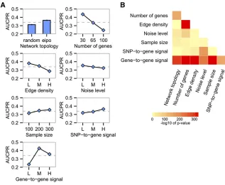
All the network characteristics tested, as well as various 232 interactions among these, were found to be significantly associated with AUCPR (Figure 2), but the strength of the effects and form of the interactions varied widely. Our exper-iment indicates that network topology affects the accuracy of network reconstruction. Networks with EIPO topology were reconstructed more accurately than those with random topol-ogy (Figure 2A). The experiment also identified harmful and beneficial effects of network characteristics on estimation ac-curacy. The increase in the number of genes, edge density, and noise level decreased AUCPR monotonically. Conversely, the increase of sample size and strength of SNP-to-gene signal positively contributed to the accuracy of reverse engineering (Figure 2A). Unlike the other network characteristics, gene-to-gene signal strength showed a nonmonotonic effect on AUCPR (Figure 2A). Initially, the increase in gene-to-gene signal strength had a beneficial effect on performance because stron-ger signals aided in distinguishing true regulations from noise. However, once the gene-to-gene signal strength exceeded a cer-tain point, it showed the opposite effect (Figure 2A). Strength of gene-to-gene signal also showed significant interactions with other characteristics, including sample size, the number of genes, edge density, and network topology (Figure 2B). How-ever, these interactions did not alter the nonmonotonic trend of the effect of gene-to-gene signal on AUCPR (Supporting Information,Figure S1).
We found that secondary effects of gene-to-gene signaling accounted for the nonmonotonic effect of gene-to-gene signal on AUCPR. We observed that high average gene-to-gene signal
strength monotonically increased the correlations between directly connected genes and also those between indirectly connected genes (Figure 3A). These indirect effects of gene-to-gene signal strength were quantified byM= log10(directCor/ indirectCor) based on the average correlations of directly con-nected genes and those of indirectly concon-nected genes. ThisM measure showed a nonmonotonic trend along with the amount of gene-to-gene signal strength (Figure 3A) and was well cor-related with AUCPR (Figure 3B). This suggests that the poor network reconstruction performance against networks with high gene-to-gene signal is due to the low Mof the data set through the increase of indirect signals.
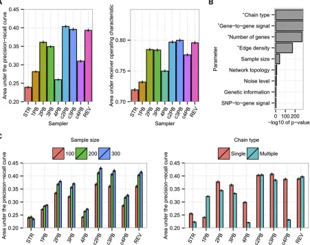
Comparison of structural samplers
Next we investigated general performances of structural samplers. For rigorous quantification, both AUCPR and AUCROC were employed as performance measures. Based on these measures, c2PB, c3PB, and REV outperformed other samplers, whereas STR, a traditional sampler, showed the worst perfor-mance (Figure 4A). The main methodological difference be-tween top-performing samplers c2PB, c3PB, and REV and STR is the magnitude of modifications to a network offered at each step. Specifically, REV and c2PB update parents of two nodes and c3PB updates parents of three nodes simultaneously at each step. By contrast, STR modifies only a single edge of a network at each step. Superior performance of c2PB, c3PB, and REV was quite robust over many types of networks tested (Figure S2), suggesting samplers that execute drastic network modifications at a single step can potentially generate more accurate network structures within a set time compared to methods that employ smaller updates.
information criterion (BIC) of multiple chains is higher than that of a single chain (Figure S3), which resulted in lower AUCPRs. Conversely, the samplers including 1PB, c2PB, and REV that reach a stationary distribution faster would have potential ben-efits from exploring optimal networks over the large network space by employing shorter multiple chains from different initial networks. We note, however, that the minimum BIC of each sampler did not depend on the convergence speed (Figure S3). This suggests that some samplers with fast convergence speed such as 1PB can reach suboptimal networks quickly, but are not able to exit from the suboptimal configuration state.
To classify MCMC samplers based on their performance, we used hierarchical clustering analysis of AUCPR and AUCROC results (Figure 5). In this analysis, we treated a sin-gle longer chain and multiple shorter chains as separate methods. The clustering analysis based on the AUCPR result suggested MCMC samplers can be clustered into four types, which were driven by differences in performance on four primary types of data sets (Figure 5). Examination of net-work characteristics associated with the four groups of data sets revealed the number of genes, edge density, and gene-to-gene signal strength are major characteristics that differ-entiate the performance of various samplers (Figure S4A). In AUCPR-based clustering, 1PB, 2PB, and 3PB running with multiple shorter chains were in the same group and showed strong performance, especially for networks with high num-bers of genes, high edge density, and high gene-to-gene signal strength. The top-performing samplers, c2PB, c3PB, and REV, were also clustered together and worked well across many simulations, except for networks with low gene-to-gene signals. STR and 4PB fell into the same cluster, showing poor performances over most network results. In the AUCROC-based clustering, we also observed four clusters of
MCMC samplers and four groups of datasets (Figure 5). The three network characteristics, numbers of genes, edge density, and gene-to-gene signal strength were again associated with the four groups of data sets (Figure S4B). This further sup-ports the large impact of these three network parameters on the accuracy of the reverse engineering of gene-regulatory networks. Similar to the AUCPR result above, 1PB, 2PB, and 3PB and c2PB, c3PB, and REV clustered into the same group (Figure 5). However, the strongest factor contributing to the cluster separation was the chain type employed. Run-ning with multiple chains resulted in clearly higher AUCROC than with single-chain execution.
Detailed comparison of top-performing samplers
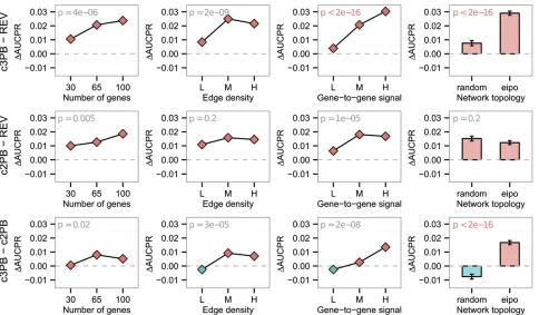
Next we investigated the differences among the top-performing samplers, REV, c2PB, and c3PB. To evaluate rel-ative performance of any pair of structure samplers,AandB, we used single-replicate multiway ANOVA, with the response given byWAB= AUCPRA –AUCPRB. We focus here on the
signal and network topology, are associated with the difference between c3PB and c2PB, just as they are between c3PB and REV (Figure 6). These results demonstrate that a newly de-signed sampler, c3PB, is superior to REV, especially for highly correlated biological networks.
Evaluation of the effect of genetic information
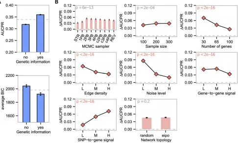
We designed our algorithm to incorporate SNPs as nodes in a Bayesian network, which means we estimated the struc-ture of gene-to-gene networks and the eSNP mapping simultaneously. The incorporation of SNPs creates new sets of conditional independence relations, allowing us to distin-guish between gene regulatory networks with equivalent likelihood. Furthermore, by including SNPs in the model we can potentially improve the model fit, leading to higher network recovery scores. We evaluated the benefit of in-corporating SNP information for both the accuracy of the estimated network and the modelfit to gene expression data, as follows. First, gene expression data and SNP data were simulated from networks composed of genes and SNPs. Then, gene expression data alone or both gene expression and SNPs were applied to the Bayesian network estimation programs.
Our results show that AUCPR and average BIC score significantly improve when both gene expression data and SNP data are used for reverse engineering (Figure 7A). We also investigated parameters that affected the performance gain when SNPs were incorporated (Figure 7B). As the strength of SNP-to-gene signal ramped up, the benefit of in-corporating SNPs also increased the network reconstruction accuracy. Conversely, as the number of genes, edge density, and noise level increased, the beneficial effect of SNPs became more limited. The effects on inferred network accuracy that stem from incorporating SNPs are independent of MCMC sam-pler, sample size, and network topology. Our simulation study indicates that SNP information is often helpful to estimate Bayesian networks, but might be less effective on data sets generated by real networks that are large, are noisy, or have dense sets of interactions.
Discussion
Reverse engineering of gene networks from systems genetics data (Jansen 2001) is an active research area. Although we focused on MCMC samplers for gene network structure learn-ing in the present article, many other statistical approaches/ frameworks have been proposed in the literature. For instance, Chaibub Netoet al.(2008) applied the PC algorithm (Spirtes et al. 2000) to first infer the skeleton of the gene network and then used expression QTL (eQTL) to determine the direc-tions of the edges in the phenotype network. Liuet al.(2008) proposed a two-step approach wherein an encompassing directed network (EDN) is first generated from assembled pairwise regulator–target relationships (which might be direct or indirect), followed by the application of structural equation models to search for a (possibly) cyclic network nested in the EDN, which bestfits the data according to the BIC criteria. By restricting the network space to networks nested in the EDN, this approach is able to handle networks with hundreds of genes and eQTL. Logsdon and Mezey (2010) proposed a multiple-step approach where an association analysis is carried out to identify local eQTL, followed by the inference of an un-directed network of gene expression traits and eQTL nodes via a covariance selection approach based on the adaptive lasso feature selection procedure and subsequent mapping of the un-directed network into a possibly cyclic gene expression network. Zhang and Kim (2014) adopted sparse conditional Gaussian graphical models for modeling undirected gene networks under SNP perturbations, where the gene network structure learning task and the SNP feature selection task are performed jointly by solving a single optimization problem containing the lasso (for SNP feature selection) and the graphical lasso (for gene net-work structure learning) as special cases.
A common feature of these non-Bayesian approaches is that the output of the reverse-engineering algorithm is a single point estimate of the gene network, and no statistical measure of uncertainty about the inferred network is available. The MCMC samplers, on the other hand, output an entire poste-rior distribution of network structures, from which Bayesian Figure 3 Tracking both direct and indirect gene-to-gene correlations explains how moderate correla-tions lead to the most accurate network inference. (A) Increasing the gene-to-gene signal strength increases the average correlation between genes, as expected. The strength of indirect correlations be-tween genes also increases as gene-to-gene signal strength increases. Direct and indirect correlations are the average correlation of directly connected genes and indirectly connected genes, respectively. TheMmeasure represents the log10 ratio between direct correlation and indirect correlation in each data set. (B) The bell-shaped response of AUCPR to increasing direct gene-to-gene correlations might be unexpected, but once the concurrent increase of in-direct correlations is taken into account (through the
model-averaged estimates of the probability for the presence and direction of any particular edge in the network are readily available. This provides information about which parts of the inferred network were reconstructed with stronger confidence. This feature is particularly important for reverse engineering of gene networks since expression data are notoriously noisy. The main drawback is the increased computational requirements, compared to non-Bayesian/point estimate approaches, which are generally faster and scalable to larger networks. Nonetheless, MCMC approaches have been successfully applied to genome-scale real data (Zhuet al.2008; Zhanget al.2013) byfirst clustering the gene expression data into much smaller groups via weighted gene coexpression analysis (Zhang and Horvath 2005), followed by Bayesian networks reconstruction for the separate and more manageable gene clusters.
MCMC samplers based on moves in the space of node orders (Friedman and Koller 2003; Eaton and Murphy 2007; Ellis and Wong 2008) have been shown to considerably im-prove the mixing of the Markov chain. Nonetheless, these sam-plers do not allow the explicit specification of prior distributions over network structures. Since our main applied interest is the
reconstruction of Bayesian networks with noisy genomic data, where the incorporation of prior knowledge can improve re-construction performance, we focus our attention on MCMC approaches based on moves in network structure space.
To investigate network inference in the context of data sets that are likely encountered by experimental biologists, we conducted the largest simulation study comparing MCMC samplers for structure learning in Bayesian networks to date. By ranging over combinations of biologically plausible param-eter settings, we can be confident in our conclusions about the relative performance of different inference methods. The variability in generative network structures also allows us to understand how network characteristics affect the performance of various network inference methods. Specifically, our simu-lation study is designed in the spirit of a multifactorial ex-periment with crossed factors, where simulation parameters play the role of factors. This allows us to investigate the effect of each parameter on the accuracy of Bayesian networks, in addition to comparing performance of MCMC samplers.
average edge density increased, the learning performance of every method decreased monotonically. One possible reason for this behavior is that for Bayesian network inference, we restricted the number of parents to,= 3, to reduce the size of the network space to evaluate. On the other hand, we did not pose any restriction on the number of parents in simu-lated networks where the maximum edge density was set as 0.06, which means each node in networks with size 30, 65, and 100, is expected to have 1.8, 3.9, and 6 parents on average, respectively, assuming random network topology. Because of this limitation, it is possible that we miss some true incoming regulatory relationships for genes that are regulated by many other genes. However, in real applica-tions, since screening the genes with many children is likely to be a predominant question of interest, this limitation may not be critical. Another reason for the generally harmful effect of edge density on performance could be the correla-tion strength of the data set. In our simulacorrela-tion framework, the average gene-to-gene correlation is influenced by edge density and the strength of gene-to-gene signaling. Gener-ally, it is difficult to estimate true regulations in a highly correlated data set, since the Markov equivalence classes of a directed network cannot be identified uniquely (Uhler et al. 2013). STR, the simplest sampler, showed the worst performance against networks with high edge density and high gene-to-gene signal, probably due to being trapped in suboptimal structures. This limitation has practical consequen-ces for recent attempts to define causal networks within gene coexpression networks, since those coexpression networks are composed of correlated gene variables. However, our
new sampler, c3PB, showed better performance compared with STR as well as REV, for the networks with high gene-to-gene signal, indicating c3PB works well for elucidating complex and correlated biological networks.
factors such as the strength of the SNP-to-gene associations also contribute to the total percentage of variance explained by SNPs in real systems. While wefix the number of genes with eSNPs, we still examine a range of scenarios for percentage of variance explained by SNPs, because we utilize three levels of SNP-to-gene coupling.
Zhuet al.(2007) provided a detailed simulation investiga-tion of the effect of the integrainvestiga-tion of genetic and expression data in Bayesian network reconstruction performance. They focused on simulations from a single (biologically motivated) network structure, in contrast to our present study investigat-ing many characteristics across 1458 distinct and biologically plausible networks. In Zhuet al.(2007), the authors concluded that the integration of SNP and expression data can greatly improve network reconstruction. In our simulations, we also observed that the genetic information has beneficial effects, but found that the effect size for genetics is smaller than the effect of other parameters, such as the particular method employed. We further clarified the benefit of genetics by show-ing that the advantage of includshow-ing genetics was maximized when the strength of SNP-to-gene signal was high and the intrinsic noise was low. Signal strength and noise level actually determine the extent of SNPs’contribution to gene expression levels. The middle range of signal strength and noise level corresponds to an average effect size of eSNPs commonly observed in real data. At this level of effect size, improper selection of an inference method and running setting of the MCMC chain potentially diminishes the benefit of utilizing
SNP information. Alternatively, for systems where SNPs strongly influence expression, incorporating SNP data can pro-duce a greater marginal increase in performance than the choice of MCMC method. For instance, incorporation of SNP data will likely be most beneficial for causal network inference of gene expression phenotypes clustered in strong hotspots.
1PB, the performance of 4PB decreased substantially (Figure 4A). Although the use of higher-order parent blocks improves the mixing of the Markov chain, it also exponentially increases the amount of computation necessary to keep track of the allowable combinations of parent sets, so that the number of steps completed by the sampler in afixed time window is de-creased. Hence, in spite of the better mixing of the chain, we still observe a performance drop. These results indicate that both drastic modifications for escape from suboptimal net-works and computational efficiency are important in effective sampler operation.
We designed“connected”block Gibbs methods, as a hy-brid of the classic block Gibbs and REV methods, motivated by limitations of the older methods exposed by our simulation framework. At a given time step, both REV and 2PB update the parent sets of two nodes. However, the performance of 2PB was inferior to that of REV (Figure 4A). This result was un-expected because Gibbs samplers accept network modification at every step and thus are potentially more efficient than a Metropolis–Hastings sampler. A major difference between 2PB and REV that accounts for this is that 2PB updates parent sets of every pair of two nodes sequentially, whereas REV updates only parent sets of the two connected nodes. Therefore, we designed c2PB, which performs 2PB updates for only the two connected nodes at each step and also extended c2PB to ones
with higher-order blocking, namely c3PB and c4PB. Figure 4A shows our connected PB samplers clearly improve the formal PB Gibbs samplers, resulting in comparable or better perfor-mance than that of REV. The perforperfor-mance improvements of cPB likely result from two sources. First, the speed of chain convergence is higher in cPBs compared with corresponding PBs (Figure S3). Second, cPBs can reach networks with lower BIC, meaning optimized network structures explain the data set better (Figure S3). These improvements are also evident when comparing c2PB with REV. cPBs can be seen as weighted versions of a PB sampler. Specifically, each gene is not updated with equal frequency, but rather the update probability for each gene is weighted based on the current network structure. Since cPBs weight all linearly connected gene pairs uniformly, a more complex weighting procedure may be useful to explore in the future.
the enormous space of possible networks, which is superexpo-nential with the number of nodes. For instance, networks from our “medium-size” simulations containing 65 nodes have a number of possible configurations that exceed the estimated number of atoms in the observable universe. Both algorithmic advances in network update steps or brute-force computational approaches could be used to improve network inference, with more efficient or more comprehensive approaches to exploring this huge search space. Our method comparison primarily fo-cuses on algorithmic advances, although computational con-straints also influenced the results, especially for inefficient methods. From a computational perspective, starting from many different random networks can help to avoid becoming stuck in local minima, as can performing more drastic update moves. Our results for singlevs.multiple chains indicate that 1PB, c2PB, c3PB, and REV methods that converge rapidly will benefit the most from a massively parallel approach tofinding optimal networks. But results from the classic STR method demonstrate that even an excess of computational resources is not sufficient to overcome a method that is easily trapped in local optima. At the same time, limitations on computational capabilities can hold back algorithms that should produce su-perior performance. For instance, we see increasing perfor-mance across 1PB, 2PB, and 3PB, yet perforperfor-mance of 4PB falls off, as computational overhead overcomes its theoretical advantages. Therefore, based on this simulation study, our general advice for future applications of the methods tested here is to devote substantial computational resources to the latest methods, such as c3PB, that are able to benefit from these resources. If a data set is known to have particular char-acteristics such as high levels of noise, etc., then the recom-mended method will shift to one that is known to function well under that regime, although we note that some methods such as c3PB function well under a majority of tested scenarios.
One practical goal of network inference methods in early-stage drug discovery is to identify a small number of genes that control a specific molecular network or a disease signature. Perturbation experiments in model disease systems indicate that causal networks can indeed predict some disease-relevant genes and downstream targets (Chen et al.2008; Yang et al. 2009). While large-scale causal network inference has been most frequently applied to data from mouse crosses whose common genetic background creates strong eQTL, these meth-ods have also been applied to paired genetics and gene expres-sion data sets from humans (Zhanget al.2013). However, these previous applications employed variants of the STR method, which is outperformed by all other methods tested here. While previous studies have made some correct predictions, there are also numerous false positive and false negative predictions, based on comparing the expectedvs.actual (measured) down-stream targets of perturbed genes in model systems (Zhang et al. 2013). The greater accuracy of top-performing methods is therefore key to deriving accurate predictions from human expression data sets, with or without genetics.
Because many gene expression studies do not include paired genetics data, correlation-based coexpression networks
are frequently used to attempt to identify key disease genes (Gaiteri et al. 2014). Specifically, hub genes within disease-correlated networks are often invoked as key disease genes. However, coexpression hubs are not necessarily causal in gen-erating a phenotype of gene signature, because a gene at the top of a regulatory cascade may have only a few direct inter-actions. Such genes may be ignored when focusing on coex-pression hub genes. Similarly, hub genes may be subject to incoming regulatory relationships, which cannot be detected in an undirected coexpression framework. Our simulations show that for typical human data sets, even in the absence of genetic priors, we can identify conditional dependence net-works of genes that accurately reflect the true regulatory struc-ture. This sparse hierarchical output could be utilized to aid in selecting genes that control a particular disease-relevant mo-lecular system. Causal networks could even be useful in de-fining relationships across different diseases, to find directed interactions that mediate comorbidity. However, such data sets likely involve .100 genes, which entails a large network search space. The potential of causal inference to identify hu-man regulatory networks among a large number of genes, with or without genetic priors, reinforces the need to use top-performing methods that do not become trapped in suboptimal/ inaccurate network states.
Literature Cited
Aten, J. E., T. F. Fuller, A. J. Lusis, and S. Horvath, 2008 Using genetic markers to orient the edges in quantitative trait net-works: the NEO software. BMC Syst. Biol. 2: 34.
Beinlinch, I., H. Suermondt, R. Chavez, and G. Cooper, 1989 The ALARM monitoring system: a case study with two probabilistic inference techniques for belief networks, pp. 247–256 inIn Second European Conference on Artificial Intelligence in Medicine, edited by J. Hunter, J. Cookson, and J. Wyatt. Springer-Verlag, Berlin. Brown, C. D., L. M. Mangravite, and B. E. Engelhardt,
2013 Integrative modeling of eQTLs and cis-regulatory ele-ments suggests mechanisms underlying cell type specificity of eQTLs. PLoS Genet. 9: e1003649.
Chaibub Neto, E., C. T. Ferrara, A. D. Attie, and B. S. Yandell, 2008 Inferring causal phenotype networks from segregating populations. Genetics 179: 1089–1100.
Chaibub Neto, E., M. P. Keller, A. D. Attie, and B. S. Yandell, 2010 Causal graphical models in systems genetics: a unified framework for joint inference of causal network and genetic architecture for correlated phenotypes. Ann. Appl. Stat. 4: 320–339.
Chaibub Neto, E., A. T. Broman, M. P. Keller, A. D. Attie, B. Zhang et al., 2013 Modeling causality for pairs of phenotypes in sys-tem genetics. Genetics 193: 1003–1013.
Chen, L. S., F. Emmert-Streib, and J. D. Storey, 2007 Harnessing naturally randomized transcription to infer regulatory relation-ships among genes. Genome Biol. 8: R219.
Chen, Y., J. Zhu, P. Y. Lum, X. Yang, S. Pinto et al., 2008 Variations in DNA elucidate molecular networks that cause disease. Nature 452: 429–435.
Duarte, C. W., and Z.-B. Zeng, 2011 High-confidence discovery of genetic network regulators in expression quantitative trait loci data. Genetics 187: 955–964.
Annual Conference on Uncertainty in Artificial Intelligence (UAI-07), Corvallis, OR, pp. 101–108.
Ellis, B., and W. H. Wong, 2008 Learning causal Bayesian net-work structures from experimental data. J. Am. Stat. Assoc. 103: 778–789.
Ferrara, C. T., P. Wang, E. Chaibub Neto, R. D. Stevens, and J. R. Bain et al., 2008 Genetic networks of liver metabolism re-vealed by integration of metabolic and transcriptional profiling. PLoS Genet. 4: e1000034.
Friedman, N., and D. Koller, 2003 Being Bayesian about network structure. Mach. Learn. 50: 95–126.
Gaiteri, C., Y. Ding, B. French, G. C. Tseng, and E. Sibille, 2014 Beyond modules and hubs: the potential of gene coex-pression networks for investigating molecular mechanisms of complex brain disorders. Genes Brain Behav. 13: 13–24. Giudici, P., and R. Castelo, 2003 Improving Markov chain Monte
Carlo model search for data mining. Mach. Learn. 50: 127–158. Goudie, R. J. B., and S. Mukherjee, 2011 An efficient Gibbs sam-pler for structural inference in Bayesian networks. Paper no. 11-21. Center for Research in Statistical Methodology. Coventry, United Kingdom. Available at:www.warwick.ac.uk/go/crism. Grundberg, E., K. S. Small, A. K. Hedman, A. C. Nica, A. Builet al.,
2012 Mapping cis- and trans-regulatory effects across multiple tissues in twins. Nat. Genet. 44: 1084–1089.
Grzegorczyk, M., and D. Husmeier, 2008 Improving the structure MCMC sampler for Bayesian networks by introducing a new edge reversal move. Mach. Learn. 71: 265–305.
Guelzim, N., S. Bottani, P. Bourgine, and F. Képès, 2002 To-pological and causal structure of the yeast transcriptional regu-latory network. Nat. Genet. 31: 60–63.
Hageman, R. S., M. S. Leduc, R. Korstanje, and B. Paigen, and G. A. Churchill, 2011 A Bayesian framework for inference of the genotype-phenotype map for segregating populations. Genetics 187: 1163–1170.
Huang, T. L., P. P. Zandi, K. L. Tucker, A. L. Fitzpatrick, L. H. Kuller et al., 2005 Benefits of fattyfish on dementia risk are stronger for those without APOE epsilon4. Neurology 65: 1409–1414. Jansen, R., 2001 Genetical genomics: the added value from
seg-regation. Trends Genet. 17: 388–391.
Kass, R. E., and AE. Raftery, 1995 Bayes factors. J. Am. Stat. Assoc. 90: 773–795.
King, V., and G. Sagert, 2002 A fully dynamic algorithm for main-taining the transitive closure. J. Comput. Syst. Sci. 65: 150–167. Liu, B., A. de la Fuente, and I. Hoeschele, 2008 Gene network inference via structural equation modeling in genetical ge-nomics experiments. Genetics 178: 1763–1776.
Liu, M., A. Liberzon, S. W. Kong, W. R. Lai, P. J. Park et al., 2007 Network-based analysis of affected biological processes in type 2 diabetes models. PLoS Genet. 3: e96.
Logsdon, B. A., and J. Mezey, 2010 Gene expression network re-construction by convex feature selection when incorporating genetic perturbations. PLoS Comput. Biol. 6: e1001014. Madigan, D., J. York, and D. Allard, 1995 Bayesian graphical
models for discrete data. Int. Stat. Rev. 63: 215.
McKenzie, M., A. K. Henders, A. Caracella, N. R. Wray, and J. E. Powell, 2014 Overlap of expression quantitative trait loci (eQTL) in human brain and blood. BMC Med. Genomics 7: 31. Moon, J. Y., E. Chaibub Neto, B. S. Yandell, and X. Deng, 2014 Bayesian causal phenotype network incorporating genetic variation and biological knowledge, pp.165–195 in,Probabilistic Graphical Models in Genetics,Genomics,and Postgenomics, edited
by C. Sinoquet, and R. Mourad. Oxford University Press, Lon-don/New York/Oxford.
Pearl, J., 1988 Probabilistic Inference in Intelligent Systems. Mor-gan Kaufmann, San Mateo, CA.
Peila, R., B. L. Rodriguez, and L. J. Launer, 2002 Type 2 diabetes, APOE gene, and the risk for dementia and related pathologies: The Honolulu-Asia Aging Study. Diabetes 51: 1256–1262. Pinna, A., N. Soranzo, I. Hoeschele, and A. de la Fuente,
2011 Simulating systems genetics data with SysGenSIM. Bio-informatics 27: 2459–2462.
Rhinn, H., R. Fujita, L. Qiang, R. Cheng, J. H. Lee et al., 2013 Integrative genomics identifies APOEe4 effectors in Alz-heimer’s disease. Nature 500: 45–50.
Schadt, E. E., J. Lamb, X. Yang, J. Zhu, S. Edwardset al., 2005 An integrative genomics approach to infer causal associations be-tween gene expression and disease. Nat. Genet. 37: 710–717. Spirtes, P., C. Glymour, and R. Scheines, 2000 Causation,
Predic-tion,and Search. MIT Press Cambridge, MA
Stegle, O., L. Parts, R. Durbin, and J. Winn, 2010 A Bayesian framework to account for complex non-genetic factors in gene expression levels greatly increases power in eQTL studies. PLoS Comput. Biol. 6: e1000770.
Stranger, B. E., S. B. Montgomery, A. S. Dimas, L. Parts, O. Stegle et al., 2012 Patterns of cis regulatory variation in diverse hu-man populations. PLoS Genet. 8: e1002639.
Uhler, C., G. Raskutti, P. Bühlmann, and B. Yu, 2013 Geometry of the faithfulness assumption in causal inference. Ann. Stat. 41: 436–463.
Veyrieras, J.-B., S. Kudaravalli, S. Y. Kim, E. T. Dermitzakis, Y. Gilad et al., 2008 High-resolution mapping of expression-QTLs yields insight into human gene regulation. PLoS Genet. 4: e1000214.
Wagner, G. P., and J. Zhang, 2011 The pleiotropic structure of the genotype-phenotype map: the evolvability of complex organ-isms. Nat. Rev. Genet. 12: 204–213.
Yang, S., Y. Liu, N. Jiang, J. Chen, L. Leachet al., 2014 Genome-wide eQTLs and heritability for gene expression traits in unre-lated individuals. BMC Genomics 15: 13.
Yang, X., J. L. Deignan, H. Qi, J. Zhu, S. Qianet al., 2009 Validation of candidate causal genes for obesity that affect shared metabolic pathways and networks. Nat. Genet. 41: 415–423.
Zhang, B., and S. Horvath, 2005 A general framework for weighted gene co-expression network analysis. Stat. Appl. Genet. Mol. Biol. 4: 1–45.
Zhang, B., C. Gaiteri, L.-G. Bodea, Z. Wang, J. McElwee et al., 2013 Integrated systems approach identifies genetic nodes and networks in late-onset Alzheimer’s disease. Cell 153: 707– 720.
Zhang, L., and S. Kim, 2014 Learning gene networks under SNP perturbations using eQTL datasets. PLoS Comput. Biol. 10: e1003420.
Zhu, J., M. C. Wiener, C. Zhang, A. Fridman, E. Minch et al., 2007 Increasing the power to detect causal associations by combining genotypic and expression data in segregating popu-lations. PLoS Comput. Biol. 3: e69.
Zhu, J., B. Zhang, E. N. Smith, B. Drees, R. B. Brem et al., 2008 Integrating large-scale functional genomic data to dis-sect the complexity of yeast regulatory networks. Nat. Genet. 40: 854–861.
Appendix
Bayesian Networks Background and Notation
A Bayesian network (Pearl 1988) is a multivariate probabilistic model whose conditional independence relations can be represented graphically by a directed acyclic graph (DAG) withvertices V¼ ðV1; :::;VpÞanddirected edgesði; jÞ 2E⊂V3V
(note that we use the notationsiandViinterchangeably, to refer to a node). Ifði;jÞ 2E;we sayiis aparentofjandjis achild
ofi. We define adirected pathas any unbroken, nonintersecting sequence of vertices in a graph that go along the direction of the edges. We say that a descendant of a vertex iis any vertex jsuch that there is a directed path from ito j, whereas anondescendantofiis any vertexk such that there is no directed path fromitok. A vertex jin a DAG Gcorresponds to a random variableXjin the Bayesian network. Assuming the local directed Markov property that states that each variable is
independent of its nondescendant variables conditional on its parent variables, we can factor the joint distribution as
PðXjGÞ ¼Y p
j¼1
PðXjjXGjÞ; (A1)
whereX¼ ðX1; :::;XpÞT;Gjis the set of parents ofj, andXGj ¼ fXi:i2Gjg. Note thatGcan be decomposed into a set of parent
sets such thatG¼ ðG1; :::;GpÞ ¼ ðGj;G2jÞ;whereG2j¼ ðG1; :::;Gj21;Gjþ1; :::;GpÞ;and that the prior predictive distribution in
(A1) factorizes across vertices into local components PðXjjXGjÞthat are functions of these parent sets. The network scores are
computed according to the BIC approximation to the prior predictive distribution (Kass and Raftery 1995). For structure learning, we focus on the posterior distribution of DAG structures
PðGjXÞ ¼PPðXjGÞPðGÞ
G2GPðXjGÞPðGÞ
; (A2)
wherePðGÞis a prior on the network structureG, andGrepresents the space of all DAGs withpvertices. This posterior is the target equilibrium distribution for the MCMC samplers described in the next section.
Checking for Cycles
The main computational cost for structure samplers is due to checking for cycles. Following Goudie and Mukherjee (2011), we adopt the algorithm from King and Sagert (2002), for cycle checking, in our implementations. This algorithm tracks the transitive closure of the current state of the sampler, represented by matrixTG;which, for a graphG, is represented as the
directed graphðV;E*Þ;where ðVi;VjÞ 2E* if and only if a path exists fromVito Vj:Inspection of the adjacency matrix of
the transitive closure shows which network modifications can be made without introducing a cycle in the following way: the addition of an edgeði;jÞwill introduce a cycle if and only ifTG
ji ¼1;whereas the removal of an edge can never introduce
a cycle. An efficient implementation of this algorithm keeps track of a path count matrixCG(with rows indexing parents,
columns indexing children, off-diagonal entries representing the number of distinct paths fromVitoVjinG, and diagonal
entries set to 1). Observe thatTG
ij ¼1 if and only if CijG.0; and query operations can be performed by simply checking
whether the relevent entries are positive. As pointed by Goudie and Mukherjee (2011), updating CG is straightforward.
Consider a graphG9formed by adding an edgeði;jÞto graphG. LetCG
i represent theith column ofC
GandCG
jrepresent thejth row ofCG:Then the updated count matrix for the addition of an edgeði;jÞis computed asCG9¼CGþCG
i5C G
j;whereas the
updated count matrix after the deletion of an edgeði;jÞis computed asCG9¼CG2CG
i5C G j:
Summary Characteristics of Structure MCMC Samplers for Learning Bayesian Networks
The STR sampler (Madigan et al. 1995; Giudici and Castelo 2003)
The STR sampler performs simple modifications to the current DAG state. At each iteration, it adds, drops, or reverses a single edge of the network and accepts the modified network according to the standard Metropolis–Hastings acceptance probability. Each time an edge is added or reversed, it is necessary to check whether the new network has a cycle, and if it does, the move needs to be discarded. [This sampler was proposed by Giudici and Castelo 2003 as an improvement over the Markov chain Monte Carlo model composition (MC3) sampler proposed by Madiganet al.1995 that considered only addition
The REV sampler (Grzegorczyk and Husmeier 2008)
The REV sampler adopts an alternative edge reversal move (“REV move”) to improve the mixing of the Markov chain. The steps to perform this network alteration are (i) select an edge whose direction is to be reversed; (ii) for each of the nodes connected by the selected edge, drop the incoming edges (that is, “orphan” the nodes); (iii) reverse the direction of the selected edge; and (iv) sample new parents for the nodes involved in the edge reversal (in addition to keeping the reversed edge) with a probability proportional to their scores. Note that contrary to the STR sampler, which allows the reversal of an edge only if it leads to a new valid DAG, the REV move always leads to a DAG. Even for those edges that could be reversed by the STR reversal move, it is still advantageous to use the REV move since it usually leads to higher acceptance rates. It does this by sampling completely new parent sets, instead of simply changing the direction of a single edge. Because the adoption of the REV move alone does not guarantee the ergodicity of the Markov chain, the REV sampler is actually implemented as a combination of REV and STR moves. In this article we adopt a sampler with REV moves performed in 50% of the iterations.
The single-parent set block Gibbs sampler—1PB (Goudie and Mukherjee 2011)
Because our novel samplers are extensions of the block Gibbs samplers proposed by Goudie and Mukherjee (2011), we present their method in greater detail in this section and the next section. For Bayesian networks the most natural blocks are given by the parent sets of each node. Because the prior predictive distribution factorizes according to each node and its parent set, we can parameterize a DAGGaccording to the parent setsGjof each vertexj¼1; :::;p;such that the posterior
distribution ofGis represented by
PðG1;. . .;GpjXÞ}P
G1;. . .;Gp
Yp
j¼1
PðXjjXGjÞ: (A3)
To construct a block Gibbs sampler over the parent set blocks, we need to construct the full conditional distributions of each parent set, conditional on all other parent sets. Because Bayesian networks are DAGs, we have that parent setsGj;for
whichG¼ ðGj;G2jÞ is cyclic, must have probability zero, and the full conditional distribution ofGjgivenG2jis given by
PðGjjG2j;XÞ ¼
PðGj;G2jjXÞ
P
Gj2K*j
PðGj;G2jXÞ
; (A4)
whereK*
j represent the set of parent setsGjsuch thatGis acyclic. The computation ofKj*can be done efficiently, using the
path count matrix. Recall that adding an edgeði;jÞwill introduce a cycle if and only ifCG
ji.0:Therefore, the set of nodes that
can be added as parents ofVjis given by the setKj¼ fVi:CGji ¼0gSince any subset ofKjcan also be added as parents ofVj;
we have thatK*
j ¼ PðKjÞ;the power set ofKj:
In this article we assume a uniform prior for network structures and adopt the BIC approximation for the marginal likelihood (Kass and Raftery 1995) so that
PGj;G2jjX}exp
(
2BICðGj;G2jÞ
2
)
¼SGj;G2j; (A5)
where BIC(Gj;G2j) is computed as the sum of the piecewise local BIC scores associated with the factorization ofGaccording
toGjandG2jand where each local score corresponds to the BIC score of the regression of each node on its parents.
The full conditional distributions for this sampler are then given by
P
GðjiÞ¼gjGð2iÞj¼g
ðiÞ
2j;X
¼ S
gj;gð2iÞj
X
gj2Kj*
S
gj;gð2iÞj
; (A6)
wheregð2iÞjcorresponds to the configuration of the sampled parent sets of the nodes other thanjat iterationiof the algorithm. For instance, for node V4;gð2iÞ4¼ ðg
ðiÞ
1 ;g
ðiÞ
2 ;g
ðiÞ
3 ;g
ðiÞ
5 ;g
ðiÞ
6 Þ:
The two-parent sets block Gibbs sampler—2PB (Goudie and Mukherjee 2011)
The full conditional distributions for this sampler are given by
P
GðjiÞ
1 ¼gj1;G
ðiÞ
j2 ¼gj2
Gð2iÞðj
1;j2Þ¼g
ðiÞ
2ðj1;j2Þ;X
¼ S
gj1;gj2;g
ðiÞ
2ðj1;j2Þ
P
ðgj1;gj2Þ2K*j1;j2S
gj1;gj2;g
ðiÞ
2ðj1;j2Þ
; (A7)
wheregð2iÞðj
1;j2Þcorresponds to the configuration of the sampled parent sets of the nodes other thanj1andj2at iterationiof the
algorithm, andK*
j1j2 represents the set of parent set pair configurations, (Gj1;Gj2), such thatG¼ ðGj1;Gj2;G2fj1j2gÞis acyclic.
Efficient implementation of the 2PB sampler depends on the fast computation ofK*
j1j2;and, once again, we make use of the
path count matrix. LetKj1 ¼ fVi:C
G
j1i¼0gandKj2¼ fVi:C
G
j2i¼0grepresent the set of nondescendants of nodesVj1andVj2;
respectively. Similarly, define the respective complement sets asKc
j1¼ fVi:C
G
j1i.0g andK
c
j2 ¼ fVi:C
G
j2i.0gAs before, let
K*
j1¼ PðKj1ÞandK *
j2¼ PðKj2Þrepresent the sets of parent sets that can be added separately toVj1 andVj2 without creating
a cycle. As pointed out by Goudie and Mukherjee (2011),K*
j1;j26¼K *
j13K *
j2;since the Cartesian product ofK *
j1 andK *
j2might
contain networks where a descendant ofVj1 is added as a parent ofVj2 and a descendant ofVj2 is added as parent ofVj1;
leading to cycles that do not exist when we considerK*
j1 andK *
j2 separately.
The solution proposed by Goudie and Mukherjee (2011) was to consider the following partition ofK*
j1j2 :(i) parent set
pairs that lead to DAGs with no path connectingVj1andVj2;(ii) parent set pairs where a descendant ofVj1is a parent ofVj2;
but no descendant ofVj2 is a parent ofVj1;and (iii) parent set pairs where a descendant of Vj2 is a parent ofVj1;but no
descendant ofVj1is a parent ofVj2:This partition can be represented graphically by three DAGs: (i)Vj1Vj2;(ii)Vj1⇒Vj2;and
(iii)Vj1 ⇐Vj2;where the double arrows represent not directed edges between vertices but the existence of a path connecting
the vertices. An enumeration of parent sets for each of the three cases described above is given by
path parent sets for Vj1 parent sets for Vj2
Vj1 Vj2; V∖HV
Kc
j1[K
c j2
3 V∖HV
Kc
j1[K
c j2
;
Vj1⇒Vj2; V∖HV
Kjc1[Kjc2
3 HK*
j2
Kcj1
;
Vj1⇒Vj2; HK* j1
Kc j2
3 V∖HV
Kc
j1[K
c j2
;
(A8)
whereV¼ Pðf1;2; :::;pgÞis the power set of all node indexes, andHAðBÞis a set function defined (for any setB, and any set
of setsA) as
HAðBÞ ¼ fa2A:aIb2Bg; (A9)
where (in words) we select the sets on A that contain an element of the set B. For instance, for A¼ f∅;f1g;f2g;f3g;f1;2g;f1;3g;f2;3g;f1;2;3gg; B1¼ f2g; and B2¼ f1;3g; we have that HAðB1Þ ¼
ff2g;f1;2g;f2;3g;f1;2;3ggandHAðB1Þ ¼ ff1g;f1;2g;f1;3g;f1;2;3g;f3g;f2;3gg
Note that for case i, we have that the set of parent sets of bothVj1andVj2is given by the remaining parent sets ofV; after
we removed all sets containing Vj1; Vj2; or their descendants. [In other words, we restrict our attention to parent sets
composed of nondescendants of both Vj1 and Vj2: Note that an alternative expression for the set V∖HVðK
c j1[K
c j2Þ is
K*
j1\K *
j2.] For case ii, we have that the parent sets of nodeVj1are still given byV∖HVðK
c j1[K
c
j2Þ;since we do not allow node
Vj2;or any of its descendants, to be a parent ofVj1 or a descendant ofVj1 to be one of its parents. The set of parents of node
Vj2;on the other hand, is given byHK* j2
ðKc
j1Þ;since the existence of a path connectingVj1toVj2implies thatVj1;or one of its
descendants at least, must be a parent ofVj2:The rationale of case iii is analogous to that of case ii and follows by replacing
Vj1 by Vj2:For any pair of parent sets (Gj1;Gj2),K *
j1j2 is given by the union of the three Cartesian products in (A8).
Higher-order parent sets block Gibbs samplers—3PB and 4PB
Here we extend the 2PB sampler to blocks formed by an arbitrary number uof parent sets. Clearly, the full conditional distributions for the Gibbs sampler are given by
PGðjiÞ
1 ¼gj1;G
ðiÞ
j2 ¼gj2; ::: ;G
ðiÞ
ju ¼gju
Gð2iÞðj
1;j2;:::;juÞ¼g
ðiÞ
2ðj1;j2;:::;juÞ;X
¼ S
gj1;gj2; ::: ;gju;g
ðiÞ 2ðj1;j2;:::;juÞ
P
ðgj1;gj2;:::;gjuÞ2K*j1;j2;:::;juS
gj1;gj2; ::: ;gju;g
ðiÞ
2ðj1;j2;:::;juÞ
whereK*
j1;j2;:::;jurepresents the set of parent set configurations,ðGj1;Gj2;. . .;GjuÞ;such thatG¼ ðGj1;Gj2; :::;Gju;G2fj1;j2;:::;jugÞis
acyclic.
Similarly to the 2PB sampler, the computation of K*
j1;j2;:::;ju is facilitated by considering a partition of K
*
j1;j2;:::;ju into
d separate sets, where d corresponds to the number of distinct DAGs composed of u nodes. As before, a double arrow pointing fromVji toVjk represents the existence of a path connectingVji;or one of its descendants, toVjk:For instance, for
u¼3;we have that the partition ofK*
j1j2j3 in the 3PB sampler is done across 25 DAGs
(A11)
and enumeration of the respective parent sets is given by
path parent sets forVj1 parent sets forVj2 parent sets forVj3
ð1Þ V∖HV
Kcj1[Kjc2[Kcj3
3 V∖HV
Kcj1[Kjc2[Kjc3
3 V∖HV
Kjc1[Kjc2[Kcj3
;
ð2Þ HK*
j1
Kcj2
3 V∖HV
Kcj1[Kjc2[Kjc3
3 V∖HV
Kjc1[Kjc2[Kcj3
; ð3Þ V∖HV
Kcj1[Kjc2[Kcj3
HK* j2
Kcj1
HK* j3
Kcj2
;
⋮ ⋮ ⋮ ⋮ ⋮ ⋮
ð25Þ HK* j2
Kcj2\Kjc3
3 HK*
j2
Kcj3
3 V∖HV
Kjc1[Kjc2[Kcj3
:
(A12)
Note that for any node that does not have an arrowhead pointing in, the set of parent sets is given byV∖HVðKcj1[K
c j2[K
c j3Þ;
since the set of parent sets ofVj1;Vj2;andVj3is given by the remaining parent sets ofV;after we removed all sets containing
Vj1;Vj2;Vj3;or any of their descendants. For nodes that have one arrowhead pointing to them, the set of parent sets is given
byHK* jrðK
c
jkÞ;whenVjk⇒Vjr;since the existence of a path connectingVjktoVjrimplies thatVjk;or one of its descendants, must
be a parent of Vjr: For nodes that have two arrowheads pointing in, we have that the set of parent sets is given by
HK* jrðK
c jk\K
c
jsÞ, whenVjk⇒Vjr⇐Vjs;, since in this caseVjk(or one of its descendants) andVjs(or one of its descendants) must
both be parents ofVjr:
In general, for the orderuparent sets block Gibbs, the set of parent sets of any node that does not have any arrowhead pointing in is given by
V∖HV[uk¼1Kjck; (A13)
whereas the parent sets of any nodeVjr that has one or more arrowheads pointing in are given by
HK* jr
[k2KKcj2
; (A14)
whereKrepresents the set of nodes in the tails of the arrows pointing toVjr:
Parent sets block Gibbs samplers with biased update—c2PB, c3PB, and c4PB
The connected 2PB sampler (c2PB) is a simple modification of the standard 2PB algorithm. Instead of selecting the pair of parent setsGj1andGj2at random and independently, the c2PB samplerfirst selects an edgeðj1; j2Þ 2Eat random and then
it blocks together the parent setsGj1andGj2:Similarly, the connected 3PB (c3PB) updates parent setsGj1;Gj2;andGj3;where
Vj1;Vj2; andVj3 are connected linearly with one-way causalflow,Vj1/Vj2/Vj3; in the current DAG. The connected 4PB
(c4PB) is the extension of c3PB to update the parent sets of four nodes connected asVj1/Vj2/Vj3/Vj4:Contrary to the PB
GENETICS
Supporting Information http://www.genetics.org/lookup/suppl/doi:10.1534/genetics.114.172619/-/DC1
Bayesian Network Reconstruction Using Systems
Genetics Data: Comparison of MCMC Methods
Shinya Tasaki, Ben Sauerwine, Bruce Hoff, Hiroyoshi Toyoshiba, Chris Gaiteri, and Elias Chaibub Neto
SI
Figure
S1
Interaction
plots
for
gene
‐
to
‐
gene
signal
and
six
simulation
parameters.
SI