Technology, Nirjuli - 791109, Arunachal Pradesh, India
Soil Erosion Modelling Using Remote Sensing
and GIS
Dr. Ashish Pandey
Associate Professor, Department of WRD&M, IIT Roorkee, Roorkee, India
ABSTRACT: Soil erosion is a major concern for environment and natural resources leading to reduction in field productivity and soil quality. Erosive agents influence the process of detachment, transportation, and deposition of soil materials. Rate of soil erosion and sediment yield terms are used to define soil eroded from a given area and total sediment outflow from a watershed per unit time respectively. Erosive agents can be rainfall (rainfall erosion), wind (wind erosion), or runoff (runoff erosion). Water erosion poses a great deal of challenge for sustainable development and degrades water quality and local quality of life. The United States of America (USA) loses the soil 10 times faster and, China and India 30- 40 times faster than the natural replenishment rate.Soil erosion in USA costs $37.6 billion/year of productivity and damage from soil erosion worldwide is $400 billion/year. Over the past 40 years, 30% of the world's arable land has become unproductive. About 60% of soil that is washed away ends up in rivers, streams and lakes, making waterways more prone to flooding and to contamination from soil fertilizers and pesticides. About 0.3–0.8% of the world’s arable land is affected by soil degradation every year making soil unsuitable for agricultural production. There will be additional requirement of 200 million ha of cropped area to feed increasing population over next 30 years. In India, about 53% of the total geographic area estimated 175 Mha of land suffers from soil erosion effect and other forms of land degradation (Reddy, 1999). In Arunachal Pradesh it is found that 669.35 million ton of soil is eroded annually atan average rate of 90.9 t ha-1 year-1, indicating seriousthreat to soil resources, and thus, exhibiting a need forassessment.
This case study evaluated the impact of Digital Elevation Models (DEMs) sources and grid size for ASTER DEM (30 m), Cartosat-1DEM (30 m) and SRTM CGIAR (90 m), on RUSLE. Result indicated that the Soil loss decreases with coarser resampled resolution. In this study, erosion relevant slope length (LS) factor was derived from 3 DEMs, ASTER, Cartosat at grid sizes of 30 m, 50 m, 100 m, 150 m, 200 m and 250 m and SRTM at 100 m, 150 m, 200 m and 250 m resolution for the study area. Significant differences were observed in the values of soil erosion across different DEMs source and resampled grid sizes. The Cartosat DEM at 200m grid was found to be the best of all the DEMs as compared to the observed soil loss. ASTER DEM having equal resolution as Cartosat-1 gives inferior results. The Cartosat-1 DEM proved to be more reliable than ASTER and SRTM DEMs. The rainfall erosivity factor (R) was assessed based on mean monthly rainfall data, extracted from TRMM rainfall estimate for the years 1998 to 2012. Thus, grid size of 200 m and Cartosat-1 derived topographic factors are recommended for soil erosion modelling.
KEYWORDS: DEM Source; Grid Size; RUSLE, TRMM; Soil Erosion
I. INTRODUCTION
Technology, Nirjuli - 791109, Arunachal Pradesh, India
logging (Reddy, 1999). Dhruvanarayana and Rambabu (1983) have estimated that in India about 5334 Mt (16.4 t ha-1) of soil is detached annually; about 29 per cent is carried away by river into the sea and 10 per cent is deposited in reservoirs resulting in the considerable loss of the storage capacity.
For assessing soil erosion from the watershed, several empirical models based on the geomorphological parameters were developed in the past to quantify the sediment yield (Misra et al. 1984; Jose and Das, 1982). Several other methods such as Sediment Yield Index method proposed by Bali and Karale (1977) and Universal Soil Loss Equation (USLE) given by Wischmeier and Smith (1978) are extensively used for prioritization of the watersheds. The USLE has been widely applied at a watershed scale on the basis of lumped approach (Williams and Berndt, 1972, 1977; Grifin et al., 1988; Dickinson and Collins, 1998) to catchment scale (Jain et al., 2001; Jain and Kothyari (2000) and Baba and Yusof (2001). In several other studies, watershed has been sub-divided either into cells or of regular grid or into units where a unique runoff direction exists (Julien and Frenette, 1987; Julien and Gonzales del Tanago, 1991; Wilson and Gallant, 1996; Kothyari and Jain 1997; Onyando et al., 2005, Wu et al., 2005). Renschler et al. (1997) used USLE and RUSLE to predict the magnitude and spatial distribution of erosion within a GIS (Geographical Information System) environment using ILWIS software in catchment of 211 km2 at grid resolution ranging from 200 to 250 m to be more reasonable. The USLE model applications in the grid environment with GIS would allow us to analyze soil erosion in much more detail. It is more reasonable to use the USLE on physical basis than to apply it to an entire watershed as a lumped model. Although, GIS permits more effective and accurate application of the USLE model for small watershed, most GIS-model applications are subject to data limitations (Fistikoglu and Harmancioglu, 2002). Several researchers have adopted these techniques depending upon the purpose and the available information. Pandey et al. (2007) divided Karso Watershed of Hazaribagh, Jharkhand State, India into 200 m X 200 m grid cells and average annual sediment yields were estimated for each cell of the watershed to identify the critically erosion prone areas of watershed. Recent studies (Pandey et al., 2007; Pandey et al., 2004; Sharma et al., 2001; Khan et al., 2001; Saxena et al., 2000; Sidhu, 1998; Sharda et al., 1993; Prasad et al., 1992) revealed that RS and GIS techniques are of great use in characterization and prioritization of watershed areas.
In order to demonstrate the procedure for soil erosion modeling using RS and GIS techniques, USLE and Morgan-Morgan-Finney has been applied in Dikrong river basin of Arunachal Pradesh, India.
II. METHODOLOGY
2.1 Description of the study area
The Dikrong river basin is situated in the western part of the Arunachal Pradesh. The total area of the catchment is 1556 km2, out of which 1278 km2 falls in Arunachal Pradesh and rest falls in Assam. It is located between 27 000' to 27 025' N latitude and 93000' to 94015'E longitude. The total length of the Dikrong river is 145 km, out of which 113 km length is within Arunachal Pradesh and 32 km length is lying in Assam. Main Boundary thrust is dividing the basin into Lesser Himalaya and Outer Himalaya (Siwalik) in the north and south respectively. The southern (Lower) portion is made of Quaternary period and reported tectonically very unstable. Altitude is ranging from 84 m to 1426 m above mean sea level. The Lower Dikrong river basin is under very humid environment. The annual average rainfall during monsoon season varies between 1519.4 to 4169.4 mm. The temperature of the study area varies widely between 10˚ to 32˚ C.
2.2. Preparation of Spatial Data Base
Technology, Nirjuli - 791109, Arunachal Pradesh, India
graticule intersections in spherical coordinate are transformed to the rectangular coordinates i.e. E (Latitudes) and N (Longitudes). The individual scanned maps were displayed and rectangular coordinates were entered in place of spherical coordinates. Then these were geometrically transformed to the appropriate location on the blank raster database to finally provide a mosaic of the map in the digital mode. A second-degree polynomial transformation model was utilized for this purpose. The geometric precision was tested, by comparing the Root Mean Square Error (RMSE) of the corresponding graticule intersections with their theoretical coordinates kept within one pixel. The watershed boundary was delineated, and then a digitized boundary layer coverage was developed. The study watershed was delineated considering topographical parameters derived from Digital Elevation Model and drainage network. A digitized contour coverage of 20 m interval was developed from the topographic map. The digitized contours were given ID (identity) number representing contour elevations. The digitized watershed along with contours was topographically built to create the database table. In the present study, cell size of 200 m×200 m was considered as basic operational unit for the erosion analysis as suggested by Renschler et al. (1997). All cells having less than 25% of watershed area were deleted. Each cell was identified by a unique number and these cells were numbered consecutively from the northwest corner proceeding from west to east southward. A Digital Elevation Model (DEM) represents spatial variation in altitude. The DEM (prepared from Survey of India toposheets 1:50000 scale) was used to generate slope map.
2.3. Land use/ Land cover information using remotely sensed data
The IRS-1D LISS III geocoded imagery of 16th November 2001 and 14th December 2001 were collected from NRSA, Hyderabad (India) for preparing land use/land cover map through digital interpretation using ERDAS IMAGINE Software. The estimated accuracy based on 1024 random samples representing various land use/cover categories, shows an overall accuracy of 88.48 per cent. The kappa coefficient ( ), originally developed to measure observer agreement for categorical data (Cohen, 1960), was estimated to be 0.8441=1, which indicates a perfect agreement between categories while a value of =0 indicates that the observed agreement equals the chance agreement (Cohen, 1960). A value greater than 0.75 indicates a very good to excellent agreement, while a value between 0.40 and 0.75 indicates fair to good agreement. A value of less than or equal to 0.4 indicates poor agreement between the classification categories (Manserud and Leemans, 1992). Based upon these criteria, the value of in this case indicates good to excellent agreement.
2.4 Estimation of sediment yield
The Morgan- Morgan and Finney (MMF) and USLE models were used to estimate the sediment yield using the parameters derived from RS data, GIS, and standard tables. The annual average sediment yield values were estimated for each grid cell of the watershed for identification and, in turn, prioritization of critical erosion prone areas was done by grouping them into different categories (Singh et al., 1992).
2.5 Morgan- Morgan and Finney (MMF) Model
Technology, Nirjuli - 791109, Arunachal Pradesh, India
Water phase
In the water phase, the annual precipitation is used to determine the rainfall energy available for splash detachment and the volume of runoff. The former is computed from the total annual rainfall and the hourly rainfall intensity for erosive rain, based on the relationship given by Wischmeier and Smith (1978). The annual volume of overland flow is predicted using the Kirkby (1976) model, which assumes the runoff to occur when the daily rainfall exceeds the critical value dependent on storage capacity of the surface soil layer.
(a) Estimation of rainfall energy
The kinetic energy of rainfall (E) depends on the amount of annual rain (R) and the rainfall intensity (I) and is given by the following relationship (Wischmeier and Smith, 1978):
E
11
.
9
8
.
7
log
10I
(1)where E is in J/m2 and I is in mm/hr, which is taken as 30 mm.hr-1as the study area is located in a strong seasonal climate.
(b) Estimation of soil detachment rate
Soil detachment rate is computed by using the formula given below:
(
0.05A)
10
3e
E
K
F
(2)where F is the rate of detachment by raindrop impact (kg m-2), K is the soil detachability index defined as the weight of soil detached from soil mass per unit of rainfall energy, and A is the percent rainfall contributing to permanent interception and stem flow.
Sediment phase
In the sediment phase, splash detachment is modeled as a function of rainfall energy, soil detachability and rainfall interception effect. The transport capacity of the overland flow is determined using the volume of flow, slope steepness, and the effect of vegetation or crop cover management (Kirkby, 1976).
(a) Estimation of overland flow
Overland flow is computed using the following equations:
R
cR
o
R
Q
exp
/
(3)R
c
1000
MS
BD
RD
E
t/
E
o
0.5(4)
R
o
R
/
R
n (5)where Q is the volume of overland flow (mm), R is the annual rainfall (mm), Rn is the number of rainy days in the year, Et/Eo is the ratio of actual (Et) to potential (Eo) evaporation, MS is the soil moisture content at the field capacity or 1/3 bar tension (% or w/w), BD is the bulk density of the top layer (Mg/m3), and RD is the topsoil rooting depth (m).
(b) Estimation of transport capacity
Transport capacity of overland flow is calculated as below:
3 2
10
sin
C
Q
S
Technology, Nirjuli - 791109, Arunachal Pradesh, India
Where G is the transport capacity of overland flow (kg/m2), C is the crop cover management factor, and S is the steepness of the ground slope expressed as slope angle.
2.6 Estimation of soil loss using MMF model
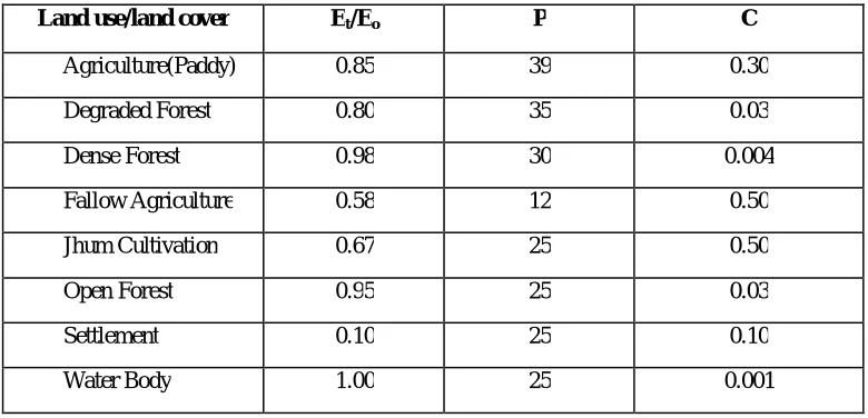
To determine the spatial distribution of average annual soil loss, the parameters of MMF models, viz., A, C, Et/Eo, and RD for land use/cover map were calculated using typical values of plant parameters (Morgan et al., 1984), and are presented in Tables 1 and 2. The parameters R and Rn were calculated from the daily rainfall data. Attribute maps were prepared for MS, BD, Rooting depth (RD), Et/Eo and land use/land cover map in GIS environment. All these were used as inputs for calculation of final value of Rc. Ro was computed using annual rainfall (R) and number of rainy days (Rn). The Soil detachability (K) and percent permanent interception and stem (or stream) flow (A) maps were prepared in GIS environment. Finally, the values of detachment rate and transport capacity of runoff were computed for each pixel, and the minimum values from each of them were used for preparation of soil erosion map.
Table 1 Typical value of different soil parameters for use in MMF Model
Soil Type MS BD K
Clay 0.45 1.1 0.02
Clay Loam 0.40 1.3 0.04
Silty Loam 0.30 1.3 0.03
Sandy Loam 0.28 1.2 0.03
Silt Loam 0.25 1.3 0.04
Loam 0.20 1.3 0.04
Fine Sand 0.15 1.4 0.20
Sand 0.08 1.5 0.70
Table 2 Typical values of plant parameter for use in MMF Model
Land use/land cover Et/Eo P C
Agriculture(Paddy) 0.85 39 0.30
Degraded Forest 0.80 35 0.03
Dense Forest 0.98 30 0.004
Fallow Agriculture 0.58 12 0.50
Jhum Cultivation 0.67 25 0.50
Open Forest 0.95 25 0.03
Settlement 0.10 25 0.10
Technology, Nirjuli - 791109, Arunachal Pradesh, India
2.7 Universal Soil Loss Equation (USLE)
USLE is defined as follows:
A
R
K
LS
C
P
(7)where A is the average annual soil loss per unit area (t ha-1yr-1), an estimate of the average annual sheet plus rill erosion from rainstorms for field size upland area; R is the rainfall-runoff erosive factor for a specific location, usually expressed as average annual erosion index units (MJ-mm-ha-1-h-1); K is the soil erodibility factor for a specific soil horizon, expressed as soil loss per unit of area per unit of R for a unit plot (t ha h ha-1 MJ-1); L is the dimensionless slope-length factor, and not the actual slope length, expressed as the ratio of soil loss from a given slope length to that of from a 22.13 meter slope length under same conditions; S is a dimensionless slope-steepness factor and not the actual slope steepness expressed as the ratio of soil loss from a given slope steepness to that of from a 9 percent slope under the same conditions; C is a dimensionless cover and management or cropping factor, expressed as a ratio of the soil loss from the condition of intersects to that of from tilled continuous fallow; P is a dimensionless conservation practice factor, expressed as a ratio of the soil loss with practices, such as contouring, strip cropping, or terracing to that of farming from a up-and-down slope. To determine the spatial distribution of average annual soil loss in the Dikrong river basin, cell- based USLE parameters in the specified 100 m × 100 m cells were multiplied for each year separately, i.e. 1988 to 2004. The annual soil losses were grouped into different scales of priority (Singh et al., 1992).
2.8 Development of model database for USLE
Rainfall erosivity (R)
Rainfall data of 17 years (1988-2004) collected from Rural Works Department (RWD), Itanagar, Papumpare, were used for calculating the R-factor. Since rainfall intensity of the watershed could not be estimated in the absence of a recording type raingauge, monthly values were used in annual calculations using the following relationship (Wischmeier and Smith; 1978):
12
1
) 08188 . 0 ) / ( log 5 . 1 ( 10 2
10
735
.
1
i
p pi
R
(8)where R is the rainfall erosivity factor (MJ-mm-ha-1-h-1-yr-1), Pi is the monthly rainfall (mm), and P is the annual rainfall (mm). Since there is only one raingauge station in the study area, one R factor was calculated and used for the watershed.
Soil erodibility factor (K)
The K-factor was calculated using the following relationship (Foster et. al., 1981):
K
2
.
8
10
7
M
1
.
14
12
a
4
.
3
10
3
b
2
3
.
3
10
3
c
3
(9)Technology, Nirjuli - 791109, Arunachal Pradesh, India
soil permeability class was considered moderate whose value was 3. The magnitude and spatial distribution of soil erodibility is seen to range from 0.039 to 0.054.
Topographic factor (LS)
The topography affects the runoff characteristics and transport processes of sediment on watershed scale. It consists of slope length and slope steepness factors.
(a) Slope length factor (L)
The L-factor was calculated using the following the relationship (McCool et al., 1989):
L
/
22.13
m(10)
where L is the slope length factor; λ is the field slope length (m); m is the dimensionless exponent that depends on slope steepness, being 0.5 for slopes exceeding 5 percent, 0.4 for 4 percent slopes and 0.3 for slopes less than 3 percent. The percent slope was determined from digital elevation model (DEM), using a grid size of 100 m as the field slope length (λ) which is consistent with the works of Pandey et al. (2007), Onyando et al. (2005), Fistikoglu and Harmancioglu (2002), and Jain et al. (2001).
(b) Slope steepness factor (S)
The S- factor was calculated for slope length longer than 4 m as (McCool et. al., 1987):
S = 10.8 sinθ + 0.03 for slopes < 9 per cent (11a)
S =16.8 sinθ – 0.50 for slopes ≥ 9 per cent (11b)
where S is the slope steepness factor (nondimensional) and θ is the slope angle in degree. Topographic factor
(LS) ranged from 0.1 to 53.1.
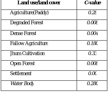
Crop management factor (C)
The land use/land cover map was derived from the satellite images (Pandey et al., 2008) to assign C and P factors for different land use classes. The magnitude and spatial distribution of crop management factor are presented in Table 3, respectively and are found to range from 0.004 to 1.00.
Table 3 Crop management factor for different land use/land cover class (USLE)
Land use/land cover C-value
Agriculture(Paddy) 0.28
Degraded Forest 0.008
Dense Forest 0.004
Fallow Agriculture 0.180
Jhum Cultivation 0.33
Open Forest 0.008
Settlement 0.00
Technology, Nirjuli - 791109, Arunachal Pradesh, India
Conservation practice factor (P)
In the study area, no major conservation practice is followed. The values for P-factor were assigned as 0.28 for area under paddy cultivation and 1.0 for other area (Rao, 1981).
III. RESULTS AND DISCUSSION
To determine the spatial distribution of average annual soil loss in the Dikrong river basin, the MMF parameters were estimated in the specified 100 m × 100 m cells. Soil losses were estimated separately for each year, from 1988 to 2004, and these were grouped into different scales of priority as suggested by Singh et al. (1992). To estimate the soil erosion due to splash detachment, the annual rainfall and 30 mm.h-1 intensity of rainfall were used as inputs.
3.1 Soil Loss estimation using MMF
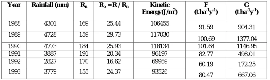
Based on 17 years daily rainfall data, the estimated maximum and minimum values of kinetic energy were 118134 and 56821 (J m-2) for 1990 and 2001, respectively, and the estimated average annual soil loss was 75.66 tha-1y -1
(Table 4). The analysis for the years 1988-2004 shows that the soil loss was 101.64 tha-1y-1 in 1990, the year of high rainfall (4772 mm). The lowest value of soil loss was 48.89 tha-1y-1 in 2001 when rainfall was only 2296 mm. Since the MMF Model considers the minimum of the values of soil losses between splash detachment (F) and overland flow (Q), the wide variations in soil losses for different years is mainly due to variation in rainfall pattern. Furthermore, the soils ranging from sandy loam to sand in texture exhibit low soil moisture storage capacity, less rooting depth, poor crop management, and high relief contributing to high volume of overland flow, and thus, higher transport capacity of overland flow. These conditions contribute to high soil losses in the study area. The average annual soil loss computed by MMF model is 32.6 percent higher than that due to USLE (Dabral et al., 2008) for the Dikrong river basin.
Since the soil loss due to MMF is greater than 20 t ha-1 yr-1, the soil loss maps were regrouped into three classes (Singh et al., 1992) as presented in Table 5. It is seen from the table that 2.8, 57.9, and 39.3 percent areas of the basin fall in very high, severe, and very severe priority classes, respectively. The priority classes for soil erosion are identified and shown in Table 5.
An investigation of the sediment yield data shows that the 39.3 percent area of the watershed is falling under very severe erosion class (>80 tha-1y-1). The results obtained from MMF model show that all the Dikrong river basin requires immediate conservation measures. Its spatial distribution shows that the most erosive areas are located on steep slope, either abandoned after Jhum cultivation or with sparse vegetation. Saha et al. (2002) reported that the Himalaya is undergoing rapid uplift at a rate between 0.5 to 4 mm per year and consequently experiencing rapid erosion causing deposition of thick pile of terrigeneous sequences.
Table 4 Estimated Rn, R0, kinetic energy and MMF estimated average annual soil loss
Year Rainfall (mm) Rn Ro = R / Rn Kinetic Energy(J/m2)
F (tha-1y-1)
G (tha-1y-1)
1988 4301 169 25.44 106455
91.59 904.31
1989 4728 159 29.73 117030
100.69 1377.04
1990 4773 184 25.93 118134 101.64 1146.95
1991 3887 191 20.34 96197 82.77 498.01
1992 2827 170 16.62 69959 60.19 172.25
1993 3779 155 24.37 93526
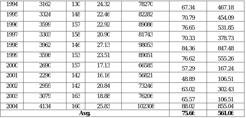
Technology, Nirjuli - 791109, Arunachal Pradesh, India
1994 3162 130 24.32 78270
67.34 467.18
1995 3324 148 22.46 82282
70.79 454.09
1996 3599 157 22.92 89086
76.65 531.85
1997 3303 158 20.90 81743
70.33 378.73
1998 3962 146 27.13 98053
84.36 847.48
1999 3598 153 23.51 89051
76.62 555.26
2000 2690 157 17.13 66585
57.29 167.24
2001 2296 142 16.16 56821
48.89 106.51
2002 2959 142 20.84 73246
63.02 302.43
2003 3079 163 18.88 76206
65.57 106.51
2004 4134 160 25.83 102308 88.02 855.04
Avg. 75.66 561.06
Table 5 Area under different classes of soil erosion in Dikrong river basin (MMF)
Sediment yield, (tha-1y-1) Percent area Soil erosion class
20-40 2.8 Very high
40-80 57.9 Severe
>80 39.3 Very severe
3.2 Estimation of Soil loss using USLE
The USLE parameters were estimated and multiplied in the specified 100 m
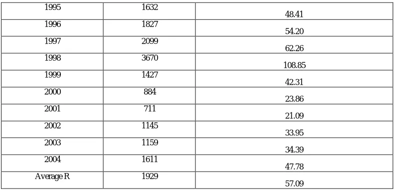
100 m cells to estimate the average annual soil loss. The average R-factor was observed to be 1929 MJ mm ha−1h−1yr−1. Its highest value (5826 MJ mm ha−1h−1yr−1) was observed in 1989 when the total rainfall and rainy days were 4728 mm and 135 days, respectively (Table 6). The lowest value (711 M J mm ha−1h-yr−1) occurred in 2001 when the total rainfall and rainy days were 2440 mm and 120 days, respectively. However, in this study, the spatial distribution of R was assumed to be uniform.The average annual soil loss from the study basin is computed as 57.06 t ha-1yr-1; the highest soil loss (172.81 tha -1
yr-1) occurred in 1990, the year of high rainfall (4772 mm) and the lowest (21.09 tha-1yr-1) in 2001, the year of low rainfall (2296 mm). High values of LS-factor and slope, the important factors causing erosion, lie in the lower part of the basin.
Table 6 Estimated R-factor and average annual soil loss (USLE)
Year R-factor Average annual soil loss (tha-1y-1)
1988 1892
56.13
1989 5825
72.98
1990 2460
172.81
1991 1457
43.22
1992 914
27.10
1993 1963
58.23
1994 2120
Technology, Nirjuli - 791109, Arunachal Pradesh, India
The priority classes for soil losses in the study area were regrouped into six classes (Singh et al., 1992) as shown in Table 7. It is observed from table that 24.0, 12.4, 19.7, 18.5, 7.3 and 18.1 percent areas of the study basin fall under slight, moderate, high, very high, severe, and very severe erosion classes, respectively.It also indicates the requirement of soil conservation in the study area.
Table 7 Area under different classes of soil erosion in Dikrong river basin (USLE)
Sediment yield (tha-1y-1)
Percent area Soil erosion class
0-5 24.0 Slight
5-10 12.4 Moderate
10-20 19.7 High
20-40 18.5 Very high
40-80 7.3 Severe
>80 18.1 Very severe
3.3 Comparison of soil losses obtained by using MMF and USLE models
As stated above, the Dikrong river basin has not been gauged for soil erosion, and therefore, the verification of above results was not possible. Though, the soil loss estimation using the above models matched with each other qualitatively, but the results differed in quantitative estimation. Apparently, the soil loss from Dikrong river basin using the MMF model is > 20 t ha-1y-1, and the maximum and minimum soil loss obtained from both the models occurred in 1990 (rainfall = 4773 mm) and 2001 (rainfall= 2296 mm), respectively. The results of the USLE model seem to be more reasonable as it accounts for the topographical characteristics in soil loss estimation. Similar USLE model results are reported by Dabral et al. (2008) and Pandey et al.(2007). On the other hand, the soil loss from MMF model was calculated using the minimum values of detachment rate (F) used in preparation of soil erosion map, and thus, it did not account for the ground slopes. As seen, the 56.1 percent area of watershed belongs to the category of soil loss < 20 t ha-1 yr-1, which is tolerable for the hilly terrain where the natural rate of soil loss is high (Morgan, 1986).To summarize, the results of USLE model show that 43.9 percent area exhibits a soil loss > 20 t ha-1y-1 and 18.10 percent area falls under very severe erosion category, which may be attributed to high rainfall coupled with fragile rock and high relief prevalent in the study area. The average annual soil loss computed by USLE in this study is 10.66 % higher than that due to USLE (Dabral et al., 2008) for the Dikrong river basin. The higher soil loss in this study may be because of the finer grid cell resolution (i.e. 100 × 100 m) as compared to Dabral et al. (2008).
1995 1632
48.41
1996 1827
54.20
1997 2099
62.26
1998 3670
108.85
1999 1427
42.31
2000 884
23.86
2001 711
21.09
2002 1145
33.95
2003 1159
34.39
2004 1611
47.78
Average R 1929
Technology, Nirjuli - 791109, Arunachal Pradesh, India
IV. CONCLUSIONS
The following conclusions can be drawn from the study:
1. The estimated average annual soil loss from MMF model is 75.66 t ha-1y-1 from the Dikrong river basin. It varies in the range of 48.89 to 101.64 tha-1y-1.
2. The results from the MMF model shows that approximately 2.8 % of the study area lies in very high, 57.9 % in severe, and 39.3 % in very severe (>80 tha-1y-1 ) soil erosion zones.
3. The average annual soil loss from USLE is 57.06 t ha-1y-1, and it varies in the range of 21.09 to 172.81 tha-1y -1
.
4. According to USLE application, 18.1% of the study area lies in the very high priority (>80 tha-1y-1), 7.3 % in the range 40-80 tha-1y-1, 18.5 % in 20-40 tha-1y-1, 19.7 % in 10-20 tha-1y-1, 12.4 % in 5-10 tha-1y-1, and 24.0 % in very low priority zone of 0-5 tha-1y-1.
5. Finally, the results of both the MMF and USLE models indicate that major parts of the basin lie in very high, severe, and very severe zones and need immediate attention from soil conservation view point.
6. USLE model results are more realistic and can be adopted in the hilly Himalayan Watersheds.
REFERENCES
1. Baba, S.M.J. and Yusof, K.W. (2001). Modeling soil erosion in tropical environments using remote sensing and geographical informations systems, Hydrologic Sci J.46(1), 191–198.
2. Barrow, C.J. (1991). Land Degradation, Cambridge University Press, Cambridge.
3. Dabral, P.P., Baithuri, N. and Pandey, A. (2008). Soil erosion assessment in a hilly catchment of north eastern India using USLE, GIS and remote sensing. Water Resour. Manage (Springer). DOI: 10.1007/s11269-008-9253-9.
4. Dabral, P.P., Murry, R.L. and Lollen, P (2001). Erodibility status under different land uses in Dikrong river basin of Arunachal Pradesh. Indian J. Soil Cons. 29 (3), 280-282.
5. Dhruvanarayana, V.V. and Rambabu (1983) Estimation of Soil loss in India. J Irr. Drainage Eng 109(4), 419-433.
6. Dickinson, A. and Collins, R. (1998) Predicting erosion and sediment yield at the catchment scale. Soil erosion at multiple scales. CAB Int 317–342.
7. Fistikoglu, O., and Harmancioglu, N. B., 2002., Integration of GIS with USLE in assessment of soil erosion. Kluwer Academic Publishers.Water Resources Management 16: 447–467.
8. Foster, G.R., Mc Cool, D.K., Renard, K.G., and Moldenhauer, W.C., 1991., Conversion of the Universal soil loss equation to SI Metric Units, J. Soil & Water Conserv. 36:355-359.
9. Jain, S.K., Kumar, S. and Varghese, J. (2001). Estimation of soil loss for a Himalayan watershed using GIS technique. Water resources
management. (15), 41-54.
10. Jain, M.K. and Kothyari, U.C. (2000). Estimation of soil erosion and sediment yield using GIS. Hydrological Sciences J. 45 (5), 771-786. 11. Jasrotia, A.S., Dhiman S.D. and Aggarwal, S.P. (2002). Rainfall-runoff and soil erosion modeling using remote sensing and GIS technique-A
case study of tons watershed. J. Indian soc. Remote Sensing. 30(3), 167-180.
12. Jose, C.S. and Das, D.C., (1982). Geomorphic prediction models for sediment production rate and intensive priorities of watershed in Mayurakshi catchment. Proceedings of the international symposium on Hydrological Aspects of Mountainous Watershed held at School of Hydrology, University of Roorke.15-23.
13. Julien, P.Y. and Frenette, M. (1987). Macroscale analysis of upland erosion. Hydrol Sci J 32(3), 347–358.
14. Julien, P.Y. and Gonzales del Tanago, M. (1991) Spatially varied soil erosion under different climates. Hydrol Sci J 36(6), 511–524.
15. Kirkby, M.J. (1976). Hydrogical slope models: the influence of climate. In: Derbyshire, E. Ed. , Geomorphology and Climate. Wiley, London, pp. 247–267.
16. Ives, J.D. and Messerli, B. (1989). The Himalayan Dilemma: Reconciling Development and Conservation, Routledge, London.
17. Meyer, L.D. and Wischmeier, W.H. (1969). Mathematical simulation of the process of soil erosion by water.Transactions of the American Society of Agricultural Engineers. (12), 754–758 and 762.
18. McCool, D.K., Foster, G.R., Mutchelor, C.K and Mayer, L.D. (1987) Revised slope length factor for the Universal Soil Loss Equation. Trans. ASAE. (32), 1387-1396.
19. Misra, N, Satyanarayana, T. and Mukherjee, R.K., (1984) Effect of topo elements on the sediment production rate from subwatersheds in upper Damodar valley. Journal of Agricultural Engg. (ISAE). 21 (3), 65-70.
20. Morgan, R.P.C. (2000). A simple approach to soil loss prediction: a revised Morgan–Morgan–Finney model. Catena. (44), 305–322. 21. Morgan, R.P.C. (1986). Soil Erosion and Conservation. Longman, England.
22. Morgan, R. P. C., Morgan, D. D. V. and Finney, H. J. (1984). A predictive model for the assessment for the soil erosion risk, Journal of Agriculture Engineering Research 30, 245–253.
23. Onyando, J.O., Kisoyan, P. and Chemelil, M.C. (2005). Estimation of potential soil erosion for river perkerra catchment in Kenya. Water Resources Management. (19),133–143.
Technology, Nirjuli - 791109, Arunachal Pradesh, India
25. Pandey, A., Dabral, P.P., Chowdary, V.M. and Yadav, N.K. (2008). Landslide hazard zonation using remote sensing and GIS: a case study of Dikrong river basin, Arunachal Pradesh, India. Environmental Geology. 54:1517–1529.
26. Rao, Y.P., 1981., Evaluation of cropping management factor in Universal soil Loss Equation under natural Rainfall Condition of Kharagpur, India. Proceedings of Southeast Asian Regional Symposium on problems of soil erosion and Sedimentation, Asian Institute of Tedchnology, Bangkok. 241-254 pp.
27. Renschler C, Diekkruger B, and Mannaerts C. (1997). Regionalization in surface runoff and soil erosion risk evaluation, in Regionalization of Hydrology. IAHS Publishers, UK, 254, 233–241.
28. Saha, A. K., Gupta, R. P., and Arora, M. K. (2002). GIS-based Landslide hazard Zonation in the Bhagirathi (Ganga) Valley, Himalayas. International Journal of Remote Sensing. 23 (2), 357-369.
29. Satpathy, K.K. and Dutta, K.K. (1999). Re-vegetation of eroded hill slopes- an experience with geo-jute in Arunachal Pradesh. Indian J Soil Cons. 27(3), 227-233.
30. Sfeir-Younis A. (1986). Soil Conservation in Developing Countries, Western Africa Projects Department/ The World Bank, Washington, DC. 31. Singh, G., babu, R. Narain, P., Bhusan, L.S. and Abrol, I.P. (1992), Soil Erosion rates in India. Journal of Soil and water Conservation 47 (1):
97-99.
32. Singh, S. (1999). A Resources Atlas of Arunachal Pradesh. Government of Arunachal pradesh. P-141-143.
33. Thampapillai, D.A. and Anderson, J.R. (1994). A review of the socio-economic analysis of soil degradation problem for developed and developing countries. Review of Marketing and Agricultural Economics. (62), 291-315.
34. Williams, J.R. and Berndt H.D. (1972) Sediment yield computed with universal equation. J Hydrol Div, ASCE 98(12), 2087–2098. 35. Williams, J.R. and Berndt, H.D. (1977). Sediment yield prediction based on watershed hydrology. Trans ASAE : 1100– 1104.
36. Wilson, J.P. and Gallant J.C. (1996) EROS: A grid-based program for estimating spatially distributed erosion indices. Comp Geosci 22(7), 707– 712.
37. Wischmeier, W.H. and Smith, D.D. (1978). Predicting rainfall erosion losses. USDA Agricultural Research Services Handbook 537. USDA, Washington, DC.
38. Wu, S, Li J and Huang G (2005). An evaluation of grid size uncertainty in empirical soil loss modelling with digital elevation models.