ABSTRACT
LEVIS, JAMES WILLIAM. A Mathematical Programming Life-Cycle Assessment Model for Solid Waste Management Decision Making. (Under the direction of Dr. Ranji S. Ranjithan and Dr. Morton A. Barlaz.)
Solid waste management (SWM) is an integral component of civil infrastructure and the broader U.S. economy and policy makers have taken an increasing interest in reducing environmental impacts associated with SWM. In the future, greenhouse gas (GHG)
mitigation policies that affect the U.S. energy mix as well as the cost of energy and emissions could significantly impact the strategic direction of SWM. As such, SWM systems must proactively adapt to changing waste composition, policy requirements, and an evolving energy system to cost-effectively and sustainably manage future solid waste.
SWM life-cycle assessment (LCA) models integrated into an optimization framework can simultaneously consider all possible waste collection and treatment alternatives to find the combination of technologies that optimizes environmental and economic objectives. Such a framework must be able to represent multi-stage decisions to consider the changes to the SWM system over time.
The objectives of this research are: to develop the Solid Waste Optimization Life-cycle Framework (SWOLF); to illustrate the use of the framework to analyze the economic and environmental impacts and trade-offs associated with SWM systems based on future changes to waste generation, waste composition, and energy projections; and to analyze the
illustrative results to understand how variations in the energy system, GHG policy, and SWM policy affect optimal SWM decisions. SWOLF uses a mixed integer linear programming model to determine optimal SWM strategies while considering the interdependencies among processes in the SWM system. SWOLF is generalizable to include numerous SWM treatment facilities and collection options, and solves in less than two hours using readily available hardware and software.
may be counterproductive towards reducing GHG emissions in some instances. Relatedly, the model found that SWM strategies designed to reduce GHG emissions were more cost effective at reducing GHG emissions than SWM strategies designed to increase diversion, which indicates that SWM decision makers should focus on the environmental impacts they wish to reduce, instead of using potentially problematic proxies such as landfill diversion. The case study provided numerous insights that were only possible through the use of a stage-wise life-cycle optimization framework. For example, both the diversion maximizing and GHG minimizing scenarios showed stage-wise switching of anaerobic digestion (AD) and composting throughputs based on changes to waste composition and generation.
The model was then used to investigate the effects of energy, GHG, and SWM policies on optimal SWM strategies. This case study required integrating SWOLF with energy system modeling results to investigate how changes in GHG policy and the energy system affect SWM system performance. Minimum cost SWM strategies with GHG emission and
A Mathematical Programming Life-Cycle Assessment Model for Solid Waste Management Decision Making
by
James William Levis
A dissertation submitted to the Graduate Faculty of North Carolina State University
in partial fulfillment of the requirements for the degree of
Doctor of Philosophy
Civil Engineering
Raleigh, North Carolina 2013
APPROVED BY:
_______________________________ ______________________________
Morton A. Barlaz Ranji S. Ranjithan
Committee Co-Chair Committee Co-Chair
________________________________ ________________________________
Joseph F. DeCarolis E. Downey Brill
ii
DEDICATION
BIOGRAPHY
iv
ACKNOWLEDGMENTS
Letting your mind play is the best way to solve problems. -Bill Watterson
I would like to take this opportunity to thank everyone whose advice and support has helped me throughout this endeavor. I would like to thank the Environmental Research and
TABLE OF CONTENTS
LIST OF TABLES ... viii
LIST OF FIGURES ... ix
SYMBOLS USED ... xiv
1 INTRODUCTION ... 1
2 A MULTISTAGE OPTIMIZATION MODEL FOR LIFE-CYCLE ASSESSMENT-BASED INTEGRATED SOLID WASTE MANAGEMENT ... 4
2.1 Introduction ... 4
2.2 Integrated Solid Waste Management Modeling Framework ... 6
2.2.1 Life cycle assessment framework for solid waste management ... 6
2.2.2 Mass flow modeling ... 8
2.2.3 Facility capacity modeling ... 13
2.2.4 Cost modeling ... 14
2.2.5 Environmental emissions modeling ... 15
2.2.6 Solid waste management policy requirements ... 17
2.3 Illustrative Integrated Solid Waste Management System ... 18
2.4 Mathematical Expressions for the Integrated Solid Waste Management Model . 21 2.4.1 Mass flow expressions ... 21
2.4.2 Facility capacity expressions ... 24
2.4.3 Cost expressions ... 32
2.4.4 Environmental emissions expressions ... 34
2.4.5 Solid waste management policy expressions ... 34
2.5 Results and Discussion ... 35
vi
2.5.2 Computational performance ... 39
2.5.3 Implications, conclusions, and future work ... 40
References ... 41
3 USE OF THE SOLID WASTE OPTIMIZATION LIFE-CYCLE FRAMEWORK TO MINIMIZE FUTURE COST AND ENVIRONMENTAL IMPACTS FROM SOLID WASTE MANAGEMENT ... 43
3.1 Introduction ... 43
3.2 Problem Description and Modeling Approach ... 44
3.2.1 Representative Solid Waste Management System ... 45
3.2.2 Optimization Modeling ... 49
3.2.3 Solid Waste Management Scenarios ... 50
3.3 Results and Discussion ... 51
3.3.1 Mass Flows, Costs, and GHG Emissions ... 51
3.3.2 GHG Mitigation Costs ... 55
3.3.3 Cost, Diversion, and GHG Emission Trade-offs ... 56
3.3.4 Discussion ... 58
References ... 60
4 OPTIMAL SOLID WASTE MANAGEMENT STRATEGIES FOR PROACTIVELY ADAPTING TO SOLID WASTE MANAGEMENT, ENERGY, AND CLIMATE POLICIES ... 62
4.1 Introduction ... 62
4.2 Policy Modeling ... 64
4.2.1 Energy System and GHG Policy ... 64
4.2.2 Solid Waste Management Policy ... 65
4.4 Scenarios and Cases... 68
4.5 Results and Discussion ... 72
4.5.1 Mass Flows, Costs, and GHG Emissions ... 72
4.5.2 Discussion ... 82
References ... 84
5 CONCLUSIONS... 87
APPENDICES ... 90
APPENDIX A. Illustrative system data ... 91
APPENDIX B. Solid waste management case study system information... 96
viii
LIST OF TABLES
Table 2-1. Definition of terms used in the modeling of mass flows in a SWM
system. ...9 Table 2-2. Waste generation for the illustrative SWM system shown in Figure
2-5...18 Table 2-3. Collection schemes and their associated treatment schemes in the
illustrative example. The treatment scheme designations are formed from the destinations of mixed waste collection, MRF residuals, and ash. The illustrative system has three collection processes with six
collection schemes, as well as 17 treatment schemes (the number of
collection andtreatment schemes that include a MRF are doubled to
include the MRF_N and MRF_E alternatives). ...20 Table 2-4. Net present cost, annual GHG emissions, and diversion results for the
three illustrative scenarios. The MinCost scenario costs the least, generates the most GHG emissions, and diverts the least. The
Diversion scenario costs the most and diverts the most, while the GHG
scenario generates the least GHG emissions. ...35 Table 2-5. Solve times for a representative system using typical laptop hardware
with CPLEX and GLPK solvers. ...39 Table 4-1. Energy System Scenarios, SWM Policy Scenarios, and subsequent
cases analyzed. ...69 Table 4-2. Variation in RPS renewables requirement, and CO2 price for the RPS
and CO2 scenarios ...69 Table 4-3. Annual cost, GHG emissions and percent diversion in each stage for
the RefBase and RefEnvPol cases. The percent changes from these
LIST OF FIGURES
Figure 1-1 Generalized modeling framework showing how energy system modeling is connected to LCA models for a SWM system, and how the outputs of these models are then used as inputs into an optimizable
LCA framework to systematically analyze future SWM. ...2 Figure 2-1. Inputs and outputs for a generic waste treatment process model. Input
masses and all outputs are specified per unit mass of each waste
material. Model parameters and user inputs are used to characterize the transformation of the incoming waste mass as well as the resulting emissions, fuel use, and costs. User inputs represent the model parameters that are system-specific, which need to be specified by users, while default values are available for other model parameters. 1
Mg = 1 metric ton. ...7 Figure 2-2. An example of a set of treatment schemes that shows the potential
waste flows for all of the collected waste. The organics and recyclable collection processes are both specific collection processes. The single stream MRF, mixed waste MRF, composting, WTE, and landfill are all potential collection destinations. In this example system, there are 102 possible treatment schemes and each one belongs to at least one
collection scheme. ...11 Figure 2-3. All the treatment paths for the example shown in Figure 2-2.
Treatment schemes are produced by combining one mixed waste
treatment path with at most one of each of the recyclable and source
separated organics paths (i.e., more than one of either is not allowed). ...13 Figure 2-4. System boundary for the SWM life-cycle assessment. Gross emissions
are generated through electricity, fuel, and raw material extraction and processing, as well as directly in SWM processes. Emission offsets are produced from avoiding electricity generation, soil amendment
production, and virgin material production. Net emissions are equal to
the difference between gross and avoided emissions. ...17 Figure 2-5. System model of potential mass flows for the illustrative example.
WTE, LF, and MRF are all potential collection destinations. The residual waste collection process collects the waste mass not collected by recyclable collection. Recyclable collection requires residual waste
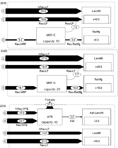
x Figure 2-6. Material flow diagrams for each stage of the Diversion scenario. The
numbers represent mass in 1000 Mg/yr. Recycling is performed using the 10,000 Mg/yr MRF_E in the first stage and a new 20,000 Mg/yr MRF_N in the second stage before a 40,000 Mg/yr WTE facility is built to meet the final 50% diversion target. G – waste generation, NRec-LF – Flow of NRec to the LF, Rec-LF – Flow of Rec to the LF, Rec-MRF – Flow of Rec to the MRF, Res-LF – Flow of MRF residual to LF, Rec-ReMfg – Flow of Rec to ReMfg, NRec-WTE – Flow of
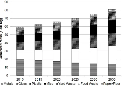
NRec to WTE, and Rec-WTE – Flow of Rec to WTE. ...38 Figure 3-1. Mass of waste generated by waste category in each stage. Waste
composition by specific waste materials is provided in Table B-1. Paper/ Fiber generation decreases by 32%, while food waste
generation increases by 108%, which indicates that different treatment
processes may be better suited to meet future SWM needs. ...45 Figure 3-2. Waste management system potential mass flow diagram. Mixed waste
collection collects all of the generated waste, while residual collection collects the remaining waste after recyclable and organics collection. Separated material from the MRFs can either be recycled or treated by WTE combustion. Bottom ash can be recycled as aggregate in
concrete, and the aluminum and ferrous in the bottom ash can be separated and recycled. The distinction between bottom and fly ash
has been removed for simplicity. ...48 Figure 3-3. Percent change in electricity cost, electricity GHG intensity, diesel
cost, and heavy-duty truck fuel efficiency based on U.S. EIA AEO 2012 reference scenario projections. Sale price of electricity is assumed to be half of cost. Prices and costs are in nominal U.S. dollars. Electricity mix and GHG emissions for generation
technologies are shown in Table B-25. ...49 Figure 3-4. Net present cost (2010 U.S. Dollars), 30-year cumulative GHG
emissions, and cumulative 30-year diversion for each of the base scenarios. Negative GHG emissions are due to electricity generation offsets (AD, landfill, WTE), material recovery offsets, and carbon
storage (AD, composting, landfill). ...51 Figure 3-5. The total mass of material entering each process in each stage for the
Min Cost, Max Diversion, and Min GHG scenarios. A landfill and SSMRF are used in all scenarios, and the Max Diversion and Min GHG scenarios both additionally use AD, composting, MWMRF, and
Figure 3-6. The annual GHG emissions from each process in each stage for the Min Cost, Max Diversion, and Min GHG scenarios. Transportation represents any transport of materials after initial curbside collection. Collection is the greatest net generator of GHG emissions in all scenarios, and remanufacturing is the greatest GHG sink in all scenarios. The Min GHG scenario has greater remanufacturing benefits than the Max Diversion scenario because only materials with
net GHG benefits are recycled in the former case. ...53 Figure 3-7. Annual GHG mitigation cost and GHG reduction for Min Cost, Max
Diversion, and Min GHG scenarios compared to the business-as-usual (BAU) scenario. Negative mitigation costs indicate that there are cost savings associated with the GHG reductions. The bars represent GHG reductions while the lines represent mitigation costs. Only the GHG reductions are shown for the Max Diversion scenario because it increases GHG emissions relative to the BAU scenario. Costs are in
nominal 2010 U.S. dollars. ...56 Figure 3-8. Trade-offs for cost vs. 30 yr diversion (C\D) and cost vs. 30 yr GHG
emissions (C\G). The C\D points represent the system achieving the maximum diversion for the specified cost, and the C\G points represent the system achieving minimum GHG emissions at the specified cost. Cost is in 2010 U.S. dollars. (Div: Diversion, GHG:
Greenhouse gas emissions). ...57 Figure 3-9. Mass throughputs and GHG emissions from each process in each stage
of the trade-off scenario that minimized GHG emissions with a cost 10% greater than the Min Cost scenario. White circles show
corresponding non-zero throughputs for Min Cost scenario. Net present cost was $87 million, 30 yr GHG emissions were -710,000
MTCO2e, and the 30 yr diversion rate was 44%. ...58 Figure 4-1. Waste management system mass flow diagram representing potential
material flows through the wate management system. Mixed waste collection collects all of the generated waste, while residual collection collects the remaining waste after recyclable and/or organics
collection. Separated material from the MRFs can either be recycled or treated by WTE combustion. Bottom ash can be recycled as aggregate in concrete, and the aluminum and ferrous in the bottom ash can be separated and recycled. The distinction between bottom and fly ash
xii Figure 4-2. Change in energy system parameters from 2010 baseline based on
energy modeling described in Section 4.2.1. Most of the variation in electricity GHG intensity is due to fuel switching from coal to natural gas or renewables. Transportation cost changes are small since diesel vehicles comprise the majority of transport in all scenarios. (vkmt =
vehicle kilometer traveled) ...71 Figure 4-3. The total mass of material entering each process in each stage for the
RefBase, RPSBase, LowNGBase, and CO2Base cases. All the energy scenarios for the base case had the same throughputs (except for minor
differences [< 1%] in the CO2Base case). ...73 Figure 4-4. The total mass of material entering each process in each stage for the
RefEnvPol case. ...73 Figure 4-5. The total mass of material entering each process in each stage for the
RPSEnvPol case. ...74 Figure 4-6. The total mass of material entering each process in each stage for the
LowNGEnvPol case. ...74 Figure 4-7. The total mass of material entering each process in each stage for the
CO2EnvPol case. ...74 Figure 4-8. The annual GHG emissions from each process in each stage for the
RefBase case. The GHG emissions for all base cases are similar. Transportation represents any transport of materials after initial
curbside collection. ...75 Figure 4-9. The annual GHG emissions from each process in each stage for the
RPSBase case. The GHG emissions for all base cases are similar and the GHG emissions. Transportation represents any transport of
materials after initial curbside collection. ...75 Figure 4-10. The annual GHG emissions from each process in each stage for the
LowNGBase case. The GHG emissions for all base cases are similar and the GHG emissions. Transportation represents any transport of
materials after initial curbside collection. ...76 Figure 4-11. The annual GHG emissions from each process in each stage for the
CO2Base case. The GHG emissions for all base cases are similar and the GHG emissions. Transportation represents any transport of
Figure 4-12. The annual GHG emissions from each process in each stage for the RefEnvPol case. Transportation represents any transport of materials
after initial curbside collection. ...77 Figure 4-13. The annual GHG emissions from each process in each stage for the
RPSEnvPol case. Transportation represents any transport of materials
after initial curbside collection. ...77 Figure 4-14. The annual GHG emissions from each process in each stage for the
LowNGEnvPol case. Transportation represents any transport of
materials after initial curbside collection. ...78 Figure 4-15. The annual GHG emissions from each process in each stage for the
CO2EnvPol case. Transportation represents any transport of materials
after initial curbside collection. ...78 Figure 4-16. The percent change in annual cost (A) and GHG emissions (B) for
each stage (after the initial stage, where the systems are the same) and case compared to the corresponding Reference energy scenario case (i.e., the Min Cost cases are compared to the RefBase case, and the EnvPol cases are compared to the RefEnvPol case). Percent change shown in GHG emissions is actually negative percent change because the net GHG emissions in all cases were negative (i.e., negative values
xiv
SYMBOLS USED
αwm_in,wm_out,ws,tp Mass of waste materialwm_out exiting treatment processtp in waste streamws per incoming mass of waste materialwm_in. Used to represent the separation efficiency in MRFs and ash fraction in WTE processes.
βwm,t The proportion of waste materialwm in the generated wastein stage t. ∑ .
γcs,cp,tp Indicator coefficient that equals 1 if treatment processtp is the collection destination for collection processcp in collection schemecs, and equals 0 otherwise.
εtp,wm The utilization cost coefficient for waste material wm in treatment process tp ($/Mg).
εcs,wm,cp The utilization cost coefficient for waste material wm in collection scheme cs and collection process cp ($/Mg).
ξi,proc,wm,t The emission factor for pollutant or impact i for waste material wm from
process proc in stage t (kg/Mg or MJ/kg).
ρcap The expansion cost coefficient for capital treatment processcap
($/Mg·yr-1).
σcap The build cost coefficient for capital treatment processcap ($/Mg·yr-1). φwm,scp,t The maximum collection separation efficiency of waste materialwm
collected via specific collection processscp in stage t (0 ≤ φwm,scp,t ≤ 1). τts,tp,tp_up,ws Indicator coefficient that equals 1 if waste streamws is sent to treatment
processtp from upstream treatment processtp_up in treatment scheme ts, and equals 0 otherwise.
A/P Economic conversion factor from a present payment to a series of annual payments.
actCapcap_e The amount of existing capacity in the initial stage for existing capital treatment process cap_e (Mg/yr).
Bcap_n,t A binary variable that equals 1 if treatment process cap_n is built in stage t and 0 otherwise.
buildCostcap_n,t The build cost of new capital treatment processcap_n in stage t ($). cap The capital treatment process index.
CAP The set of capital treatment processes. A subset of TP and the union of
CAP_E and CAP_N.
CAP_E The set of existing capital treatment processes and a subset of CAP. In the illustrative example in Chapter 2 CAP_E = {MRF_E}.
cap_n The new capital treatment process index.
CAP_N The set of new treatment processes and a subset of CAP. In the illustrative example in Chapter 2 CAP_N = {MRF_N, WTE}.
capCostproc The total capital cost for treatment processproc ($).
cp The collection process index.
CP The set of collection processes and a subset of PROC. In the illustrative example in Chapter 2 CP = {MWC, CRC, RWC}.
CPcs The set of collection processes in collection schemecs and a subset of CP.
In the illustrative example in Chapter 2 CP mwc-lf and CP mwc-wte = {MWC};
and CP rwc-lf and CP rwc-wte = {CRC, RWC}.
cs The collection scheme index.
CS The set of collection schemes. In the illustrative example in Chapter 2 CS = {{(MWC-LF)}, {(MWC-WTE)}, LF), (CRC-MRF)}, {(RWC-WTE), (CRC-MRF)}}.
Dcap,t A binary variable that equals 1 if capital treatment processcap is
decommissioned in stage t and 0 otherwise.
divTargett The diversion target in stage t.
Ecap,t A binary variable that equals 1 if capital treatment processcap is
expanded in stage t and 0 otherwise.
expandCostcap,t The total expansion cost of capital treatmentprocesscap ($). FTP The final stage. In the illustrative example in Chapter 2 FTP = 3.
Fcap,t A binary variable that equals 1 if capital treatment processcap has a
currently active expansion and is not expanded in stage t and equals 0 if there is an expansion in stage t.
i The pollutant and environmental impact index.
I The set of pollutant and environmental impacts. In the illustrative example in Chapter 2 I = {GWP}.
initT The initial stage.
lf The landfill treatment process index.
LF The set of landfill treatment processes. In the illustrative example in Chapter 2 LF = {ALF, LF}.
xvi
M A sufficiently large positive constant.
minbldcapcap_n The minimum possible capacity that can be built for new capital treatment process cap_n (Mg/yr).
minexpcapcap The minimum possible capacity that can be expanded for capital treatment process cap after it has been built (Mg/yr).
Masst Total mass of waste generated in stage t (Mg).
mwcp The mixed waste collection process index in collection schemecs.
MWCPcs The set of mixed waste collection processes in collection schemecs and a
subset of CPcs. In the illustrative example in Chapter 2 MWCPmwc-lf =
MWC; MWCPmwc-wte = MWC; MWCPrwc-lf = RWC; and MWCPrwc-wte =
RWC.
opCostproc The total operating cost for capital treatment processproc ($).
P/A Economic conversion factor from a series of annual payments to a single present payment.
P/F Economic conversion factor from a single future payment to a single present payment.
proc The process index.
PROC The set of all processes. The union of CP and TP. In the illustrative example in Chapter 2 PROC = {MWC, RWC, CRC, MRF_E, MRF_N, WTE, LF, ALF}.
procAlivecap,t,T An indicator coefficient that equals 1 if t + lifecap ≤ T,and 0 otherwise. procExistcap_e,T An indicator coefficient that equals 1 if initT + remLifecap_e ≤ T,and 0
otherwise.
r The discount rate used in economic conversion factors. In the illustrative example in Chapter 2 r = 0.05.
remLifecap_e The remaining number of stages for which an existing capital treatment process cap_e is active without an expansion.
rptCostcap The net present cost of repeated builds of capital treatment processcap in
perpetuity ($).
scp The specific collection process index.
SCPcs The set of specific collection processes that collect waste streams other
than the mixed waste (e.g., recyclables or organics) in collection scheme cs and a subset of CPcs. In the illustrative example in Chapter 2 SCP mwc-lf
and SCP mwc-wte = Ø; and SCP rwc-lf and SCP rwc-wte = CRC.
T The stage index and an alias for t.
totCost The net present cost of the system ($).
totEmisi The total emissions of pollutant or impact i (kg or MJ).
tp The treatment process index.
TP The set of treatment processes and a subset of PROC. In the illustrative example in Chapter 2 TP = {ALF, LF, MRF_E, MRF_N, WTE}.
tp_up The upstream treatment process and an alias for tp.
TPts The set of treatment processes in treatment scheme ts and a subset of TP.
In the illustrative example in Chapter 2 TPL-- ={LF}; TPW-A ={WTE,
ALF}; TPW-L ={WTE, LF}; TPLL- ={LF, MRF}; TPLWA ={LF,
MRF,WTE,ALF}; TPLWL ={LF, MRF,WTE}; TPWLA ={LF,
MRF,WTE,ALF}; TPWLL ={LF, MRF,WTE}; TPWWA ={MRF,WTE,ALF}; TPWLA ={LF, MRF,WTE}.
ts The treatment scheme index.
TS The set of treatment schemes. In the illustrative example in Chapter 2 TS = {L--, W-A, W-L, LL-, LWA, LWL, WLA, WLL, WWA, WWL}.
TScs The set of treatment schemes in collection schemecs and a subset of TS.
In the illustrative example in Chapter 2 TSmwc-lf = {L--}; TSmwc-wte = {W-A,
W-L}; TSrwc-lf = {LL-, LWA, LWL};and TSrwc-wte = {WLA, WLL,
WWA, WWL}.
utilCapcap The minimum percent utilization for capital treatment process cap. In the
illustrative example in Chapter 2 utilCapwte= 0.8.
wm The waste material index.
WM The set of waste materials. In the illustrative example in Chapter 2 WM =
{Rec, NRec}.
wm-in The incoming waste material index and an alias for wm.
wm-out The exiting waste material index and an alias for wm.
Wcap_n,t A binary variable that equals 1 if new capital treatment processcap_n has
active capacity from a previous stage in stage t and 0 otherwise.
ws The waste stream index.
WS The set of waste streams exiting treatment processes. In the illustrative example in Chapter 2 WS = {Ash, Recyclables, Residual}.
x_bcapcap_n,t The capacity of new capital treatment process cap_n built in stage t
xviii
x_curActCapcap,t The currently available capacity of capital treatment process cap in stage t
(Mg·yr-1).
x_ecapcap,t The capacity of capital treatment process cap expanded in stage t (Mg/yr). x_repcapcap,t The capacity of capital treatment process cap replaced by an expansion in
stage t.
x_rptcapcap,t The capacity of capital treatment process cap built or expanded in stage t
that will be active beyond the decision horizon and will thus need to be rebuilt at the end of life indefinitely.
x_utilwm,tp,t The mass of waste materialwm processed through treatment process tp in
stage t (Mg).
x_utilcs,wm,cp,t The mass of waste materialwm collected by collection processcp as part
of collection scheme cs in stage t (Mg).
xcs,t The mass of waste processed through collection schemecs in stage t (Mg). xcs,ts,t The mass of waste processed through collection schemecs and treatment
schemets in stage t (Mg).
xcs,ts,wm,mwcp,t The mass of waste materialwm processed through collection schemecs
and treatment schemets and mixed waste collection process mwcp in stage
t (Mg).
xcs,ts,wm,scp,t The mass of waste materialwm processed through collection schemecs
and treatment schemets and specific collection process scp in stage t
(Mg).
xcs,ts,wm,t The mass of waste materialwm processed through collection schemecs
and treatment schemets in stage t (Mg).
xcs,ts,wm,cp,t The mass of waste materialwm processed through collection schemecs treatment schemets, and collection processcp in stage t (Mg).
xtpcolts,wm,tp,t The collected mass of waste materialwm delivered to treatment processtp
as part of treatment schemets in stage t (Mg).
xtpints,wm,tp,t The mass of waste materialwm entering treatment processtp as part of treatment schemets in stage t (Mg).
xtpoutts,wm,tp,ws,t The outgoing mass of waste material wm in waste streamws from treatment processtp as part of treatment schemets in stage t (Mg).
YPP The number of years in each stage. In the illustrative example in Chapter 2
1
INTRODUCTION
Proper management of solid waste is essential to minimize risks to human health and the environment. Solid waste contains significant quantities of recoverable materials and can be used for energy recovery, making solid waste management (SWM) a highly visible and potentially high-impact target for enhancing environmental sustainability. Greenhouse gas (GHG) mitigation policies that affect the U.S. energy mix as well as the cost of energy and emissions could significantly alter the cost and strategic direction of SWM. As such, SWM systems must proactively adapt to changing waste composition, policy requirements, and an evolving energy system to cost-effectively and sustainably manage solid waste.
The goal of this research is to develop a quantitative framework to provide insights into the following question: How should SWM systems adapt in the face of changes to waste composition and generation, SWM policy, the U.S. energy system, and potential future GHG mitigation policies? Given the complexity and heterogeneity of SWM systems, rigorous analysis of system response under a GHG policy requires a modeling framework that links detailed process-level life-cycle assessment (LCA) models into an integrated SWM system and to the larger energy system.
LCA is a framework for estimating the environmental impacts associated with products, processes, or systems. SWM LCA models estimate the environmental impacts of various waste management alternatives, and can facilitate “what-if” scenario analyses to quantify the environmental effects of incremental changes to the integrated system. While these models are an essential foundation for systematic integrated analysis of SWM systems, an integrated LCA-based optimization framework is required to systematically generate and analyze potential SWM strategies. Previous research has generally focused on single-stage analyses that assume static systems, although real-world SWM strategies must adapt to population and policy changes as well as changes to waste generation and composition, which necessitates the use of a stage-wise optimization framework.
2 technological innovation that may affect the performance of SWM. Since SWM
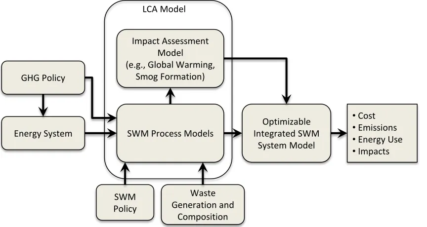
infrastructure is often in operation for decades, it is essential that integrated SWM models provide useful insights into how such changes may affect SWM. The generalized modeling framework for this research is shown in Figure 1-1.
Figure 1-1 Generalized modeling framework showing how energy system modeling is connected to LCA models for a SWM system, and how the outputs of these models are then used as inputs into an optimizable
LCA framework to systematically analyze future SWM.
The research goal will be met through the following research objectives:
1) Develop a generalized mathematical programming model capable of identifying SWM strategies that minimize cost or environmental impacts subject to other policy constraints (Chapter 2);
2) Use the optimization model to analyze the economic and environmental impacts and trade-offs associated with SWM strategies that consider future changes to waste generation, waste composition, and energy projections (Chapter 3); and
3) Analyze how variations in the energy system, GHG policy, and SWM policy affect optimal SWM decisions (Chapter 4).
Energy System
Optimizable Integrated SWM
System Model
•Cost •Emissions •Energy Use •Impacts Impact Assessment
Model
(e.g., Global Warming, Smog Formation)
LCA Model
GHG Policy
SWM Process Models
Waste Generation and
Composition SWM
4
2
A MULTISTAGE OPTIMIZATION MODEL FOR LIFE-CYCLE
ASSESSMENT-BASED INTEGRATED SOLID WASTE
MANAGEMENT
2.1 Introduction
Solid waste management (SWM) is an integral component of civil infrastructure and the broader U.S. economy. In 2010, U.S. municipal solid waste (MSW) systems processed approximately 250 million tons of waste. The direct emissions from landfilling, composting, and combustion of waste resulted in an estimated 123 Tg of CO2e emissions, representing over 10% of non-energy related greenhouse gas (GHG) emissions. Landfills, which received 54% of MSW in 2010, are currently estimated to be the third largest source of anthropogenic methane in the U.S. (U.S. EPA, 2011 and U.S. EPA, 2012). MSW also contains significant quantities of recoverable materials and can be used for energy recovery, making the SWM system a highly visible and potentially high-impact target for enhancing environmental sustainability. Expected future GHG mitigation policies are likely to impact the cost and strategic direction of SWM. Given the complexity of SWM, even subtle changes to SWM programs pose potential for unintended environmental consequences. The appropriate selection of waste processing technologies and efficient waste management strategies offer opportunities to minimize environmental impacts, particularly through energy and materials recovery. An effective SWM strategy must account for the complex interdependencies and interactions among waste handling processes (e.g., collection, material recovery, biological and thermal treatment, and landfilling) and their effects on competing management
objectives (e.g., minimize cost, maximize net energy production, increase waste diversion from landfills, and minimize GHG emissions). The framework presented here is intended to optimize integrated SWM decisions at the solid waste system level (e.g., municipality or county), but the results of these system level analyses could be aggregated to analyze larger jurisdictions (e.g., state, provincial, regional, or national).
Life-cycle assessment (LCA) is a useful tool for systematically estimating the
Several LCA models have been developed to determine the environmental impacts associated with SWM systems (e.g., Dalemo et al., 1997; McDougall et al., 2001; Haight, 2004; Kirkeby et al., 2006). These models estimate the environmental impacts of various waste management alternatives, and can be used to perform “what-if” scenario analyses to quantify the environmental effects of incremental changes to the integrated system. While these models are an essential foundation that enables a systematic integrated analysis of SWM systems, they cannot simultaneously consider all possible waste collection and treatment alternatives to find the combination of technologies that optimizes environmental and economic objectives.
Only limited research in LCA-based optimization of integrated SWM has been reported (e.g., Harrison et al., 2001; Solano et al., 2002; Shmelev and Powell, 2006; and Hung et al., 2007). Previous research has generally focused on single-stage analyses that assume static systems, although real-world SWM strategies must adapt to population and policy changes as well as changes to waste generation and composition. While some previous research efforts have considered stage-wise decision-making in SWM (e.g., Li et al., 2006; Li and Huang, 2007; and Tan, 2010), they focused on relatively simple systems (e.g., a single or limited number of waste materials, a limited number of waste collection alternatives, little or no waste separation) without consideration of full life cycle emissions, and involved computationally demanding solution procedures (e.g., fuzzy quadratic programming , interval-parameter stochastic integer programming, inexact dynamic programming containing fuzzy boundary intervals). These approaches work well for small illustrative systems, but are not readily generalizable and scalable to larger systems.
Prior work has not addressed changes in energy infrastructure in response to evolving environmental policy and technological innovation that may affect the performance of SWM. Changes in the broader energy system due to changes in the national and regional electricity generation mix will affect the prices of fuel and electricity used in SWM as well as the emissions associated with electricity use. For example, replacing coal-fired electricity generation with natural gas or renewables will change the emissions associated with
6 integrated SWM models provide useful insights into how such changes affect SWM. Long-term changes to the energy system, which involve the slow turnover of long-lived capacity, motivate the development of a multi-stage optimization of SWM.
While prior models are useful, a general modeling framework is needed to more realistically represent actual SWM management systems, which include dozens of waste streams, varying generation sector types, dozens of potential collection and treatment processes, and multiple time stages. This paper presents the Solid Waste Optimization Life Cycle Framework (SWOLF), which is suitable for stage-wise decision support under different scenarios. SWOLF is capable of developing integrated SWM strategies that consider existing as well as new SWM infrastructure. This is a major advantage since the reduced incremental costs associated with continued use of existing infrastructure is often an important factor in long-term capital decision making. Section 2.2 describes the modeling framework and includes an illustrative example that demonstrates the capability of the framework to represent complex SWM systems. Section 2.3 describes a simple test system, which is used to help illustrate the mathematical description of the optimization model in Section 2.4. Section 2.5 presents a simple, illustrative analysis using the test system
described in Section 2.3, and Section 2.6 draws conclusions from the model formulation and application.
2.2 Integrated Solid Waste Management Modeling Framework
2.2.1 Life cycle assessment framework for solid waste management
Figure 2-1. Inputs and outputs for a generic waste treatment process model. Input masses and all outputs are specified per unit mass of each waste material. Model parameters and user inputs are used to characterize the transformation of the incoming waste mass as well as the resulting emissions, fuel use, and costs. User inputs represent the model parameters that are system-specific, which need to be specified by users, while default
values are available for other model parameters. 1 Mg = 1 metric ton.
Default model parameters are provided, but can also be changed by the user. For example, each piece of equipment in a material recovery facility (MRF) has a separation efficiency in units of Mg separated/Mgin and an electricity use coefficient in units of kWh/Mgin. Based on the incoming waste composition as well as the input and parameter values, each process model calculates the masses of output waste materials, emissions, fuel use, electricity use, capital costs, and operating costs. Emission factors have been developed for the emissions associated with equipment fuel use, transportation, chemical and biological transformations, and electricity use in each process. Life cycle impact factors can then be used with the life cycle inventory results to calculate environmental impacts from the emissions (e.g., global
Generic Process Model
Physically Separated Materials (e.g., recyclables, residuals)
(Mgout/Mgin)
Direct Emissions (kg/Mgin)
Equipment Fuel Use (L/Mgin)
Electricity Use (kWh/Mgin)
Capital Cost ($/Mginyr-1)
Operating Cost ($/ Mgin)
Incoming Waste Materials (Mgin)
User Inputs Model Parameters Biologically/Chemically Transformed Materials (e.g., ash, compost)
(Mgout/Mgin)
Stored Mass (Mgstored/Mgin)
8 warming potential, acidification potential, or human toxicity). To build an LCA model for an entire waste system, the mass flows from the appropriate combination of these unit processes are linked from waste collection through final disposal or beneficial recovery of material. Detailed documentation of the solid waste unit process models will be published elsewhere.
2.2.2 Mass flow modeling
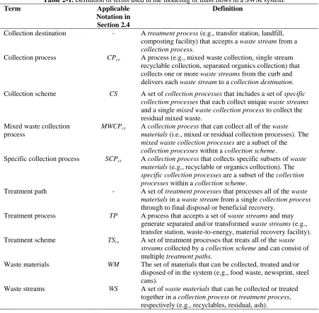
Table 2-1. Definition of terms used in the modeling of mass flows in a SWM system.
Term Applicable Notation in Section 2.4
Definition
Collection destination - A treatment process (e.g., transfer station, landfill, composting facility) that accepts a waste stream from a
collection process.
Collection process CPcs A process (e.g., mixed waste collection, single stream
recyclable collection, separated organics collection) that collects one or more waste streams from the curb and delivers each waste stream to a collection destination.
Collection scheme CS A set of collection processes that includes a set of specific collection processes that each collect unique waste streams
and a single mixed waste collection process to collect the residual mixed waste.
Mixed waste collection process
MWCPcs A collection process that can collect all of the waste materials (i.e., mixed or residual collection processes). The
mixed waste collection processes are a subset of the
collection processes within a collection scheme.
Specific collection process SCPcs A collection process that collects specific subsets of waste materials (e.g., recyclable or organics collection). The
specific collection processes are a subset of the collection processes within a collection scheme.
Treatment path - A set of treatment processes that processes all of the waste materials in a waste stream from a single collection process
through to final disposal or beneficial recovery. Treatment process TP A process that accepts a set of waste streams and may
generate separated and/or transformed waste streams (e.g., transfer station, waste-to-energy, material recovery facility). Treatment scheme TScs A set of treatment processes that treats all of the waste
streams collected by a collection scheme and can consist of multiple treatment paths.
Waste materials WM The set of materials that can be collected, treated and/or disposed of in the system (e.g., food waste, newsprint, steel cans).
Waste streams WS A set of waste materials that can be collected or treated together in a collection process or treatment process, respectively (e.g., recyclables, residual, ash).
10 bottles. The unique responses of each waste material to each process require that the mass flow of each individual waste material through the system be considered. This is challenging for a network flow model because all of the waste materials enter the system as a mixed entity, which reflects the waste composition of the generated mixed waste. For example, if one were to consider the use of a landfill and a waste-to-energy (WTE) facility, the optimal solution from a simple network model could send combustibles to the WTE facility, and the rest of the waste to the landfill, but the individual waste materials cannot be separated without the use of a dedicated separation facility. To ensure that waste materials are not inappropriately separated in a process, linked ratio constraints that introduce nonlinear expressions would have to be enforced for each waste material and process. This would result in a non-linear optimization model. Since the purpose of the model is to derive a readily scalable and generalizable framework, mass is balanced with only linear expressions using collection and treatment schemes that account for all mass flows from collection through treatment and final disposal or beneficial recovery.
Collection schemes collect all of the generated waste materials and consist of a
combination of collection processes (e.g., mixed waste collection + single stream recyclable collection + source separated organics collection) as well as the destination (e.g., landfill, material recovery facility, and composting) for each collection process. Valid collection schemes must include a way to collect all of the generated waste materials. For example, single stream recyclable collection combined with source separated organics collection do not make a valid collection scheme; a mixed waste collection process must be included to collect the non-recyclable and non-source separated organic waste materials. There are also limits on the proportion of each waste material that can be collected by each collection process. For example, only recyclable waste materials can be collected by recyclable
The mass of waste collected by each collection scheme must then be treated. The possible ways for collected waste to be treated are called treatment schemes, which vary for each
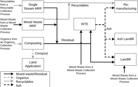
collection scheme. An example system that contains numerous potential treatment schemes is shown in Figure 2-2. Each collected waste stream must have an associated treatment path
that begins at a collection destination (i.e., single stream MRF, mixed waste MRF, composting, WTE, and landfill in this example) and ends in final disposal or beneficial recovery (i.e., remanufacturing or land application). The system shown in Figure 2-2 includes three collected waste streams (i.e., mixed waste, single stream recyclables, and organics).
Figure 2-2. An example of a set of treatment schemes that shows the potential waste flows for all of the collected waste. The organics and recyclable collection processes are both specific collection processes. The single stream MRF, mixed waste MRF, composting, WTE, and landfill are all potential collection destinations. In this example system, there are 102 possible treatment schemes and each one belongs to at least one collection
scheme. Single Stream MRF Mixed Waste MRF Composting Land Application WTE Re-manufacturing Landfill Ash Landfill Ash Residual Recyclables
Mixed Waste from a Mixed Waste Collection
Process Mixed Waste from a
Mixed Waste Collection Process Mixed Waste
12 Each of these waste streams has associated treatment paths that are shown in Figure 2-3. Even though only three waste streams are collected, reconfigured waste streams are
produced by the treatment processes (e.g., separated recyclables, compost, ash, and residual waste). The fraction of each waste material entering each treatment process that goes to each output waste stream is determined by both the treatment process and treatment scheme. For example, a representative treatment path consists of single-stream recyclables going to a single stream MRF, the separated recyclables from the single stream MRF going to remanufacturing, the MRF residual going to a WTE facility, and the ash from the WTE facility going to a landfill. In that example, a mixed recyclable waste stream is collected, but the MRF produces a separated recyclable waste stream, and a residual waste stream. The WTE facility then produces an ash waste stream when the residual waste stream is
combusted. The fraction of each waste material separated out in the single stream MRF is determined by the specified separation efficiency of the equipment used in the MRF. Similarly, the ash produced by each waste material entering the WTE facility is determined by the WTE process model based on the ash content of each waste material and the
combustion efficiency of the WTE facility. The treatment scheme determines the entire material flow from collection destination for each collection process in the associated
collection scheme through final disposal or beneficial use. In the example shown in Figure 2-2, a treatment scheme would consist of at least one mixed waste treatment path and at most one treatment path for each of the other waste streams (i.e., no more than one path from commingled recyclables and no more than one path from organics can be added to the chosen mixed waste path). This ensures that any treatment scheme uniquely and fully defines how all of the incoming waste is treated.
Figure 2-3. All the treatment paths for the example shown in Figure 2-2. Treatment schemes are produced by combining one mixed waste treatment path with at most one of each of the recyclable and source separated
organics paths (i.e., more than one of either is not allowed).
2.2.3 Facility capacity modeling
Given the long-lived nature of most SWM processes, it is necessary to consider changes in the SWM system, including the capital investments to build, expand, or replace facilities. Facility capacity can be updated in each stage, and the mass flow through a treatment process
is limited by the available facility capacity in each stage. The model can consider both existing and new facilities. The ability to include existing facilities allows the model to consider the lower costs often associated with existing infrastructure when determining the optimal solution. Facilities are constrained to a minimum feasible capacity specific to its process type (e.g., composting facilities can be built with smaller throughput capacity than
WTE LandfillAsh Landfill Mixed Waste MRF ReMfg Landfill WTE Landfill Mixed Waste MRF WTE Ash Landfill Mixed Waste MRF ReMfg WTE Landfill Single Stream MRF ReMfg WTE Ash Landfill Single Stream MRF ReMfg Landfill Single Stream MRF ReMfg Landfill WTE ReMfg WTE Landfill Composting Land Application Landfill Composting Land Application
Different Treatment Paths for Mixed Waste
Different Treatment Paths for Recyclables
Different Treatment Paths for Source Separated Organics
WTE Ash
Landfill Composting
14 WTE facilities). Each facility type has a lifetime over which it is active; and when its lifetime ends, its capacity is no longer available to treat waste. During the lifetime of the facility, the capacity of that facility can be expanded. If a facility is expanded, it must be expanded by at least a specified minimum expansion level that considers economies of scale. It is assumed that during expansion the necessary maintenance and repairs are performed to reset the facility life to its original lifetime. To maintain the new level of available capacity, the existing capacity is replaced by the expanded capacity. If the lifetime of a facility extends past the decision horizon, it is assumed to be rebuilt indefinitely at the end of its life to provide equivalent service beyond the decision horizon. This is consistent with other infrastructure planning studies, which assume that equivalent capacity exists indefinitely to meet the continuing service demand. If a facility becomes inactive before the end of the decision horizon, it can be decommissioned. The capacity decisions require the use of binary variables, resulting in a mixed integer linear programming (MILP) modeling framework to find the optimal integrated SWM plan.
2.2.4 Cost modeling
As with all civil infrastructure projects, it is necessary to consider both capital and operating costs. The costs associated with each unit process are provided by the life-cycle process model as shown in Figure 2-1. The capital costs for each process are reported in units of dollars per annual throughput capacity (i.e., $/Mg-yr-1, 1 Mg = 1 metric ton). Capital costs are generally defined as one-time construction-related costs. Capital costs are associated with building new facilities and expanding facilities in each stage as well as indefinitely
rebuilding capacity after the model time horizon for those facilities with active capacity at the end of the decision horizon. Capital costs used to build existing facilities are considered sunk and therefore do not affect future decisions.
based on their total consumption for processing each waste material as well as the fuel and electricity prices in each stage. Separating out the fuel and electricity costs allows the model to consider future changes in prices based on different energy and environmental policy futures.
Remanufacturing, collection, and landfills do not have an explicitly modeled capacity or capital costs (all capital costs are amortized into the operating costs). Remanufacturing covers a diverse array of facilities across a number of industries. The total capacity is
essentially infinite when compared to MSW recyclable generation, so remanufacturing costs and emissions are considered on a per unit mass recycled basis. The main capital expenditure for a collection process is the vehicles. The lifetime of collection vehicles is relatively short and the existence of resale markets for such vehicles makes it reasonable to incorporate their upfront cost into the operating costs. Since landfills are essentially continuing construction projects, it is difficult to reasonably differentiate capital and operating costs, and since landfill disposal is readily available in most locations for a flat fee per ton, the lack of capital decisions should not alter optimal solutions found by the model. Landfill lifetimes are also variable based on their utilization, so all landfill construction costs are amortized into their operating costs. Landfills can have cumulative capacity constraints that prohibit the model from disposing of more waste than an individual landfill can hold.
2.2.5 Environmental emissions modeling
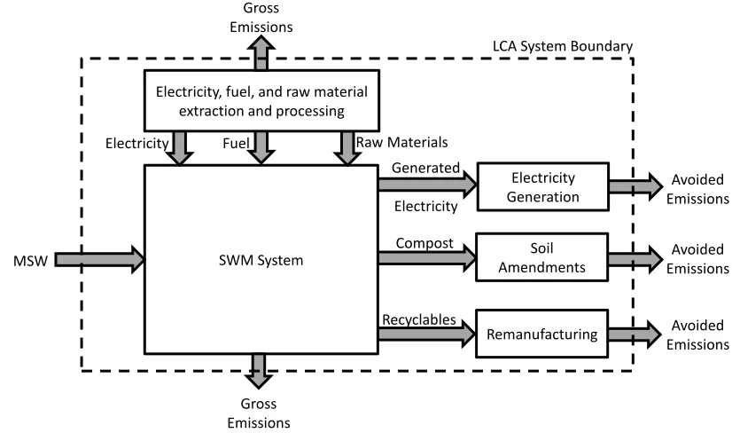
Figure 2-4 shows the system boundary for the LCA. All emissions are calculated for each
Figure 2-4. System boundary for the SWM life-cycle assessment. Gross emissions are generated through electricity, fuel, and raw material extraction and processing, as well as directly in SWM processes. Emission
offsets are produced from avoiding electricity generation, soil amendment production, and virgin material production. Net emissions are equal to the difference between gross and avoided emissions.
2.2.6 Solid waste management policy requirements
User-specified constraints can be added to analyze and explore specific SWM policies. A common consideration for solid waste decision-makers is the need to achieve diversion targets, which require that a specified percentage of waste mass not be disposed in landfills. The purpose of diversion targets is to encourage recycling and/or energy recovery of wastes, which ostensibly increase environmental sustainability. Users can also ban specific materials from entering particular process types. For example, many countries, states, and provinces have bans on sending various degradable waste materials to landfills. Such a policy would be modeled by setting the mass of those materials entering a landfill to zero. To eliminate a treatment process from consideration, either due to a regulatory ban or user preference, the treatment facility capacity can be set to zero. It is also possible to set economic (i.e., budget) constraints while minimizing environmental emissions or maximizing diversion. Users can
Generated
Electricity
SWM System Fuel
Electricity Raw Materials
Electricity Generation Remanufacturing Compost Recyclables Gross Emissions Avoided Emissions Avoided Emissions Avoided Emissions MSW
Electricity, fuel, and raw material extraction and processing
Gross Emissions
LCA System Boundary
18 also specify minimum utilization constraints for certain processes; these constraints ensure that if a facility is built, a minimum specified fraction of its capacity is utilized. For example, such a constraint applies to WTE plants that typically require at least 80% utilization for the plant to operate efficiently.
2.3 Illustrative Integrated Solid Waste Management System
The modeling framework outlined in Section 2.2 and explained with applicable mathematical expressions in Section 2.4 is generic and flexible. Here a specific illustrative example system (Figure 2-5) is used, without loss of generality, to help describe the model structure and the implementation of the mathematical programming model presented in Section 2.4. In this example, the waste is generated in each of the three, 10-year stages (Table 2-2).
Table 2-2. Waste generation for the illustrative SWM system shown in Figure 2-5. Generated Waste (Mg)
2010-2019 2020-2029 2030-2039
Recyclables 25,000 33,000 45,000
Non-recyclables 25,000 27,000 30,000
Figure 2-5. System model of potential mass flows for the illustrative example. WTE, LF, and MRF are all potential collection destinations. The residual waste collection process collects the waste mass not collected by recyclable collection. Recyclable collection requires residual waste collection to form a valid collection scheme.
The model parameter values used to generate the illustrative results can be found in Appendix A. The WTE facility is required to receive at least 80% of its capacity in each stage that it is active.
The illustrative example shown in Figure 2-5 includes two waste materials, namely, recyclables (Rec) and non-recyclables (NRec). These materials can be handled by three
collection processes: mixed waste collection (MWC), commingled recyclable collection (CRC), and residual waste collection (RWC). The RWC process collects the residual waste mass not collected by recyclable collection. The commingled recyclable collection process can collect at most 60% of the generated recyclables due to inconsistent recyclable separation by the waste generators. The possible collection destinations for mixed and residual waste are the landfill (LF) and WTE facility treatment processes. The only available destination for CRC is the MRF. The illustrative example includes an existing MRF (MRF_E) that has 10 years of remaining life with a capacity of 10,000 Mg/yr in operation during the first stage. A new MRF (MRF_N) can be built in any stage. The MRF_N has an assumed separation efficiency of 90%, compared to 80% for the MRF_E. Recovered recyclables from either MRF are sent to a remanufacturing (ReMfg) process. Residual from either MRF can be
20 disposed in the landfill or the WTE facility. Ash from WTE combustion can be disposed in a dedicated ash landfill (ALF) or a mixed waste landfill. Five percent of the incoming mass to the WTE facility is assumed to exit as ash.
The three collection processes are combined to form six collection schemes: 1) all
generated waste is collected as mixed waste and disposed at the landfill (MWC to LF); 2) all generated waste is collected as mixed waste and processed at the WTE facility (MWC to WTE); 3-4) recyclables are collected as commingled recyclables and the residual waste is collected separately and disposed in the landfill (CRC to MRF_E or MRF_N; and RWC to LF); and 5-6) recyclables are collected as commingled recyclables and the residual waste is collected separately and processed at the WTE facility (CRC to MRF_E or MRF_N; and MWC to LF). Each of the collection schemes also has associated treatment schemes that are shown in Table 2-3. In this illustrative example, treatment schemes are defined by where MRF residuals are treated, and where WTE ash is disposed. The mixed or residual waste
collection destination is determined by the collection scheme.
Table 2-3. Collection schemes and their associated treatment schemes in the illustrative example. The treatment scheme designations are formed from the destinations of mixed waste collection, MRF residuals, and ash. The illustrative system has three collection processes with six collection schemes, as well as 17 treatment schemes
(the number of collection andtreatment schemes that include a MRF are doubled to include the MRF_N and MRF_E alternatives).a
Collection Scheme Treatment Schemes Treatment Scheme Designationb Mixed Waste Destination MRF Residual Destination Ash Destination
MWC to LF L-- {LF }
MWC to WTE W-A {WTE ALF}
W-L {WTE LF}
CRC to MRF_N or MRF_E and RWC to LF
LL- {LF LF }
LWA {LF WTE ALF}
LWL {LF WTE LF}
CRC to MRF_N or MRF_E and RWC to WTE
WLA {WTE LF ALF}
WLL {WTE LF LF}
WWA {WTE WTE ALF}
WWL {WTE WTE LF}
a.MWC – Mixed waste collection, CRC – Commingled Recyclable Collection, RWC – Residual Waste
Collection, ALF – Ash Landfill, LF – Landfill, MRF_N – New MRF, MRF_E – Existing MRF, WTE – Waste-to-Energy
b.
2.4 Mathematical Expressions for the Integrated Solid Waste Management Model
A comprehensive set of expressions is required to appropriately model the SWM system. One set of constraints is used to ensure mass balance in each stage. Another set of constraints is used to assign each facility’s available capacity in each stage based on decisions made in preceding stages. Another set of expressions is used to calculate costs and other
environmental emissions. Finally, user-defined constraints can be added to meet other
objectives (e.g., diversion constraints, utilization constraints). The subsections below provide the mathematical model formulation, and the nomenclature used in the equations is included in the Symbols Used section.
2.4.1 Mass flow expressions
Mass flow constraints ensure that mass is conserved through each process and that waste composition only changes when a treatment process alters the composition through physical, chemical, or biological means (e.g., MRFs separate recyclables from non-recyclables, WTE combusts waste and produces ash, composting facilities convert organics to compost). The mass flow constraints for a single stage were developed based on the modeling approach described by Solano et al., (2002), which has been generalized and extended in this paper to accommodate multiple stages. Based on our functional unit of waste at curbside, Eq. 1 ensures that all of the generated waste in each stage is collected by one of the collection schemes in each stage. In the illustrative example, FTP = 3, and CS = {{(MWC-LF)}, {(MWC-WTE)}, {(RWC-LF), (CRC-MRF)}, {(RWC-WTE), (CRC-MRF)}}.
∑
Eq. 1
Eq. 2 ensures that all of the waste collected by each collection scheme in a stage is assigned to an appropriate treatment scheme in that stage. The treatment schemes are indexed by
22 ∑
Eq. 2
Eq. 3 allocates the entire generated, collected, and treated waste mass to individual waste materials. In the illustrative example, WM = {Rec, NRec} and the composition of the generated mass found in Table 2-2 is used to calculate wm,tfor each material in each stage.
Eq. 3
Eq. 4 ensures that all of the collected and treated waste is allocated to a collection process.
The collection processes are indexed by the collection schemes to which they belong. In the illustrative example, CP mwc-lf and CP mwc-wte = {MWC}; and CP rwc-lf and CP rwc-wte = {CRC,
RWC}.
∑
Eq. 4
While Eq. 4 is used to ensure that the waste mass of each material is collected by a collection process, Eq. 5 ensures that waste materials are not collected at a proportion greater than the proportion at which they can be separated in a given specific collection process. For waste materials that cannot be collected by a given collection process, the maximum collection efficiency is zero (e.g., the maximum collection efficiency for NRec in CRC is zero). In the illustrative example, SCP mwc-lf and SCP mwc-wte = {Ø}; and SCP rwc-lf and SCP rwc-wte =
{CRC}.
Eq. 5
While Eq. 5 defines the maximum mass of each waste material that can be collected by each
collection processes is collected in a mixed waste collection process. In the illustrative example, MWCPmwc-lf and MWCPmwc-wte = {MWC}; MWCPrwc-lf and MWCPrwc-wte =
{RWC}.
∑
Eq. 6
Eq. 5 and Eq. 6 define the mass of each waste material collected through each collection process and treatment scheme, and Eq. 7 is used to define the total mass of each waste material collected via each collection process by summing over every treatment scheme
associated with the collection scheme to which the collection process belongs.
∑
Eq. 7
Eq. 8 is used to determine the mass of each waste material delivered from each collection process to each treatment process. In the illustrative system WTE, MRF, and landfill are the
treatment processes that accept waste from collection, and are thus the collection destinations.
∑ ∑
Eq. 8
Eq. 9 and Eq. 10 are used in conjunction with Eq. 8 to determine the mass of each waste material processed through each treatment process in each treatment scheme. Eq. 9 defines the output mass of each waste material in each waste stream from each treatment process in each treatment scheme. In the illustrative system, WS = {Ash, Recyclables, Residual}. Eq. 10 defines the incoming mass of each waste material into each treatment process in each
24
destination through to final disposal and/or beneficial recovery is determined by the
treatment scheme and the characteristics of the treatment processes in that treatment scheme.
∑
Eq. 9
∑ ∑
Eq. 10
Eq. 11 sums the incoming mass of each waste material through each treatment process in each treatment scheme to determine the total mass of each waste material processed through each treatment process in each stage, so that operating costs and process emissions can be assigned to each treatment process and waste material in each stage.
∑
Eq. 11
2.4.2 Facility capacity expressions
The preceding mass flow equations are used to ensure that all of the waste mass is collected and treated in every stage, but they do not provide any constraints on what capacity is available to treat the waste. Eq. 12 is used to ensure that the total mass of waste processed through each capital treatment process in each stage does not exceed the available capacity for that treatment process. In the illustrative example, CAP = {MRF_E, MRF_N, WTE}.
∑