ABSTRACT
HARTIS, BRETT MICHAEL. Mapping, Monitoring and Modeling Submersed Aquatic Vegetation Species and Communities. (Under the direction of Stacy A. C. Nelson).
Aquatic macrophyte communities are critically important habitat species in aquatic systems worldwide. None are more important than those found beneath the water’s surface,
commonly referred to as submersed aquatic vegetation (SAV). Although vital to such systems, many native submersed plants have shown near irreversible declines in recent decades as water quality impairment, habitat destruction, and encroachment by invasive species have increased. In the past, aquatic plant science has emphasized the restoration and protection of native species and the management of invasive species. Comparatively little emphasis has been directed toward adequately mapping and monitoring these resources to track their viability over time. Modeling the potential intrusion of certain invasive plant species has also been given little attention, likely because aquatic systems in general can be difficult to assess. In recent years, scientists and resource managers alike have begun paying more attention to mapping SAV communities and to address the spread of invasive species across various regions. This research attempts to provide new, cutting-edge techniques to improve SAV mapping and monitoring efforts in coastal regions, at both community and individual species levels, while also providing insights about the establishment potential of
Mapping, Monitoring and Modeling Submersed Aquatic Vegetation Species and Communities
by
Brett Michael Hartis
A dissertation submitted to the Graduate Faculty of North Carolina State University
in partial fulfillment of the requirements for the Degree of
Doctor of Philosophy
Fisheries, Wildlife, and Conservation Biology
Raleigh, North Carolina 2013
APPROVED BY:
_______________________________ _______________________________
Stacy A.C. Nelson Robert J. Richardson
Chair of Advisory Committee
_______________________________ _______________________________
ii
DEDICATION
iii
BIOGRAPHY
Brett Hartis was born and raised in Marion, North Carolina the son of Gary and Brenda Hartis. His love for all things outdoors began at a young age and was greatly fostered
by his family. Brett found interests in fishing and hunting throughout the beautiful Blue Ridge Mountains of Western North Carolina. After graduating high school in the top of his class, Brett headed east to East Carolina University and quickly began studying the estuarine and marine systems of coastal NC. After having the opportunity to do research with various
experts in the field of fisheries science, Brett graduated from the ECU with a 4.0 and an award for outstanding senior in the Department of Biology. He then moved to Raleigh, North Carolina to pursue further interests in natural resources and geographic information
systems, obtaining a Master of Science degree in Fisheries, Wildlife, and Conservation Biology and North Carolina State University.
iv
ACKNOWLEDGEMENTS
I would like to thank my committee, my chair Dr. Stacy Nelson, and members Dr. Rob Richardson, Dr. Heather Cheshire and Dr. JoAnn Burkholder for their continued guidance and support in obtaining this seemingly life-long goal. Dr. Nelson has supported and guided me throughout my graduate degrees providing both professional and personal guidance. Dr.
Richardson gave me the amazing opportunity to work in extension providing me with a wealth of knowledge and support in aquatic plant management. Dr. Cheshire has given
excellent guidance in the study of GIS and remote sensing as well as giving me the opportunity to teach on multiple occasions and Dr. Burkholder has opened my eyes to a wide
v
TABLE OF CONTENTS
LIST OF TABLES ...ix
LIST OF FIGURES ...xi
CHAPTER 1 Introduction ...1
1.1 Mapping, Monitoring and Modeling Submersed Aquatic Vegetation ...1
1.2 Primary Research Questions and Rationale ...5
1.3 References ...8
CHAPTER 2 Plants and Pixels: Developing Predictive Models of Submersed Aquatic Vegetation Using Satellite Imagery in the Currituck Sound, North Carolina USA ...12
2.1 Introduction ...12
2.2 Materials and Methods ...15
2.2.1 Study Area ...15
2.2.2 SAV Sampling ...16
2.2.3 Water Quality Characteristics ...18
2.2.4 Satellite Imagery ...19
2.2.5 Statistical Analysis ...21
2.2.6 LOGIT Model Calibration ...24
2.2.7 Accuracy Assessment of LOGIT Models ...25
2.3 Results ...26
2.3.1. SAV Cover in Currituck Sound ...26
2.3.2 LOGIT Model results ...27
2.3.2.1 Worldview-2 ...28
2.3.2.2 Quickbird ...29
2.3.2.3 LANDSAT5 ...30
vi
2.3.3. Accuracy Assessment of Models ...30
2.4. Discussion ...31
2.5. References ...37
CHAPTER 3 A Novel Technique for Mapping of Submersed Aquatic Vegetation Species Dominance and Coverage in Mixed Stands of Large, Shallow Coastal Systems ...57
3.1. Introduction ...57
3.2. Materials and Methods ...61
3.2.1. Study Area ...61
3.2.2. SAV Field Sampling ...62
3.2.3. Geostatistical Analysis ...64
3.2.4. Interpolation: Inverse Distance Weighted ...65
3.2.5. Development of a Dominance/ Percent Cover Metric ...66
3.3. Results ...67
3.3.1 SAV Survey Results ...67
3.3.2. Species Heterogeneity and Coverage ...67
3.3.3 Geostatistical Results ...68
3.3.4. Maps of DOMCOV by Species ...68
3.4. Discussion ...69
3.5. Conclusions ...72
3.6. References ...74
CHAPTER 4 Modeling the Establishment Potential of Hydrilla (H. verticillata) in North America ...89
4.1. Introduction ...89
vii
4.2.1. Data Sources ...93
4.2.2. Risk Scale Development ...94
4.2.3. State/ Province Risk Assessment ...96
4.2.4. Risk Based on Water Body Size ...97
4.3. Results ...98
4.3.1. Risk Scale ...98
4.3.2. State/ Province Risk Assessment ...98
4.3.3. Risk Based on Water Body Size ...99
4.4. Discussion ...100
4.5. Conclusions ...102
4.6. References ...106
CHAPTER 5 Conclusions ...116
5.1. Conclusions ...116
5.2. Chapter 2: Does remote sending provide a viable alternative to traditional survey techniques of SAV in shallow, coastal systems? ...116
5.3. Chapter 3: Do spatial interpolations offer an accurate picture of SAV species and community dynamics? ...117
5.4. Chapters 2 and 3: Implications for impairment of SAV in the Currituck Sound ...118
5.5. Chapter 4: Does H. verticllata really have the potential to become invasive across the northern ranges of North America? ...121
5.6. References ...122
APPENDICES ...124
Appendix A – Chapter 2 Supplement ...125
viii
ix
LIST OF TABLES
Table 2.1. Sensor specifications for spatial, spectral, radiometric and temporal resolution ...41 Table 2.2. Multi-Spectral bands of the WorldVeiw-2 satellite sensor ...42 Table 2.3. Multi-Spectral bands of the Quickbird satellite sensor ...43 Table 2.4. Summary statistics of all water quality and condition parameters collected during summer field sampling ...44 Table 2.5. Percent concordant value for each presence/absence model developed ...45 Table 2.6. Analysis of Maximum Likelihood estimates for the Worldview-2 sensor
specific model applied to the August 5th, 2010 dataset ...46 Table 2.7. Parameter estimates for the Worldview-2 sensor specific model applied to the July 22nd, 2010 dataset ...47 Table 2.8. Parameter estimates for the best Worldview-2 image specific model applied to the August 5th, 2010 dataset ...48 Table 2.9. Analysis of Maximum Likelihood estimates for the Quickbird sensor
specific model applied to the September 13th, 2010 dataset ...49 Table 2.10. Worldview-2 accuracy assessments for both sensor and image specific
Models...50 Table 2.11. Quickbird accuracy assessments for sensor specific model ...51
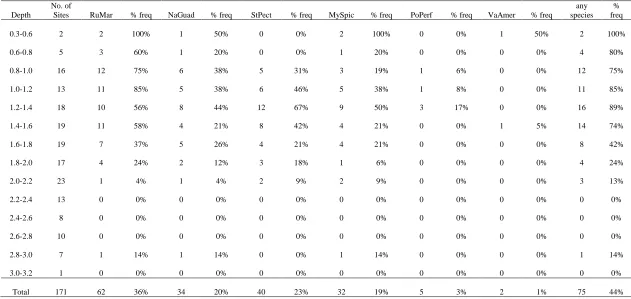
Table 3.1. Plant frequency-depth relationships for Currituck Sound study area ...77 Table 3.2. Average values (Min and Max) by species for SAVDOM, TOTSPEC and
x
Table 4.1. Summary statistics of all U.S. states/ Canadian provinces analyzed in model development ...109 Table 4.2. Mean establishment risk of states/ provinces falling along the maximum risk gradient and mean establishment risk between water bodies within states/provinces ...110 Table 4.3. Type III test of mixed effects for state and size class ...111
Table B.1. Correlation matrix of SAV across species ...136 Table B.2. Sediment type distribution of the littoral zone and number of vegetated points in each ...137
xi
LIST OF FIGURES
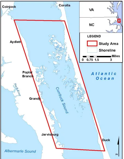
Figure 2.1. Study area for SAV sampling and remote sensing within the Currituck Sound making up the uppermost portion of the Albemarle-Pamlico Estuary System ...52 Figure 2.2. The distribution of plant cover levels throughout the Currituck Sound ...53 Figure 2.3. Worldview-2 sensor specific model predictions applied to image taken on August 5th, 2010 and overlain with SAV percent cover estimations from survey 2 ...54 Figure 2.4. Worldview-2 image specific model predictions applied to image taken on 08/05/10 and overlain with SAV percent cover predictions from survey 2 ...55 Figure 2.5. Quickbird sensor specific model predictions applied to image taken on July 13th, 2010 and overlain with SAV percent cover predictions from SAV survey 2 ...56
Figure 3.1. Study area for SAV sampling ...80 Figure 3.2. Derived depth contours of each SAV species based on field observations ...81 Figure 3.3. Example SAVHET output displaying spatial heterogeneity of M. spicatum
throughout the study area ...82 Figure 3.4. DOMCOV output displaying estimated coverage distribution of M. spicatum
throughout the study area ...83 Figure 3.5. DOMCOV output displaying estimated coverage distribution of N.
guadalupensis throughout the study area ...84 Figure 3.6. DOMCOV output displaying estimated coverage distribution of P. perfoliatus
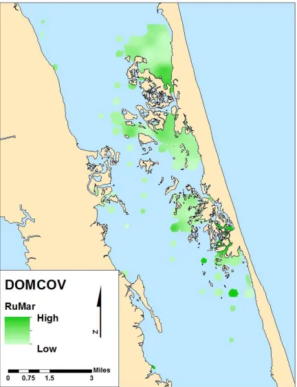
throughout the study area ...85 Figure 3.7. DOMCOV output displaying estimated coverage distribution of R. maritima
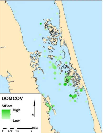
throughout the study area ...86 Figure 3.8. DOMCOV output displaying estimated coverage distribution of S. pectinata
throughout the study area ...87 Figure 3.9. DOMCOV output displaying estimated coverage distribution of V. americana
xii
Figure 4.1. Average minimum monthly temperature (June, July and August) of
H. verticillata occurrences ...112
Figure 4.2. Potential H. verticillata establishment based on average of all growing season months. ...113
Figure 4.3. Risk scale of H. verticillata and linear regression of minimum (low occurrence, low temperature) and maximum (high occurrence, first peak) risk ...114
Figure 4.4. Model representation of H. verticillata establishment potential in the United States and Canada ...115
Figure A.1. SAV presence/ absence and percent change over time in Currituck Sound ...118
Figure A.2. Total waterfowl population estimates within the Currituck Sound (as adapted from Baker and Valentine 2007) ...119
Figure A.3. Image acquisition area ...120
Figure A.4. Littoral zone defined for remote sensing purposes ...121
Figure A.5. Worlview-2 image acquired on 07/22/10 ...122
Figure A.6. Worldview-2 Image acquired on 08/05/10 ...123
Figure A.7. Quickbird image acquired on 09/13/10 ...124
Figure A.8. LANDSAT5 images acquired on multiple dates ...125
Figure A.9. SAV presence/ absence run 1 ...126
Figure A.10. SAV presence/ absence run 2 ...127
Figure A.11. Worldview-2 sensor specific model overlain with SAV percent cover ...128
Figure A.12. Worldview-2 image specific model overlain with SAV percent cover ...129
Figure A.13. Quickbird image specific model overlain with SAV percent cover ...130
Figure A.14. Depth gradient along defined littoral zone ...131
xiii
Figure A.16. Quickbird derived model overlain with original image ...133
Figure A.17. Secchi depth averaging across entire study area ...134
Figure A.18. Total nitrogen profile across study area ...135
Figure B.1. Distribution of soil type throughout the study area as estimated during SAV sampling ...138
Figure B.2. Species as a percentage of all vegetated points as estimated using Sincock et al. 1965 ...139
Figure B.3. Species as a percentage of all vegetated points as estimated in this study ...140
Figure C.1. Hydrilla occurrence worldwide as designated by master dataset ...142
Figure C.2. United States and Canada water bodies ...143
Figure C.3. Hydrilla establishment potential by water body ...144
Figure C.4. Projected establishment potential model +1 degree C ...145
Figure C.5. Projected establishment potential model +3 degree C ...146
1
CHAPTER 1
Introduction
1.1 Mapping, Monitoring and Modeling Submersed Aquatic Vegetation
Aquatic systems are as mysterious as they are complex. Unlike terrestrial systems, the monitoring, management and assessment of such environments is greatly hindered by
limitations of humans, as organisms foreign to life in aquatic habitats. Extensive monitoring protocols, management handbooks, and assessment manuals have been written for many terrestrial ecosystems. By comparison, the aqueous domain of planet Earth is poorly understood.
Some aspects of aquatic systems, such as the biotic and physical realms, have seen standardization of protocols and methodologies for monitoring and assessment over the past few decades. However, one of the most important aquatic communities in need of
understanding still lacks widely accepted methodologies that can provide consistently precise and accurate measures (Systma 2008). Aquatic vascular plant populations found in various water bodies worldwide, while critically important habitat species, generally have been “beyond reach” except for relatively primitive methods for monitoring and assessment.
2
reproduce beneath the water’s surface. Submersed aquatic vegetation (SAV) is a diverse group of vascular plants found in various climates throughout the world (Waycott et al 2009, Street et al. 2005). SAV provides food, shelter and critical habitat for many animal species (Larkum et al. 2006). The disappearance of native species or the introduction and dispersal of invasive species can cause severe ecological and economic impacts (Langeland 1996, Charles and Dukes 2007). Ecological impacts are centered on the fact that the entire food web dynamics can be significantly altered by the addition or removal of a single keystone or exotic species (Irlandi et al. 1995, Hovel and Lipcius 2002). Invasive submersed species, in particular, displace native plants and can shift balanced, heterogeneous ecosystems to monocultures with severely altered food web dynamics (Richardson et al. 2012). Invasive SAV can also promote lethal impacts affecting higher trophic levels. For example, an
3
thousands to millions of U.S. dollars (e.g. Larkum et al. 2006, Pimental et al. 2005, Costanza et al. 1997, Anderson 1993). Indirect economic losses, more difficult to define and
sometimes of major importance, only add to this deficit (Pimental et al. 2005). Thus, the methods by which to detect, monitor and assess SAV, including evaluation of the efficacy of management actions, have become increasingly important (Blossey 2004). Potentially as important as determining SAV species composition in a given water body can be determining the geographic extent of species distributions, confounded by climate change (Johnston 1986). This is especially the case with invasive species, which can cause great economic hardship and ecological damage in the wake of their expansion.
Various methodologies for detection and monitoring of SAV lack rigorous standardization and explicit protocols. Most commonly, these methods are employed to develop species lists, estimate plant abundance, and determine species distributions within a given water body (Madsen and Wersal 2012). Techniques for monitoring SAV range from low-cost, high-effort point-intercept sampling to high-cost, moderate-effort remote sensing, each of which can provide very different information. For example, point-intercept sampling provides the researcher with the presence or absence of various species, but without intensive sampling, information on the extent and distribution of plants is left to speculation or some degree of interpolation. Remote sensing can provide valuable distribution and extent
4
most applicable to a given project. The method that most meets the desired objectives of the study is used; no one-size-fits-all method can be fit across all systems (Spencer and
Whitehand 1993).
Detection and monitoring of SAV has become extremely important over the past few decades, especially as non-native species have continued to establish and spread throughout various water bodies in North America as throughout the world (Williams and Meffe 1998). Determining where a species presently exists in a water body is important, yet accurately estimating the extent to which a species may expand beyond its established range can be just as vital (Johnstone 1986). For example, accurate prediction of the potential establishment of an invasive SAV species can greatly aid resource managers in maximizing preventative and precautionary measures.
5
1.2Primary Research Questions and Rationale
Chapter 2: Large-scale submersed aquatic vegetation (SAV) surveys are rarely done due to logistical difficulties and high costs. This characterization especially fits the shallow, low- salinity, highly diverse coastal aquatic habitats of North Carolina. The primary reason for difficulty in obtaining survey data over large areas is largely due to the expense, intensive labor need and time constraints associated with sampling SAV. In past years, remote sensing coupled with modeling and interpolation techniques has shown the potential to be an
important tool to obtain survey information on SAV over large lakes across the country (Nelson et al. 2006, Valley et al., 2005). However, this approach has limited applicability for assessing SAV distributions in shallow, coastal regions where frequently changing, tidal and wind-driven currents cause high, persistent turbidity. Therefore, an approach that can address the need for regional-scale water body mapping and monitoring of SAV in these coastal areas would be valuable. Survey assessments are further complicated in coastal regions covering thousands of hectares. The second chapter of this dissertation examines whether remote sensing can be used to detect SAV presence and/or levels of cover in the Currituck Sound, a shallow, low-salinity water body on the northeastern coast of North Carolina.
6
nearly continual littoral coverage. In such systems, a method to identify key areas for further exploration and survey should be employed to help focus management efforts.
Understanding the dynamics of SAV populations in a given water body has become increasingly important, especially with the increasing encroachment of various invasive species that can severely alter community dynamics (Madsen and Wersal 2012).
Furthermore, assessing individual species dominance and coverage within large stands of vegetation provides the essential information needed to make sound decisions about optimal management strategies. Here, I developed a geographic information systems (GIS)-based and field driven mapping technique to identify the present spatial locations and coverage of SAV species in the Currituck Sound of North Carolina. The spatial distribution of the invasive species, Myriophyllum spicatum, was also targeted.
7
8
1.3. References
Ailstock, M. S., D. J. Shafer, and A. D. Magoun. 2010. Effects of planting depth, sediment grain size, and nutrients on Ruppia maritima and Potamogeton perfoliatus seedling
emergence and growth. Restoration Ecology 18: 574-583. DOI: 10.1111/j.1526-100X.2010.00697.x
Anderson LWJ. 1993. Aquatic weed problems and management in North America (a) Aquatic weed problems and management in the western United States and Canada. In: AH Pieterse and KJ Murphy (eds.), Aquatic Weeds. Oxford University Press, Oxford. pp. 371-391.
Bailey JE and Calhoun AJK. 2008. Comparison of three physical management techniques for controlling variable-leaf milfoil in maine lakes. J Aquat Plant Manage 46:163-7.
Balciunas J and Chen P. 1993. Distribution of hydrilla in northern china - implications on future spread in north-america. J Aquat Plant Manage 31:105-9.
Blossey B. 2004. Monitoring in weed biological control programs, pp. 95-105. In: EM Coombs, JK Clark, GL Piper and AF Cofrancesco, Jr. (eds.). Biological control of invasive plants in the United States. Oregon State University Press, Corvallis.
Brunel S. 2009. Pathway analysis: Aquatic plants imported in 10 EPPO countries. Bulletin OEPP 39(2):201-13.
Busch, K. E., R. R. Golden, T. A. Parham, L. P. Karrh, M. J. Lewandowski, and M. D. Naylor. 2010. Large-scale Zostera marina (eelgrass) restoration in Chesapeake Bay, Maryland, USA. Part I: A comparison of techniques and associated costs. Restoration Ecology 18: 490-500. DOI: 10.1111/j.1526-100X.2010.00690.x
Costanza R, R d’Arge, R de Groote, S Farber, M Grasso, B Hannon, K Limburg, S Naeem, RV O’Neill, J Paruelo, RG Raskin, P Sutton, and M van den Belt. 1997. The value of the world’s ecosystem services and natural capital. Nature 387:253-260.
Charles H and JS Dukes. 2007. Impacts of invasive species on ecosystem services. Biol Invas 193:217- 237
9
Gordon, D.R., 1998. Effects of Invasive, Non-indigenous plant species on ecosystem processes: Lessons from Florida. Ecological Applications. 8: 975-989.
Hovel KA, Lipcius RN (2002) Effects of seagrass habitat fragmentation on juvenile blue crab survival and abundance. J Exp Mar Biol Ecol 271:75–98
Irlandi EA, Ambrose WG Jr, Orlando BA (1995) Seascape ecology and the marine
environment: how spatial configu-ration of seagrass habitat influences growth and survival of the bay scallop. Oikos 72:307–313
Johnstone IM. 1986. Plant invasion windows: A time-based classification of invasion potential. Biological Reviews 61(4):369-94.
Klosowski S. 2006. The relationships between environmental factors and the submerged potametea associations in lakes of north-eastern poland. Hydrobiologia 560:15-29.
Langeland, K.A. 1996. Hydrilla verticillata (L.F.) Royle (Hydrocharitaceae), “The Perfect Aquatic Weed”. Castanea. 61(3): 293-304.
Larkum, A.W.D., Orth, R.J., Duarte, C., 2006. Seagrasses: Biology, Ecology and Conservation. Springer, The Netherlands. 691.
Madeira, P.T., C.C.Jacono, and T.K. Van. 2000. Monitoring hydrilla using two RAPD procedures and the nonindigenous aquatic species database. J. Aquat. Plant Manage. 38:33-40.
Madsen JD and JA Bloomfield. 1993. Aquatic vegetation quantification symposium: an overview. Lake and Reserv. Manage. 7:137-140.
Madsen JD and RM Wersal. 2012. A Review of Aquatic Plant Monitoring and Assessment Methods. Aquatic Ecosystem Restoration Foundation.
Middelboe AL and S Markager. 1997. Depth limits and minimum light requirements for freshwater macrophytes. Freshwater Bio. 37:553-568
10
Nichols C and Shaw B. 1986. Ecological life histories of the 3 aquatic nuisance plants, myriophyllum-spicatum, potamogeton-crispus and elodea-canadensis. Hydrobiologia 131(1):3-21.
Peterson A, Papes M, Kluza D. 2003. Predicting the potential invasive distributions of four alien plant species in north america. Weed Sci 51(6):863-8.
Pimentel D, R Zuniga and D Morrison. 2005. Update on the environmental and economic costs associated with alien-invasive species in the United States. Ecol. Econ. 52: 273-288. Richardson et al. 2012. Monoecious Hydrilla – A Review of the Literature. Northeast Aquatic Nuisance Species Panel. Accessed Online:
http://www.nyis.info/user_uploads/files/Monoecious%20Hydrilla%20Lit%20Review%20-%20Final.pdf
Spencer DF and LC Whitehand. 1993. Experimental design and analysis in field studies of aquatic vegetation. Lake and Reserv. Manage. 7:165-174.
Street, M.W., Deaton, A.S., Chappel, W.S., Mooreside, P.D., 2005. North Carolina Coastal Habitat Protection Plan, North Carolina Department of Environment and Natural Resources, Division of Marine Fisheries, Morehead City, NC. 656 pp. Online at
http://www.ncfisheries.net/habitat/chpp2k5/_Complete%20CHPP.pdf
Sytsma MD. 2008. Introduction: workshop on submersed aquatic plant research priorities. J. Aquat. Plant Manage. 46:1-7.
Valley, R.D., Drake, M.T., Anderson, C.S., 2005. Evaluation of alternative interpolation techniques for the mapping of remotely-sensed submersed vegetation abundance. Aquat. Bot. 81, 13–25.
Waycott, M., Duarte, C.M., Carruthers, T.J., Orth, R.J., Dennison, W.C., Olyarnik, S., Calladine, A., Fourqurean, J.W., Heck, K.L., Hughes, A.R., Kendrick, G.A., Kenworthy, W.J., Short, F.T, Williams, S.L., 2009. Accelerating loss of seagrasses across the globe threatens coastal ecosystems. Proceedings of the National Academy of Sciences 106, 12377-12381.
11
Williams, S.K., J. Kempton, S.B. Wilde, and A. Lewitus. 2007. A novel epiphytic
cyanobacterium associated with reservoirs affected by avian vacuolar myelinopathy. Harmful Algae. 6:343–353.
Williams, J.D.; G. K. Meffe (1998). "Nonindigenous Species". Status and Trends of the Nation's Biological Resources. Reston, Virginia: United States Department of the Interior, Geological Survey 1.
Wilson CJ, Wilson PS, Greene CA, Dunton KH. 2013. Seagrass meadows provide an acoustic refuge for estuarine fish. Mar Ecol Prog Ser 472:117-27.
12
CHAPTER 2
Plants and Pixels: Developing Predictive Models of Submersed Aquatic Vegetation using Satellite Imagery in the Currituck Sound, North Carolina USA
2.1 Introduction
Large-scale submersed aquatic vegetation (SAV) surveys are rarely possible, although effective SAV management depends in part on understanding the coverage and spatial location of SAV. The primary reason for such difficulty in obtaining survey data over large areas is largely due to the expense, intensive labor need and time constraints associated with sampling SAV. Survey assessments are further complicated in coastal regions covering thousands of hectares. SAV plays an extremely important role ecologically, providing critical habitat for fish, shellfish, and other wildlife as well as supporting local fisheries based economies (Larkum et al. 2006). The most extensive SAV communities in North Carolina tend to be found in shallow, low-salinity waters on the leeward side of the state’s barrier island network (Davis and Brinson 1983, Ferguson and Wood 1994, Street et al. 2005). Inventorying an area this large becomes cost-, time-, and labor-prohibitive using traditional field sampling techniques such as visual delineation, sampling along transects, or
13
Remote sensing using modeling and interpolation techniques have exhibited the potential to be an important tool to obtain survey information on SAV cover in large lakes (Nelson et al. 2006, Valley et al. 2005). The utility of remote sensing to measure SAV has been demonstrated through the process of mapping general SAV distributions through visually driven delineations (Orth and Moore, 1983; Marshall and Lee, 1994), including North Carolina’s coastal waters (Ferguson and Korfmacher 1997). Remote sensing has been successfully applied to assess SAV in clear tropical waters worldwide (Chollett and Mumby 2012, Dierssen et al. 2010, Lyzenga et al. 2006). However, this approach has limited applicability for assessing SAV distributions in shallow, coastal regions where frequently changing, wind-driven currents yield high, persistent turbidity. Therefore, it would be valuable to design an approach that could be used for large-scale water body mapping and monitoring of SAV in these turbid coastal areas.
14
absorption of light in the water column. Additionally, turbid water often contains
appreciable suspended sediment and other constituents that also scatter or absorb light. As a result, researchers typically have used remotely sensed data to detect emergent or floating vegetation, rather than SAV (see Baschuk et al. 2012, Albright and Ode 2011, Midwood and Chow-Frasier 2010). Improvements in spatial resolution are providing greater differentiation in the sample scene, whereas advancements in spectral resolution may make it possible to discern spectral properties of submersed plants that previously could not be identified. Water characteristics and quality may also need to be taken into consideration when attempting to remotely sense SAV. For decades remotely sensed images have been used to measure characteristics such as chlorophyll, water depth, Secchi depth transparency, and suspended sediment concentrations (Nelson et al. 2003, Khorram and Cheshire 1985), all of which may influence SAV detection. Coastal waters like the Currituck Sound can vary widely in several of these water quality characteristics, which in turn can influence how well aquatic SAV can be characterized with remote sensing. Characteristics such as turbidity and water depth may influence the sensor’s ability to detect SAV, making it necessary to
15
The objectives in this study were: (1) to determine whether different levels of aquatic plant cover could be detected using the commercially available Quickbird and Worldview-2 satellite sensors or free LANDSAT 5 data and (2) to assess whether predictions of SAV abundance and distribution can be improved by considering environmental characteristics (Secchi disk depth, salinity, sediment type, and water depth) and water quality (total nitrogen, total phosphorus, etc) in the models.
2.2 Materials and Methods 2.2.1 Study area
16
through shallow water channels. Inputs of brackish water from federal canals also might influence the salinity of Currituck Sound. The sound is separated from the Atlantic Ocean by a narrow strip of barrier islands known as the outer banks which are no more than a mile wide. Unlike many other sounds which are tidally driven, water level fluctuations in Currituck Sound are a product of the constantly changing wind. Thus, water level can fluctuate wildly from week to week, even from day to day during changing weather conditions. The Sound stretches through two counties, Dare and Currituck, with level or slightly sloping terrain.
The SAV survey area spans the mid portion of the Currituck Sound encompassing the Currituck County mainland and Outer Banks as well as the Dare County Outer Banks (Figure 1). The study area is approximately 21 km long by 8 km wide, stretching from just south of the towns of Corolla and Duck, NC on the eastern side and Parker’s creek to Webster’s creek on the western side.
2.2.2. SAV sampling
17
removed as SAV would be unable to establish growth on such features. Therefore, only points in the littoral zone of the Sound remained for survey 2 (N = 117). Survey 3 consisted of 41 points within the littoral zone area. All survey points were located in the field using a Magellan Mobile Mapper CX professional grade GPS unit with sub-meter positional accuracy. At each point, water depth was measured to sediment using a marked depth pole, and plant metrics were assessed by recording plant presence and plant cover at each site. This was accomplished by assigning an associated level of plant coverage for each category. Plant cover was assessed at each point for an area of 10 m x 10 m by using a two-sided sampling rake thrown in four cardinal directions from the point of anchor. A two-sided rake is a widely accepted survey method for assessing plant presence/absence, wherein the rake is thrown and drug along the bottom to retrieve plant material (Madsen 1999). A locational error of +/- 1.52 m was estimated through frequent repositioning.
18
detect different levels of SAV coverage, a littoral percent plant cover was calculated as the total number of points sampled with any plant category greater than level 0 (i.e., >1% cover at an individual site), divided by the total number of points in the littoral zone. These values were used to estimate the applicability of using literature defined thresholds for each sensor. In turbid North Carolina coastal bodies of water, SAV is unable to typically establish or grow in depths greater than 1.83 m due to inadequate light (Ferguson and Korfmacher 1997, Kenworthy and Haunert 1991). Thus, areas greater than 2 m in depth were deemed “pelagic.”
2.2.3. Water Quality Characteristics
19
For water quality estimations, a representative dataset was developed from which to test water quality. This representative dataset was then interpolated to provide water quality at each SAV sample point. Water quality parameters identified below were tested between SAV sampling runs: Water Quality sampling 1 (July 8th, 2010 – July 23rd, 2010) and Water Quality sampling 2 (August 8th, 2010 – August 14th, 2010). Water quality parameters were estimated with the use of a field spectrophotometer. Measures of water quality included total nitrogen (TN), total phosphorus (TP), ammonia nitrogen, nitrate-N, color, dissolved oxygen (DO), nitrite-N, Phosphate-P, and pH. DO, pH, and color were all derived in the field using procedures designated for testing by LaMotte (2000). All other samples were collected into 950 ml sampling containers, preserved using procedures specified by LaMotte (2000), transported to the lab in complete darkness, packed in ice, and processed the same day as collection.
2.2.4. Satellite imagery
20
1 pixel per transformation. All imagery was inspected for atmospheric differences occurring between scenes and histogram matching was completed when necessary. Due to the high occurrence of clouds in most images, a cloud removal masking technique was required to remove all pixels containing clouds or cloud shadows. All land features were masked out using similar techniques. Data points lying within pixels containing clouds, shadows or other interference were subsequently removed from the dataset before statistical analyses were performed. Dark object subtraction was used in an attempt to adjust for further atmospheric correction (Teillet and Fedosejevs 1995).
The spectral pixel values or digital number (DN) values for all single pixels
containing the position of each sample point, using the field-recorded GPS coordinates, were extracted using ESRI ArcMap 10.0 (ESRI 2011). Digital Number values were extracted from each individual scene and combined with all SAV sampling data into one database file. Spectral DN values for the pelagic region were also extracted to analyze the relationship between pelagic zone sound characteristics and spectral values. Because the pelagic zone is more homogeneous than the littoral zone, the spectral DN values for all pixels within the pelagic zone of the aggregated sampling areas were averaged resulting in one pelagic spectral value. Spectral and spatial properties of each sensor used are included in Tables 1, 2, and 3.
Because of the high spatial resolution of the Worldview-2 and Quickbird sensors, it was necessary to resample pixel size to more closely match the resolution of SAV survey sites (10m X 10m). Resampling was achieved using a bilinear interpolation in ESRI ArcMap 10.0 (ESRI 2011). LANDSAT 5 DN extraction was based solely on the single pixel
21
resolution (30m) than both Worldview-2 and Quickbird. 2.2.5. Statistical analysis
Survey point extractions were analyzed for outliers and determination of outliers was completed using visual and statistical inspection of each DN value at each point. Any DN value identified as an outlier (> 1.5 x IQR) in SAS Enterprise Guide 4.2 (SAS 2009) was ultimately inspected for atmospheric interference and removed upon confirmation. Points removed were deemed unusable in model development due to the high degree of influence from sources outside of the target. This procedure was completed for each image/ SAV sampling dataset combination. All spectral digital number values were independently and statistically evaluated for interference from atmospheric or sensor defects before attempting to develop a spectral model data set for each sensor.
The satellite imagery DN values and SAV data were analyzed using binomial and multinomial logistic regression (logit models) in SAS Enterprise Guide 4.2 (SAS 2009). Stepwise and best-subset regression techniques were used to fit individual and combined spectral bands to the sample data.
22
For binomial logistic regression, the logit model indicated how the explanatory variable (DN values by band) affects the probability of the event (SAV presence/absence) being observed versus not being observed. For the multinomial logistic regression, probable outcomes of observations were calculated by analyzing a series of binomial sub models that represented the overall ability of the model to predict each of the plant cover response variables. For all logit model analyses, the descending option was used to select the highest plant category level as the response variable reference (level 3 for plant cover and level 1 for littoral plant presence/absence). This selection ensured that the results will be based on the probabilities of modeling an event (SAV present), rather than a non-event (SAV not present).
Model fit was determined by examining the percent concordant values, the Wald test statistic, likelihood ratio, and score test. The percent concordant values provided an
indication of overall model quality through the association of predicted probabilities and observed responses. These values were based on the maximum likelihood estimation of the percent of paired observations of which values differed from the response variable
23
on predicted probabilities, and then computes a chi-square from observed and expected frequencies (Hosmer and Lemeshow 2000). Then a probability (p) value is computed from the chi-square distribution with 8 degrees of freedom to test the fit of the logistic model. If the Hosmer and Lemeshow Goodness-of-Fit test statistic is 0.05 or less, the null hypothesis is accepted that there is no difference between the observed and model-predicted values of the dependent. (This means the model predicts values significantly different from observed values.) If the Hosmer and Lemeshow Goodness-of-Fit test statistic is greater than 0.05, then the null hypothesis cannot be rejected - there is no difference, implying that the model's estimates fit the data at an acceptable level.
24
Logit models for individual images were used to examine whether various water quality characteristics helped improve predictions of SAV cover using Quickbird, Worldview-2 and LANDSAT 5 imagery. Ordinary least squares regression was used to regress each of the model coefficients from the individual image logit models against each of the measured water quality characteristics individually: Secchi depth, water depth, salinity, water temperature, sediment type, TN, TP, NH4+N, nitrate-N, color, DO, nitrite-N,
Phosphate-P, and pH.
2.2.6 LOGIT Model Calibration
25
2.2.7. Accuracy Assessment of LOGIT models
Typical measures of error in models are “omission” and “commission” errors. These
measures are most often used to determine how well a model corresponds with groundtruthed data at the same location. For this study, we compared rake sample results to the sensor derived LOGIT models as an additional means for evaluating model results. We used two classes to develop error estimates of correspondence between field and sensor derived
presence/absence category data: ‘SAV’ (for indication of SAV presence) or ‘no SAV’ (for no
indication of SAV presence). We used four classes to develop error estimates of
correspondence between field and sensor derived percent cover category data: ‘No Cover’ (for indication of <20% coverage), ‘Low Cover’ (for indication of 21-40% coverage), ‘Medium Cover’ (for indication of 41-80% coverage) and ‘High Cover’ (for 81-100%
coverage).
26
2.3. Results
2.3.1. SAV cover in the Currituck Sound
The average Secchi depth in the study area was 0.42 m throughout the sample period. Water quality and other environmental conditions are summarized in Table 4. During
summer sampling, SAV was found to be present on average at 47% of all points sampled, and the majority of all points (53%) were devoid of plants. Although nearly half of all points sampled were vegetated, only 22% of the SAV was in classes designated as “detectable” through remote sensing (> 20% coverage). Almost half of all vegetated points fell below this 20% threshold (24%). The category 1 level (21-40%) comprised 11% of all vegetated points, while levels 2 (41-80%) and 3 (81-100%) represented 8% and 3% of all vegetated points, respectively (Figure 2). Thus, SAV distribution within the Currituck Sound exhibited a highly patchy distribution which further complicated detection with remote sensing. Six SAV species were identified during summer sampling, including five native species as
Ruppia maritima (widgeon grass), Najas guadalupensis (southern naiad), Stuckenia pectinata
27
2.3.2. LOGIT Model Results
Sensor-derived logistical regression models were developed for SAV presence or absence. However, no models could be developed for the multinomial variable (plant cover) due to a low ratio of events to non-events. In the case of the multinomial variable (plant cover), an event was defined as any plant cover category 1-3 which indicated some type of SAV presence. A non-event was defined as the plant cover category 0 which indicated no plant presence. The automated stepwise selection method led to the final, most reasonable model as decided upon in the best-subset procedure for the regression analysis. For a variable to enter into or remain in the model, a p-value of < 0.01 was necessary. A model was considered fit if the Hosmer and Lemeshow Goodness-of-Fit test yielded an insignificant difference in groups (p > 0.05). Sensor specific models were developed for both the
Quickbird and Worldview-2 sensors, but LANDSAT 5 models proved to be inconclusive. Odds ratios were used to evaluate relative influence of variables selected in the final models. Prediction maps were developed to display 3 categories: correct prediction (prediction = observation), false positives (prediction = 1, observation = 0), or false negatives (prediction = 0, observation = 1).
Several environmental characteristics were highly correlated with SAV
presence/absence, but only Secchi depth and water depth improved actual model predictions. Worldview-2 derived models yielded the highest percent concordant value for correct
28 2.3.2.1 Worldview-2
LOGIT model results suggested that the Worldview-2 sensor provided the best
predictive model of the binary predictor variable (presence/absence), with percent concordant values between 67.9 and 94.7% and Wald, Likelihood and Score values of < 0.0001 each. Three variables were included in the Worldview-2 sensor specific prediction model (Table 6). The most influential predictor variable for the Worldview-2 sensor-specific model was the interaction between band 4 and Secchi depth, followed by the interaction between band 3 and Secchi depth, band 4 alone and band 3 alone. The negative β coefficient for band 4 alone
was consistent with knowledge of the reflective properties of submersed plants in wavelengths from 700 to 1100 nm (Klancik et al. 2012). The negative β coefficient associated with the interaction of band 3 and Secchi depth was consistent with both the reflective properties of plants in wavelengths from 600 to 700 nm and the fact that light penetration decreases as Secchi depth increases. The positive associations with band 3 alone and the interaction between band 4 and Secchi depth were also consistent with reflective properties of plants. Regarding the best image provided for the Worldview-2 sensor (August 5th, 2010), model outputs demonstrated only 4 false negatives (observation dataset =
presence, prediction dataset = absence) and 3 false positives (observation dataset = absence, prediction dataset = presence).
29
This image-specific model suggested that only the interaction between band 4 and Secchi depth was the best predictor for the model. This image-specific model yielded a percent concordant value of between 88.5% and 94.7% and a Wald, Likelihood and Score values of <0.001. The positive β coefficient association with the interaction between band 4 and
Secchi depth was consistent with knowledge of the reflective properties of SAV from 700 to 1100 nm.
Parameter estimates for each Worldview-2 model are included in Table 7 for the sensor- specific model and in Table 8 for the image-specific model. Prediction output examples for the proposed Worldview-2 sensor derived model and the image-specific model (August 5th, 2010 dataset) are shown in Figure 3 and Figure 4, respectively. For comparison of prediction output to actual groundtruth estimates, SAV percent cover was overlain for each image/model combination.
2.3.2.2. Quickbird
The Quickbird sensor-derived predictive model yielded a percent concordant value of 73.1% with a Wald of 0.04, Score of 0.0097 and a Likelihood ratio of 0.0175. The most influential predictor variable was band 3 alone, followed by the interaction of band 2 and Secchi depth, band 3 and Secchi depth, band 2 alone, and a small influence provided by the interaction between band 4 and depth. The positive β coefficient for band 3 alone was
30
600 nm. The positive β coefficient for the interaction between band 2 and Secchi depth was consistent with knowledge of the reflective properties of submersed plants in wavelengths from 520 to 600 nm and the fact that light penetration decreases as Secchi depth increases. The negative β coefficient associated with the interaction of band 3 and Secchi depth was
consistent with both the reflective properties of plants in wavelengths from 600 to 700 nm and the fact that light penetration decreases as Secchi depth increases. Lastly, the negative β coefficient associated with the interaction of band 4 and depth was consistent with
knowledge of submersed plant reflection in wavelengths from 700 to 1000 nm and the fact that light penetration decreases as depth increases. Parameter estimates for the Quickbird-derived model are included in Table 9. The sensor-specific model prediction output for the Quickbird sensor is shown in Figure 5.
2.3.2.3. LANDSAT5
The LANDSAT-5-derived models yielded inconsistent results, often varying from scene to scene, and suggested various bands that have not historically been associated with plant reflectance. Although various images were available for analysis, many were affected by clouds, atmospheric haze, and sun-glint.
2.3.3. Accuracy Assessment of Models
31
4. Discussion
Remote sensing in Currituck Sound provides some potential for inventorying the distribution of SAV, but a number of limitations still exist and will be discussed in the following section. Overall, the Worldview-2 sensor provided the best predictive model of SAV presence or absence. A percent concordant value greater than 80% has been loosely recognized as an indicator of strong model agreement when developing predictive models that analyze the presence of SAV (Nelson et al 2006).
Models derived from the Worldview-2 sensor produced higher predictive capacity based on the groundtruthed field data in the Sound. Image and sensor specific models when applied to the August 5th, 2010 image provided percent concordant values of 81.3 to 91.6%. However, accuracy assessments of both the sensor specific and image specific Worldview-2 models showed relatively large commission and omission errors. False positives using the Worldview-2 derived models, although few, most often occurred in areas of shallow depth (<0.9 m) and could have been caused by bottom reflectance. However, four out of the seven false positives that occurred across all images with the Worldview-2 sensor took place at points with at least some SAV present (1-20%). The > 20% coverage threshold used to develop our models designated these points as “absent” of SAV, because these data points
32
image appeared very pixilated, having been acquired on a day of high wind and wave action. False negatives most often occurred in areas of low to moderate plant density (< 40%) or in areas of deeper water (> 0.9 m). Perhaps spectral contribution of SAV was inhibited by greater distances between plant canopy and water surface or high turbidity. Lower densities of SAV may also not provide an adequate spectral contribution to be differentiated from the water column alone. Patchy distributions of SAV, common in Currituck Sound, may also have contributed to false negatives. For example, SAV coverage in the survey area may not have covered an adequate amount of each pixel area for detection.
The Quickbird sensor provided poor results with a total of 10 false negatives and 1 false positive, and a percent concordant value of 73.1%. Unfortunately, one of the difficulties encountered with development of the Quickbird model was the lag time between image acquisition and field sampling (+ 36 days). This lag time prevented acquisition of near-coincidental satellite and field sampling, which may have contributed to limitations in model development; there were also large amounts of cloud cover in the Quickbird image. Most false negatives in the image were located along a large cloud extending from the southern to northern reach of the study area. Atmospheric interference inherent around clouds can severely alter the spectral signature of the target (Levin and Levina 2007), thus leaving even points not directly within the cloud at risk for atmospheric influences.
33
within individual pixels. Pixels likely contained plant matter but were potentially subject to complicated optical effects in very shallow waters, i.e. substratum reflectance contributed to tainted spectral reflectance. Several bands not historically associated with plant reflectance were potentially important, but were inconsistent. For example, band 5 and 7 (SWIR1 and SWIR2) were often identified as important. Given that these wavelengths do not penetrate water (Poole and Atkins 1926), these observations may have been related to spectral mixing of land or emergent vegetation features not sampled within the images large pixel size (30mx30m).
Although three models were developed, common variables emerged from each Worldview-2 model as well as the Quickbird Model - Band 4 and Secchi Depth. These two predictor variables were used in each model and should be investigated first in future attempts at remote sensing of SAV with the Worldview-2 sensor. The reflective properties of plants in the Near-Infrared portion of the electromagnetic spectrum have been cited in numerous papers regarding aquatic plants (e.g. Klancnik 2012, Nelson 2006), but water readily absorbs light in the NIR. This most likely limits the effective depth of Band 4 in most sensors to less than 1m in depth. Remote sensing of SAV using the NIR band, in this case, most likely detects plant material at shallow sites that are very close to the water surface.
34
made it possible to more adequately capture the sample area from which the groundtruth data were based. This became the major limitation to using freely available LANDSAT 5 data. The sensors 30-m spatial resolution most likely allowed spectral contribution from sources other than the target SAV (i.e. water-column constituents, turbidity, bottom reflectance, etc.). Although LANDSAT 5 imagery have been used in past attempts to remote sense SAV, the patchy distribution of SAV in Currituck Sound is likely the reason for the sensor’s poorer performance in this attempt to apply it for remote sensing of SAV presence/absence.
Complications arose using all sensors due to the low occurrence of events to non-events in the groundtruthed data making it difficult to satisfy general assumptions for applying logit models. Logistic regressions are improved when features of interest, in this case SAV presence, constitute a third of the total number of sample sites (Harrell 1997). Development of predictive models was for SAV presence, as this feature (“event”)
35
Difficulties in image acquisition from commercial vendors led to less-than-ideal available acquisition dates. Originally, images were scheduled to be acquired as close temporally to the actual dates of field surveys as possible. Inability to do so especially applied to the Quickbird image acquired in mid-September, leaving Surveys 1 and 2
36
37
2.5. References
Albright, T.P., and Ode, D.J., 2011. Monitoring the Dynamics of an Invasive Emergent Macrophyte Community using Operational Remote Sensing Data. Hydrobiologia 661.1, 469-74.
Baschuk, M.S., Ervin, M.D.,Clark, W.R., Armstrong, L.M., Wrubleski, D.A., Goldsborough, G.L.. 2012. Using Satellite Imagery to Assess Macrophyte Response to Water-Level
Manipulations in the Saskatchewan River Delta, Manitoba. Wetlands 32.6, 1091-102. Biber, P.D., Paerl, H.W., Gallegos, C.L., Kenworthy, W.J., Fonseca, M.S. 2004. Evaluating Indicators of Seagrass Stress to Light. in SA Bortone (ed.), Estuarine Indicators. CRC Press, Boca Raton. 193-209.
Burkholder JM, Tomasko DA, Touchette BW. 2007. Seagrasses and eutrophication. J Exp Mar Biol Ecol 350(1-2):46-72.
Chollett I and Mumby PJ. Predicting the distribution of montastraea reefs using wave exposure. Coral Reefs. 2012 JUN;31(2):493-503.
Curran, R.W. 2011. The Utility of Digital Globe’s WorldView‐2 Satellite Data
in Mapping Seagrass in North Carolina Estuaries. Unpublished results. Master’s Thesis, East Carolina University.
Davis, G.J.; and M.M. Brinson. 1983. Trends in submerged macrophyte communities of the Currituck Sound: 1909-1979. Journal of Aquatic Plant Management 21, 83-87.
Dierssen HM, Zimmerman RC, Drake LA, Burdige D. Benthic ecology from space: Optics and net primary production in seagrass and benthic algae across the great bahama bank. Mar Ecol Prog Ser. 2010;411:1-15.
Dogan, O.K., Akyurek, Z., and Beklioglu, M. 2009. Identification and Mapping of Submerged Plants in a Shallow Lake using Quickbird Satellite Data. Journal of environmental management 90.7, 2138-43.
Ferguson, R.L., Korfmacher, K. 1997. Remote sensing and GIS analysis of seagrass meadows in North Carolina, USA. Aquatic Botany. 28, 241-258.
Ferguson, R.L.; and L.L. Wood. 1994. Rooted vascular aquatic beds in the Albemarle-Pamlico estuarine system. NMFS, NOAA, Beaufort, NC, Project No. 94-02 , 103.
38
ESRI. 2011, ArcGIS Desktop: Release 10. Redlands, CA: Environmental Systems Research Institute.
Harrell, F. E. 1997. Predicting outcomes: applied survival analysis and logistic regression. University of Virginia Press. University of Virginia School Medicine, Charlottesville, Virginia.
Hosmer D.W. and Lemeshow S., 2000. Applied logistic regression, 2nd ed. New York: John Wiley &. Sons, Inc,. ISBN 0-471-35632-8.
Intergraph. 2010. ERDAS Imagine Desktop 2010. Madison, AL: Intergraph Geospatial. Khorram, S., Cheshire, H.M., 1985. Remote sensing of water quality in the Neuse River Estuary North Carolina. Photogramm. Eng. Remote Sens. 51, 329–341.
Klancnik, K., Mlinar, M., Gaberscik, A., 2012. Heterophylly Results in a Variety of "Spectral Signatures" in Aquatic Plant Species. Aquatic Botany. 98.1, 20-6.
Kleinbaum, D.G., 1994. Logistic Regression A Self-learning Text. Springer-Verlag Publishing, New York.
LamottE. 2000. LaMotte Smart Spectro Operator’s Manual. V3.0 and higher. 2000-01-MN Larkum, A.W.D., Orth, R.J., Duarte, C., 2006. Seagrasses: Biology, Ecology and
Conservation. Springer, The Netherlands. 691.
Lehmann, A., Jaquet, J.M., and Lachavanne, JB. 1997. A GIS Approach of Aquatic Plant Spatial Heterogeneity in Relation to Sediment and Depth Gradients, Lake Geneva, Switzerland. Aquatic Botany 58.3-4, 347-61.
Levin IM and Levina E. 2007. Effect of atmospheric interference and sensor noise in retrieval off optically active materials in the ocean by hyperspectral remote sensing. Appl Opt 46(28):6896-906.
Lyzenga DR, Malinas NR, Tanis FJ. Multispectral bathymetry using a simple physically based algorithm. IEEE Trans Geosci Remote Sens. 2006 AUG;44(8):2251-9.
Madsen, J.D., 1999. Point intercept and line intercept methods for aquatic plant management. Army Corps of Engineers Waterways Experiment Station Technical Note MI-02.
Marshall, T.R., Lee, P.F., 1994. Mapping aquatic macrophytes through digital image analysis of aerial photographs: assessment. J. Aquat. Plant Manage. 32, 61–66.
39
Midwood, J.D., and Chow-Fraser, P. 2010. Mapping Floating and Emergent Aquatic Vegetation in Coastal Wetlands of Eastern Georgian Bay, Lake Huron, Canada.Wetlands 30.6, 1141-52.
Nelson, S.A.C., Cheruvelil,K.S. and Soranno, P.A. 2006. Satellite Remote Sensing of Freshwater Macrophytes and the Influence of Water Clarity. Aquatic Botany 85.4, 289-98. Nelson, S.A.C., Soranno, P.A., Cheruvelil, K.S., Batzli, S.A., Skole, D.L., 2003. Regional assessment of lake water clarity using satellite remote sensing. J. Limnol. 62, (Suppl. 1), 27– 32.
Orth, R.J. Marion, S.R., Moore, K.A., Wilcox, D.J., 2010. Eelgrass (Zostera marina L.) in the Chesapeake Bay region of mid-Atlantic coast of the USA: challenges in conservation and restoration. Estuaries and Coasts 33, 139-150.
Orth, R.J., Moore, K.A., 1983. Submerged vascular plants: techniques for analyzing their distribution and abundance. Mar. Technol. Soc. 17, 38–52.
Pampel, F.C., 2000. Logistic Regression: A Primer. Sage University Papers Series
Quantitative Applications in the Social Sciences, series no. 07-132. Sage Publications, CA. Poole HH and Atkins WRG. 1926. On the penetration of light into sea water. Jour Marine Biol Assoc 14((1)):177-98.
SAS Institute Inc. 2009. Administering SAS Enterprise Guide 4.2. Cary, NC: SAS Institute Inc.
Sincock, J.L. 1965. Back Bay – Currituck Sound data report. U.S. Fish and Wildlife
Service, North Carolina Wildlife Resources Commission, and Virginia Commission of Game and Inland Fisheries. 1600.
Street, M.W., Deaton, A.S., Chappel, W.S., Mooreside, P.D., 2005. North Carolina Coastal Habitat Protection Plan, North Carolina Department of Environment and Natural Resources, Division of Marine Fisheries, Morehead City, NC. 656 pp. Online at
http://www.ncfisheries.net/habitat/chpp2k5/_Complete%20CHPP.pdf
Thayer, G.W., W.J. Kenworthy, Fonseca, M.S., 1984. The ecology of eelgrass meadows of the Atlantic coast: a community profile. U.S. Fish and Wildlife Service. FWS/OBS-84/02. 147.
40
Waycott, M., Duarte, C.M., Carruthers, T.J., Orth, R.J., Dennison, W.C., Olyarnik, S., Calladine, A., Fourqurean, J.W., Heck, K.L., Hughes, A.R., Kendrick, G.A., Kenworthy, W.J., Short, F.T, Williams, S.L., 2009. Accelerating loss of seagrasses across the globe threatens coastal ecosystems. Proceedings of the National Academy of Sciences 106, 12377-12381.
Valley, R.D., Drake, M.T., Anderson, C.S., 2005. Evaluation of alternative interpolation techniques for the mapping of remotely-sensed submersed vegetation abundance. Aquat. Bot. 81, 13–25.
41
Table 2.1. Sensor specifications for spatial, spectral, radiometric and temporal resolution.
Sensor Spatial (m)
Spectral (nm)
Radiometric (bits)
Temporal
(days) Bands
Worldview-2 1.8-2.4 450-1040 11 3.7 4*
Quickbird 2.44-2.88 450-900 11 3.5 4
LANDSAT-5 30 (120 Band 6) 450-1250 8 7 7
42
Table 2.2. Multi-Spectral bands of the WorldVeiw-2 satellite sensor
Worldview-2
Band 1 2 3 4
Name Blue Green Red NIR
Spectrum Width
(nm)
450 - 510
510 - 580
630 - 690
43
Table 2.3. Multi-Spectral bands of the Quickbird satellite sensor
Quickbird
Band 1 2 3 4
Name Blue Green Red NIR
Spectrum Width
(nm)
450 - 520
520 - 600
630 - 690
44
Table 2.4. Summary statistics of all water quality and condition parameters collected during summer field sampling.
Parameter mean (SD*) min max
depth (m)* 1.73 (0.602) 0.335 3.2
Secchi (m)* 0.42 (0.093) 0.2 0.75
temperature (oC) 29 (2.177) 22.22 32.33
Turbidity (NTU) 0.693 (0.541) 0.02 2
Ammonia-N (mg/L) 0.295 (0.094) 0.12 0.57
Color (cu) 327.28 (41.985) 184 405
DO (mg/L) 7.485 (0.934) 4.9 10.2
Nitrite-N (mg/L) 0.147 (0.042) 0.07 0.27
Nitrate-N (mg/L) 10.075 (1.664) 6 13
pH 7.378 (1.209) 5.7 9.2
Phosphate-P 0.015 (0.0163) 0 0.08
TN (mg/L) 1.075 (1.490) 0 8
TP (mg/L) 0.693 (0.541) 0.02 2
TN : TP 7.519 (19.353) 0 100
45
Table 2.5. Percent concordant value for each presence/absence model developed. *WVSS = Worldview-II Sensor Specific, WVIS = Worldview-II Image Specific, QB = Quickbird
Model
Percent Concordant
No. of Usable Points
WV SS 81.3 196
WV IS 91.6 80
46
Table 2.6. Analysis of Maximum Likelihood estimates for the Worldview-II sensor specific model applied to the August 5th, 2010 dataset.
Parameter DF Estimate SE Wald Pr > Chi Sq
Intercept 1 -2.2755 0.7678 8.7843 0.003
B3 1 0.5497 2.1038 0.0683 0.7939
B4 1 -4.9392 3.0326 2.6527 0.1034
B3*SD 1 -5.4005 4.6811 1.3309 0.2486
47
Table 2.7. Parameter estimates for the Worldview-II sensor specific model applied to the July 22nd, 2010 dataset.
Parameter DF Estimate SE Wald Pr > Chi Sq
Intercept 1 -1.8425 0.295 39.0086 < 0.0001
B3 1 19.1947 7.5488 6.4655 0.011
B4 1 -22.3063 7.8728 8.0278 0.0046
B3*SD 1 -46.3251 20.0271 5.3506 0.0207
48
Table 2.8. Parameter estimates for the best Worldview-II image specific model applied to the August 5th, 2010 dataset.
Parameter DF Estimate SE Wald Pr > Chi Sq
Intercept 1 -2 0.4859 16.94 < 0.0001
49
Table 2.9. Analysis of Maximum Likelihood estimates for the Quickbird sensor specific model applied to the September 13th, 2010 dataset.
Parameter DF Estimate SE Wald Pr > Chi Sq
Intercept 1 1.8684 0.3393 30.3157 <.0001
B2 1 -11.4288 5.4478 4.401 0.0359
B3 1 12.4367 5.373 5.3576 0.0206
B2*SD 1 31.7167 14.3848 4.8615 0.0275
B3*SD 1 -30.4846 14.0404 4.7141 0.0299
50
Table 2.10. Worldview-II accuracy assessments for both sensor and image specific models
Image (08/05/10) Specific Model
Omission LOGIT Model
SAV No SAV
Field Data SAV 31.3% 11 5
No SAV 4.7% 3 61
51
Table 2.11. Quickbird accuracy assessments for sensor specific model.
Sensor Specific Model
Omission LOGIT Model
SAV No SAV
Field Data SAV 62.5% 6 10
No SAV 1.4% 1 73
52
53
Figure 2.2. The distribution of plant cover levels throughout the Currituck Sound.
0% 20% 40% 60% 80% 100%
SAV Cover
0 (0-20%)
1 (21-40%)
2 (41-80%)
54
55
56
57
CHAPTER 3
A Novel Technique for Mapping Submersed Aquatic Vegetation Species Dominance and Coverage in Mixed Stands of Large, Shallow Coastal Systems
3.1. Introduction
In recent years, several agencies have developed strategies for protection of existing native submersed aquatic vegetation (SAV) communities through restoration of historical growth areas in large coastal systems (Ailstock et. al 2010, Busch et al. 2010). Along with restoration, efforts to control invasive species are often employed to help restore native populations (Gordon 1998). While various mapping and survey techniques are often employed to aid in these efforts, each has limitations for identifying key information about the spatial extent and coverage of SAV species in large project areas common of coastal systems. For example, aerial photography has commonly been used to address overall SAV coverage in large coastal systems (Orth et al. 2010, Orth et al. 2007, Niedier 2004), but in reality it is often seriously limited by water clarity and depth and does not provide critically needed, species-specific information. Likewise, boat based visual estimations have provided information on the localized extent of SAV but do not provide information on the species present (Madsen and Bloomfield 1993). As in aerial photography, visual estimations can also be confounded by water clarity (Yin and Kreiling 2011). Traditional sampling
58
techniques are exacerbated in coastal systems with a seemingly endless and dynamic littoral zone. In such systems, a method to identify key areas for further exploration and survey should be employed to help narrow down management efforts. Understanding the dynamics of SAV populations in a water body has become increasingly important, especially with the encroachment of various invasive species that can severely alter community dynamics (Madsen and Wersal 2012). Furthermore, assessing individual species dominance and coverage within large stands of vegetation provides the detrimental information needed to make sound decisions for what types of management should be employed. Historic studies have often reported species dominance on a system-wide basis (McAtee 1919, Kerwin et al 1976, Davis and Carey 1981) rather than expressing quantitative aspects of spatial
dominance within the study area. While informative in terms of presence/absence, such an approach provides no spatial reference to particular stand location or individual species dominance, heterogeneity or coverage which can be vital information when assessing plant communities. These features, particularly current species dominance and coverage, play a key role in efforts to restore and protect vital areas while monitoring the spatial location of invasive aquatic plant species (Lirman et al. 2008).
Assessment and identification of individual species dominance and coverage has been commonplace in terrestrial survey science for decades (Bechtold and Patterson 2005).