Formulation of a Vector SIS Malaria Model in a Patchy Environment with Two Age Classes

(1)

http://dx.doi.org/10.4236/am.2014.510147

How to cite this paper: Wairimu, J., et al. (2014) Formulation of a Vector SIS Malaria Model in a Patchy Environment with Two Age Classes. Applied Mathematics, 5, 1535-1545. http://dx.doi.org/10.4236/am.2014.510147

Formulation of a Vector SIS Malaria Model in

a Patchy Environment with Two Age Classes

Josephine Wairimu

1,2*

, Sallet Gauthier

2

, Wandera Ogana

1

1_{School of mathematics, University of Nairobi, Nairobi, Kenya} 2_{INRIA, Metz and University of Lorraine, Metz, France}

Email: *[email protected]

Received 6 March 2014; revised 6 April 2014; accepted 13 April 2014

This work is licensed under the Creative Commons Attribution International License (CC BY). http://creativecommons.org/licenses/by/4.0/

Abstract

We formulate an SIS model describing transmission of highland malaria in Western Kenya. The host population is classified as children, age 1- 5 years and adults, above 5 years. The susceptibili-ty and infectivisusceptibili-ty of an individual depend on age class and residence. The large scale system with 6n equations is reduced into a compact form of 3n equations by a change of variables. Then 3n equations are vectorialized using the matrix theory to get a one dimension, compact form of the system, equation in 3n. Using Vidyasagar theorem [1], the graph of the reduced system is shown to be strongly connected and the system is a monotone dynamical system. This means that circula-tion of malaria parasites among the species and among the patches is strongly connected, hence transmission is sustained. We show that for the n-dimensional age structured system the positive orthant is positively invariant for all positive values of the variables.

Keywords

Highland Malaria, Differentiated Susceptibility and Infectivity, Monotone Dynamical Systems, Age Structure

1. Introduction

In Kenya, malaria is the leading cause of morbidity and mortality. It accounts for 30% of all outpatient attendances and 19% of all admissions to health facilities. The infection ranges from intense in the lowland to endemic in the highlands causing havoc to the public health system. About 20% of all deaths in children under five result from malaria (Ministry of Health-Kenya, 2006). People living around the lake, the coast, and the Western highlands epidemic-prone districts have 20% risk to be infected.

In the Western Kenya highlands, the risk of infection is 70%. The climate and topography influence the

(2)

epidemic magnitudes. Drainage quality and rainfall determine vector breeding. The U-shaped valleys are broad and with slow moving rivers with poor drainage. This favor mosquitoes and high malaria infection and incidence.

The V-shaped valleys with narrow bottoms and fast flowing rivers with good drainage are less favorable to mosquitoes. The plateaus are flat, but have good drainage. Their ecosystem resembles the V-shaped valleys without dams. The terrain can modify the transmission of malaria. The V-shaped and the U-shaped valleys are separated from each other. In Kenya malaria is a “traveling disease”. 80% percent of the people treated for malaria in Kibera had travelled out of Nairobi. The neighboring estate is inhabited by people who originate from Lake Victoria region where the disease is widespread. By migrating to Nairobi, they are less exposed to malaria, thus loose the semi-immunity they used to have. This is why they contract it easily when traveling upcountry.

Children between 1 and 5 years of age are easily infected [2]. They are not bitten in same way as adults, [3] [4]. Most deaths occur in infants and parasitemia levels of infected individuals decrease with age [5]. The large

areas affected by malaria make the spraying of every house impossible, [6]. Hyman [7], formulated a general

differential susceptibility and differential infectivity model to prove that the disease free equilibrium is globally

stable when ₀≤1 and unstable otherwise. When ₀ >1 there exists an endemic equilibrium, which

solutions approach asymptotically. The model can only be used for direct transmission. Pongsumpun [8]

modelled the influence of age structure in an SIS model for dengue hemorrhagic fever (DHF). They showed that age structure reduces the periods of oscillations on the susceptible and infected human population and on the infected mosquito population. The difference with us is the metapopulation setting, the differentiated patch, age

susceptibility and infectivity. Gao and Ruan [9] examined how population dispersal affects malaria spread

between patches. The residents migrate to other patches instead of making short visits as we shall assume. There is no age structure. They showed that travel can lead the disease to become endemic in both patches, even though the disease dies out in each isolated patch. Auger [10] modified Ross [11] model to n patches without vectors migration. They model assumed that susceptibility and infectivity are similar in all patches.

Motivated by the work of Auger [10] and Pongsumpun [8], we formulate an age structured model of malaria

with susceptibility and infectivity depending on residence patch.

The region is subdivided into homogenous patches, i=1, 2,,n and we distinguish children, aged 1-5, from adults, over 5 years of age. The two age groups are allowed to visit other patches other than their residences. Children move with the same rate as adults. Mosquitoes fly between patches less than 2 km apart, the approximate distance a mosquito can travel, Lutambi [12] and Kelly [13].

2. The Model

C hi

S denotes the total number of susceptible children in patch i, A

hi

S denotes the total number of susceptible

adults in patch i. C hi

I denotes the total number of infected children in patch i, A hi

I denotes the total number

of susceptible adults in patch. The vector population is likewise identified by S_vi and I_vi for the susceptible and infective vectors. The constant total human population comprises all hosts in all the patches: N=S_h+N_h.

So that C A

i i i

N =N +N denotes the total host population in patch i. The total vector populations is given by

the sum of all vectors in all the patches as V =S_v+I_v and V_i =S_i+I_i is the total vector population in patch

i. Migration of hosts is allowed in and out of the patch with an assumption that those who visit return to their resident patches (i.e. they make short visits sufficient for transmission to take place). m_ij ≥0, 1,i= ,n denote

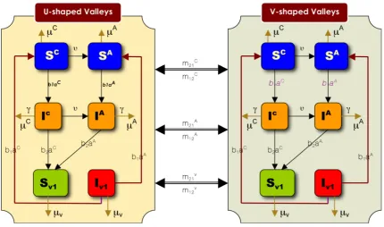
the proportion of individuals travelling from from patch i to patch j. The flow of individuals into the

different compartments is represented in Figure 1. We use i to represent the U-shaped valleys and j the V-shaped valleys. Due to the heterogenous nature of malaria in Western Kenya highlands, there are other patches characterized by other features not necessarily the ecosystem, hence the numbering i=1,,n.

The total host population on patch i is defined as C A

i i i

N =N +N and its dynamics by N_i′ =

( ) ( )

N_iC ′+ N_iA ′, with

( )

1, 1,

n n

C C C C C

i ij j ji i

j j i j j i

n n

A A A A A

i ij j ji i

j j i j j i

N m N m N

= ≠ = ≠

′ = −

∑

(3)

[image:3.595.100.531.83.337.2]

Figure 1. Transfer diagram for the different epidemiological groups in different patches.

where 1,

n j j= j i≠N

∑

is the total number of residents of patch i at time t [14].

We define the vectors NC, NA , and V in n +

 . The matrix MC is

,

1,

if otherwise

C ij C

n i j C C

ii ji j j i

m i j

M

m m

= ≠

 ≠

 = 

= − 



∑

(2)

and the matrix MA analogously. Equation (1) becomes

( )

_NC ′

( )

_t =_MC

( ) ( )

_{t N}C _t

( )

_NA ′

( )

_t =_MA

( )

_{t N}A

( )

_t The total population of mosquitoes V satisfies,

( )

v

( ) ( )

V t′ =M t V t

If all the patches are sufficiently distant from each other, then mosquitoes do not migrate and Mv

( )

t =0

The dynamics of the total host and vector populations on patch i is

( )

Ni

( )

t Ni

( )

t

∆ ′ ₌_ ∆ ₍₃₎

where N∆ is the vector defined by

C A

N

N N

V ∆

    =      

and the matrix  is the diagonal block matrix

0 0

C A

v

M M

M

 

 

=  

 

 

(4)

The migration equation becomes

( )

( ) ( )

.

N t′ = t N t (4)

We denote

• Λ_i

( )

t is the recruitment of new born children in patch i;

• S_{h i}_,

( )

t the susceptible host population and I_{h i}_,

( )

t the infectious host population in patch i; • S_{v i}_,

( )

t the susceptible vector population and I_{v i}_,

( )

t the infectious vector population in patch i; • a_i the man biting rate of vectors in patch i;

• b₁ the proportion of infectious bites on a host producing a patent infection;

• b₂ the proportion of bites by susceptible vectors on an infected host producing a patent infection; •

µ

_{h i}C_, the head rate of children mortality in patch i,

µ

_{h i}A_, the head rate of adult mortality in patch i;

• 1

ν

the mean duration of childhood;

• µ_{v i}_, the head rate of vector mortality; • c

i

γ the head rate of children recovery from infection, A

i

γ the head rate of adult recovery from infection

and 1

i

γ the mean duration of infection in patch i.

The total host and vector populations are constant in all the patches. The parameter a_i depends on the host

age group in each patch. We also assume that the recovery rate γ_i does not depend on age [5] but on how

quickly the host receives treatment and history of their malaria infection. For patches i=1,,n we have the 6n equations

( )

_{( ) ( )}

( )

(

)

( )

_{( )}

( )

.

, 1 , , , , ,

1, 1,

,

, , 1 , , , , ,

1, 1,

, 1

C n n

C C h i c C C C C C C C

h i i i i v i i h i i h i ij h j h i ji

j j i j j i

i

A _n _n

h i

A C A A A A A A A A A

h i h i i i v i i h i i h i ij h j h i ji

j j i j j i

i

C

h i i

S

S t t b a I t I t S t m S t S t m

N t

S t

S t S t b a I I t S t m S t S t m

N t

I t b a

γ µ ν

ν γ µ

= ≠ = ≠

′ _{= Λ} ₋ ₊ ₋ ₊ ₊ ₋

′ ₌ ₋ ₊ ₋ ₊ ₋ ′ ₌

∑

( )

(

)

( )

_{( )}

( )

(

)

( )

_{( )}

( )

, , , , , 1, 1, ,

, 1 , , , , ,

1, 1,

,

, ( ) 2 , 2

C _n _n

h i

C c C C C C C C

i v i i i h i ij h j h i ji

j j i j j i

i

A _n _n

h i

A A C A A A A A A A

h i i i v i h i i i h i ij h j h i ji

j j i j j i

i

h i C C

v i v i i h i i

i

S t

I t I t m I t I t m

N t

S t

I t b a I t I t I t m I t I t m

N t

S t

S t t b a I t b a

N t

γ µ ν

ν γ µ

= ≠ = ≠

− + + + −

′ ₌ ₊ ₋ ₊ ₊ ₋

′ _{= Λ} ₋ ₊

∑

( )

(

)

( )

_{( )}

( )

(

( )

)

( )

, , , , , 1, 1, ,

, 2 , 2 , , , ,

1, 1,

n n

A A v v

i h i v i v i ij v j v i ji

j j i j j i

n n

h i C C A A v v

v i i i h i i i h i v v i ij v j v i ji

j j i j j i

i

I t S t m S t S t m

S t

I t b a I t b a I t I t m I t I t m

N t µ µ = ≠ = ≠ = ≠ = ≠                 − + −   ′  ₌ ₊ ₋ ₊ ₋ 

∑

(5)

The term Λ_i

( )

t represents the recruitment of newborns into the susceptible children’s class, while

( )

, 1 , C h i C i v i

i

S t b a I

N t in the first equation represents the differentiated infection of susceptible children by infec-

tions mosquitoes using frequency dependent transmission and a non constant host population in patch i. The

term −

γ

_icI_{h i}C_,

( )

t defines the recovery of infected children in patch i. The term C i

µ is the per capita death rate of children in patch i, ν is the rate children pass into adulthood, and the last term defines host migration. For the second and third equations the terms are defined similarly for Adults. In the sixth equation, for infectious vectors, the first term corresponds to the infection of susceptible mosquitoes by infected children and infected adults, while the last term −µ_{i v i}I_,

( )

t caters for vector mortality.

We will assume in the sequel that c

i

ν γ< for any index i

(5)

than the mean sojourn time in the compartment of childhood. Actually 1 1

5 365 j

ν

_≈ −

× and

1

1 2 30

i j

γ

_≈ −

×

The complete system is given by Equations (4) and (5).

3. Reduced System

It turns out that system given by Equation (5) can be rewritten in a triangular form so we need the following theorem to reduce such a system and thus study a smaller system.

Theorem 3.1 (Vidyasagar) Consider the following _1_system_:

( )

(

)

( )

(

)

* *

* * *

, ,

with an equilibrium point, , i.e 0 and , 0

n m

x f x x y y g x y

x y

f x g x y  ′ = ∈ ∈  ′ =

  

 ₌ ₌



 

(6)

If x* is globally asymptotically stable (GAS) in n for the system x′ = f x

( )

, and if *

y is GAS in n, for the system y′ =g x y

( )

*, , then

(

x y*, *

)

is (locally) asymptotically stable for (6). Moreover if all the trajectories of (6) are forward bounded, then

(

x y*, *

)

is a GAS for (6).

To apply the above Vidyasagar theorem we would need to prove the stability analysis of first equation, then we would only have to test the stability of the infection equation.

From Equation (5) if we add the first and third equation together we get

( )

,

(

,

)

1, 1,

n n

C C C C C C C

i h i h i i ij j ji i j j i j j i

N µ ν N m N m N

= ≠ = ≠

′ = Λ − + +

∑

−

∑

Which gives

( )

C

(

diag

(

C 1

)

C

)

C.

h h

N ′ = Λ + −

µ

+ ⋅ +

ν

M N

We note that the matrix −diag

(

µhC+ ⋅ +ν 1

)

MC≥0, is a Metzler matrix.

For a matrix M the stability modulus, that we will denote s M

( )

, is the largest real part of the elements of the spectrum Spec

( )

M of M

( )

_{( )}

( )

Spec

max Re .

M

s M

λ∈ λ

=

We have now

(

)

(

)

T

1 _−diag µ_hC+ ⋅ +ν 1 MC_= − µ_hC+ν 0.

This proves that the stability modulus of MC satisfies

(

)

(

diag Ch 1 C

)

0,

s − µ + ⋅ +ν M <

implying that this Metzler matrix is non singular, which in turn implies the opposite, that is, its inverse is nonnegative [15] [16]. Therefore the equilibrium of this linear system is given by

(

)

1

diag 1 0,

C C C

h h

N = − −_ µ + ⋅ +ν M _− Λ >

and is globally asymptotically stable.

A similar result is obtained for the adult population with an equilibrium denoted by NA

( )

(

)

1

diag 0,

A A A C

N = − −ν µ +M − N >

and for the mosquito population with an equilibrium denoted by V.

( )

(

)

1

diag _v v _v.

(6)

Reduction Process

We will now give different expressions for the equation of our system. Depending on the case at hand we will use the most convenient form to give the properties of this system and the corresponding proofs.

Using β =₁_i b a₁ _i, and β =₂_i b a₂ _i, we can rewrite system (5) in 6n +

 , with an immediate variable change

( )

(

)

( )

(

( )

)

( )

(

)

( )

(

( )

_{( )}

( )

)

(

)

( )

(

( )

_{( )}

( )

)

( )

(

)

,

, 1 , , , ,

1, 1,

,

, 1 , , ,

diag 1

diag

1

C C C C

h

A C A A A

h

v

v v

C C

n n

i h i

C C C C C C C C

h i i v i i h h i ij h j h i ji

j j i j j i

i

A A

i h i

A A C A A

h i i v i h i i i h i

i

N M N

N N M N

V M V

N t I t

I t I t I t m I t I t m

N t

N t I t

I t I t I t I

N t µ ν

ν µ

µ

β γ µ ν

β ν γ µ

= ≠ = ≠

′ = Λ + − + ⋅ +

′ = + − +

′ = Λ + − +

− ′ ₌ ₋ ₊ _{+ ⋅} ₊ ₋ − ′ ₌ ₊ ₋ ₊

∑

( )

(

( )

_{( )}

( )

)

(

( )

)

( )

, , 1, 1, ,

, 2 , 2 , , , ,

1, 1,

n n

A A A A

ij h j h i ji

j j i j j i

n n

i v i C C A A v v

v i i h i i h i v v i ij v j v i ji

j j i j j i

i

t m I t I t m

V t I t

I t I t I t I t m I t I t m

N t β β µ

= ≠ = ≠ = ≠ = ≠              + −    ₋ ′  ₌ ₊ ₋ ₊ ₋ 

∑

(7)

This system is clearly triangular if we consider the first variables

(

NC

( )

t ,NA

( ) ( )

t V t,

)

. By application of Theorem (3.1), the stability analysis of (7) is now reduced to the stability analysis of the system

( )

(

( )

_{( )}

( )

)

(

)

( )

(

( )

)

( )

(

)

( )

(

( )

)

,

, 1 , , , ,

1, 1,

,

, 1 , , , , ,

1, 1, , , 1 ( ) C C n n

i h i

C C C C C C C C

h i i v i i h h i ij h j h i ji

j j i j j i

i

A A

n n

i h i

A A C A A A A A A

h i i v i h i i i h i ij h j h i ji

j j i j j i

i

i v i

v i

i

N t I t

N t

N t I t

I t I t I t I t m I t I t m

N

V t I t I t

N t

β γ µ ν

β ν γ µ

= ≠ = ≠ = ≠ = ≠ − ′ ₌ ₋ ₊ _{+ ⋅} ₊ ₋ − ′ ₌ ₊ ₋ ₊ ₊ ₋ − ′ ₌

∑

( )

(

2 , 2 ,

)

,

( )

,

( )

,

( )

1, 1,

n n

C C A A v v

i h i i h i v v i ij v j v i ji

j j i j j i

β β µ

= ≠ = ≠          ₊ ₋ ₊ ₋  

∑

(8) We set C A

N=N +N

(

)

T

,1, ,2, , ,

C C C C

h h h h n

I = I I  I

(

)

T

,1, ,2, , ,

A A A A

h h h h n

I = I I  I

(

)

T

,1, ,2, , ,

v v v v n

I = I I  I

(

)

T

(

)

T

1 11, 12, , 1 , 1 11, 12, , 1

c c c c A A A A

n n

β = β β  β β = β β  β

(

)

T

(

)

T

2 21, 22, , 2 , 2 21, 22, , 2

c c c c A A A A

n n

β = β β  β β = β β  β

(

)

T

(

)

T

1 , 2 , , , 1 , 2, ,

C C C C A A A A

n n

γ = γ γ γ γ = γ γ γ

Then Equation (8) can be written, in a vectorialized way, as

( )

(

)

(

)

( )

(

)

(

)

( )

(

)

(

)

( ) (

)

( )

1 1 1 1 1

2 2 ,

diag diag diag diag 1

diag diag diag diag

C C C C C C C C C

h h v h h h

A A A A C A A A A A

h h v h h h h

C C A A v

v h h i v i v v v

I N N I I I M I

I N N I I I I M I

I I I N V I I M I

β γ µ ν

β ν γ µ

β β µ

(7)

For another variable change, we set

( )

1

diag C C

h

x= N − I

( )

1

diag A _hA

y= N − I

( )

1

diag v.

z= V − I

Rewriting system (9) in terms of x, y and z, we have

( )

(

)

(

)

( )

(

)

(

)

( )

( ) ( )

( )

( ) ( )

( ) (

)

( )

1 1 1 1 1 2 2

diag diag diag diag 1 diag 1

diag diag diag diag 1 diag

diag diag diag diag diag diag diag 1 diag ,

C C C C

h

A A A A

h

C C A A v

v

x N V x z x M x

y N V y z y x M y

z N N x N y z z M z

β γ µ ν

β β µ

− − −  ′ = − − + + ⋅ +   ′ = − − + + +      ′ = _ + _ − − +     (10)

where we define the matrices

( )

1

( )

diag diag ,

C C C C

M = N − M N

( )

1

( )

diag diag ,

A A A A

M = N − M N

( )

1

( )

diag diag .

v v

M = V − M V

Finally, we will make a final “vectorization” of the system

( )

1 1 1 1 1

diag diag diag 0 0

0 diag diag diag 0

0 0 diag

C A N V N V N β β − − −       =         

( ) ( )

2

( ) ( )

2

0 0

diag diag diag diag 0

n n

C C A A

I I N N β β       =       

(

)

(

)

( )

diag 1 0 0

diag 0

0 0 diag

C C h A A n h v I γ ν µ

ν γ µ

µ  + ⋅ +      = − +        0 0 0 0 0 0 C A v M M M     =           

We observe that  = ∆−1∆ where ∆ is the diagonal matrix

( )

diag 0 0

0 diag 0

0 0 diag

C A N N V       ∆ =      

(8)

( )

min

(

1 _hC, _hA, _v

)

0

s − = −

γ ν

+ ⋅ +

µ γ µ µ

+ <

where the minimum is taken over the components of the 3 positive vectors. We have

( )

3n

s I

− +  ≤ −  +

Since the matrices involved are Metzler matrices, this implies the following inequality for the corresponding stability modulus

(

)

( )

3n

( )

0

s − +  ≤ −s  I +s  = −s  <

The relation s

( )

 follows from s

( )

 =s

( )

 and from T

1 =0 which implies by Perron-Frobenius

that s

( )

 =0.

Using the preceding matrices and the vector X =

(

x y z, ,

)

we rewrite Equation (10) in a compact form as

(

)

(

)

diag 1

X′ = −X X + − +  X (11)

This system evolves on the unit cube of 3n.

4. Basic Properties of the Model

For any index i we shall use the classical notations: x< y if x≤ y and x_i≤y_i for some i and we write

i i

x  y if x_i<y_i for all i.

Proposition 4.1 (Positively Invariant Set)

The unit cube

(

)

{

3

}

, , n 0 1; 0 1, 0 1 .

x y z x y z

= ∈ ≤ ≤ ≤ ≤ ≤ ≤ K

is positively invariant for system (10).

Proof

To show the invariance of the unit cube K, under the flow of the system (10), it suffices to show that each of the faces of the cube cannot be crossed.

On the patch i we have

(

)

(

)

1 ,

1, 1,

1

C

n n

j

C i C C C C

i i i i i h i i ij C j i ji j j i j j i

i i

N V

x z x x m x x m

N N

β

γ

µ

ν

= ≠ = ≠

′ = − − + + +

∑

−

∑

If xi =0

1

1,

0.

C n

j C i C i i i ij C j

j j i

i i

N V

x z m x

N N

β

= ≠

′ = +

∑

≥

implying that x=0 cannot be crossed from positive to negative. If xi =1 we have

(

,

)

1, 1,

C

n n

j

C C C C

i i h i ij C j ji j j i i j j i

N

x m x m

N

γ

µ

ν

= ≠ = ≠

′ = − + + +

∑

−

∑

The relation xi =1 is equivalent to ,

C C h i i

I =N . But C

N is a demographic equilibrium satisfying

(

)

(

−diag µhC+ ⋅ +ν 1 MC

)

NC = −Λ

Taking this fact into account gives

(

,

)

1, 1,

,

n n

C C C C C C i h i i ij j i ji

j j i j j i

N m N N m

µ ν

= ≠ = ≠

−Λ = − + +

∑

−

∑

(9)

( )

1

(

)

,

1, 1,

,

C

n n

j

C C C C

i i h i ij C ji j j i i j j i

N

N m m

N

µ

ν

−

= ≠ = ≠

− Λ = − + +

∑

−

∑

which gives in turn, since xj ≤1

( )

1

0.

C C

i i i i

x′ ≤ −γ − N − Λ <

The equation for y_i in patch i is

(

)

(

)

1 ,

=1, =1,

1

A

n n

j

A i A A A A

i i i i i h i i ij A j i ji j j i j j i

i i

N V

y z y y m y y m

N N

β

γ

µ

≠ ≠

′ = − − + +

∑

−

∑

If yi =0 then

1

1,

0.

A n

j A i A i i i ij A j

j j i

i i

N V

y z m y

N N

β

= ≠

′ = +

∑

≥

if yi=1 a similar argument, as for the case xi=1 gives

( )

1

0.

A C

i i i i

y′ ≤ − −γ ν N − N <

Finally the equation for z_i in patch i is given by

(

)

(

)

2 2 ,

1, 1,

1 1

C A n n

j

C i A i v v

i i i i i v i i ij j i ji j j i j j i

i i i

V

N N

z x z y z z m z z m

N N V

β

µ

= ≠ = ≠

′ = − + − − +

∑

−

∑

If zi=0, then for any i,

2 2

1,

0,

C A n

j C i A i v i i i i i ij j

j j i

i i i

V

N N

z x y m z

N N V

β

= ≠

′ = + +

∑

≥

and if zi=1 a similar argument, as for the cases x1=1 and yi=1 gives

( )

1

, 0.

i i v i

z′ ≤ − V − Λ ≤

The proposition is proved.

Proposition 4.2

If the matrix C A v

M +M +M is irreducible, then the system (11) is strongly monotone in the interior of the

positively invariant set

[ ]

0,13n

Proof

We utilise the theory of monotone dynamical systems introduced by [17] [18], developed further in [19] and applied in [10].

System (11) is monotone if its Jacobian is a Metzler matrix on the unit cube. The Jacobian of system (11) is given by

( )

diag 1

(

)

(

)

diag

( )

J X = −X + − +   − X

The Jacobian J X

( )

is clearly a Metzler matrix since 0≤X ≤1, which implies that the system is

cooperative in the unit cube.

Next, we show that the Jacobian J X

( )

is an irreducible matrix in the set

[ ]

0,13n. This will imply strong monotonicity of the system in the interior of the unit cube. In this set the diagonal terms of diag 1

(

−X

)

are positive, the same property is satisfied for , then the connectivity of the associated graph of diag 1

(

−X

)



is reduced to the connectivity of .

It is well known that a matrix is irreducible if its associated graph is strongly connected. Then only the off diagonal terms are concerned. Then it is sufficient to prove that the matrix

(

)

(

)

diag 1−X + − + 

   

(10)

the x_i (children vertices), y_i (adults vertices), z_i (mosquitoes vertices). Considering the matrix  it is clear that a vertex x_i is connected to the vertices of the same patch i, i.e., y_i and z_i. In other words on the

three vertices of patch i are contained in a strongly connected component. The vertices from a patch is a

subgraph and we can use the contraction of each

(

x y zi, i, i

)

in the general digraph to obtain a new digraph

which represents movements between the patches. To prove the strong connectedness, it is sufficient to prove that this contracted digraph is strongly connected.

To the matrix , there is a corresponding digraph between the patches. This graph is equivalent to the

associated digraph of C. Since MC, MA and Mv are Metzler matrices, we can consider the matrix

C A v

M +M +M and its corresponding multigraph on the graph of patches. This oriented multigraph represents

actually the circulation of malaria parasites between the patches. Malaria parasites can be transported either by child, adults or mosquitoes.

Since we have assumed that the matrix is irreducible, our graph is strongly connected, consequently the Jacobian is irreducible. We note that we are in a context of multiple species (i.e., childs, adults and mosquitoes) in a metapopulation model as conceptualized in [20].

Our assumption simply means that the circulation of parasites is strongly connected.

:

NB The establishment of the equilibrium solution and study of stability for the disease free and the

endemic equilibrium will be tackled in a forth coming article.

5. Conclusions

In this study, we formulated an infinite model representing the spread of malaria in a heterogenous population classified. This population is classified as children (0 - 5 years) and adults (above 5 years). The infectivity and susceptibility of the population to highland malaria depend on: 1) the age class and; 2) the type of ecosystem the individual inhabits. The study captures the role played by the age of the individual and the ecosystem heterogeneity in malaria epidemically spreading in the regions called patches. Hats are defined depending on their topography. Model properties are described to show that the solution set exists in the positive orthant which is

positively invariant. The system is reduced to a single equation in 3n, which is strongly connected and

strongly monotone. The large scale system has been reduced using vectorialization into a compact form which is easier to study. The establishment of equilibrium solution and stability study will be done in a forthcoming article.

Acknowledgements

We wish to acknowledge of the Inria Metz, UMMISCO(IRD), the French Embassy in Nairobi and the Uni- versity of Nairobi, Kenya, for their financial, logistic and moral support during the writing of this article. We are very grateful to Dr. Githeko, KEMRI Kisumu for the great insight and literature he gave us during this study.

References

[1] Vidyasagar, M. (1980) Decomposition Techniques for Large Scale Sytems with Nonadditive Interactions: Stability and Stabilization. IEEE Transactions on Automatic Control, 25, 773-779. http://dx.doi.org/10.1109/TAC.1980.1102422

[2] Githeko, A.K., Ayisi, J.M., Odada, P.K., Atieli, F.K., Ndenga, B.A., Githure, J.I. and Yan, G. (2006) Topography and Malaria Transmission Heterogeneity in Western Kenya Highlands: Prospects for Focal Vector Control.Malaria Jour- nal, 5, 107. http://dx.doi.org/10.1186/1475-2875-5-107

[3] Wolfgang, M.R., Willem, T., Richard, C. and Bart, K. (2002) Host-Specific Cues Cause Differential Attractiveness of Kenyan Men to the African Malaria Vector Anopheles Gambiae. Malaria Journal, 1, 17.

http://dx.doi.org/10.1186/1475-2875-1-17

[4] Smith, D.L., Guerra, C.A., Snow, R.W. and Simon, H.I. (2007) Standardizing Estimates of the Plasmodium Falciparum Parasite Rate. Malaria Journal, 6, 131. http://dx.doi.org/10.1186/1475-2875-6-131

[5] Tumwiine, J., Mugisha, J.Y.T. and Luboobi, L.S. (2007) On Oscillatory Pattern of Malaria Dynamics in a Population with Temporary Immunity. Computational and Mathematical Methods in Medicine, 8, 191-203.

[6] Wanjala, C.L., Waitumbi, J., Zhou, G. and Githeko, A.K. (2011) Identification of Malaria Transmission and Epidemic Hotspots in the Western Kenya Highlands: Its Application to Malaria Epidemic Prediction. Parasites and Vectors, 4, 81. http://dx.doi.org/10.1186/1756-3305-4-81

(11)

and Engineering, 3, 89-100. http://dx.doi.org/10.3934/mbe.2006.3.89

[8] Pongsumpun, P. and Tang, I.M. (2003) Transmission of Dengue Haemorrhagic Fever in an Age Structured Population. Mathematical and Computer Modeling, 37, 949-961. http://dx.doi.org/10.1016/S0895-7177(03)00111-0

[9] Gao, D. and Ruan, S. (2012) A Multipatch Malaria Model with Logistic Growth Populations. SIAM: SIAM Journal on Applied Mathematics, 72, 819-841. http://dx.doi.org/10.1137/110850761

[10] Auger, P., Kouokam, E., Sallet, G., Tchuente, M. and Tsanou, B. (2008) The Ross-Macdonald Mode in a Patchy Envi- ronment. Mathematical Biosciences, 216, 123-131. http://dx.doi.org/10.1016/j.mbs.2008.08.010

[11] Ross, R. (1911) The Prevention of Malaria. Springer-Verlag, Berlin.

[12] Lutambi, A.M., Penny, M.A., Smith, N. and Chitnis N. (2013) Mathematical Modeling of Mosquito Dispersal in a He- terogenous Environment. Mathematical Biosciences, 241, 198-216.

[13] Kelly, D.W. and Thompson, C.E. (2000) Epidemiology and Optimal Foraging: Modelling the Ideal Free Distribution of Insect Vectors. Parasitology, 120, 319-327.

[14] Arino, J, Davis, J.R., Hartley, D., Jordan R., Miller, J. and van den Driessche, P. (2005) A Multispecies Epidemic Model with Spatial Dynamics. Mathematical Medical Biology, 22, 129-142.

[15] Berman, A.P. and Robert, J. (1979) Nonnegative Matrices in the Mathematical Sciences, Volume 9 of Classics in Ap- plied Mathematics. Society for Industrial and Applied Mathematics (SIAM), Philadelphia. Revised Reprint of the 1979 Original.

[16] Smith, H.L. (1995) Monotone Dynamical Systems: An Introduction to the Theory of Competitive and Cooperative Systems, Volume 41. Mathematical Surveys and Monographs.

[17] Hirsch, M.W. (1982) Systems of Differential Equations That Are Competitive or Cooperative I: Limit Sets. SIAM: SIAM Journal on Applied Mathematics, 13, 167-179. http://dx.doi.org/10.1137/0513013

[18] Hirsch, M.W. (1988) Systems of Differential Equations That Are Competitive or Cooperative III: Competing Species. SIAM: SIAM Journal on Applied Mathematics, 1, 51-71.

[19] Hirsch, M.W. and Smith, H.L. (2005) Monotone Dynamical Systems. Handbook of Differential Equations: Ordinary Differential Equations. Vol. II, Elsevier B. V., Amsterdam, 239-357.