A Semi Supervised Technique for Weather Condition Prediction using DBSCAN and KNN

(1)

A Semi- Supervised Technique for Weather Condition

Prediction using DBSCAN and KNN

Aastha Sharma

M-tech Research Scholar

CSE Department TIT, Bhopal

Setu Chaturvedi

, Ph.D Assist. Professor & Head

CSE Department TIT, Bhopal

Bhupesh Gour

, Ph.D Professor CSE Department

TIT, Bhopal

ABSTRACT

Weather condition prediction has always been a keen area of interest among researchers and climate change prediction experts. Due to gradual changes in the atmospheric and climatic conditions the appropriate prediction task has become a formidable challenge. In this paper we propose a semi- supervised weather prediction technique to validate the predictions done for certain atmospheric parameters taken for four years on a day wise basis in a certain city. The experimental outcomes of this work show that this semi supervised technique provides appropriate results and can be used for weather condition prediction & analysis.

Keywords

Clustering, DBSCAN, Data mining, KNN, Semi-Supervised.

1. INTRODUCTION

Weather condition can be described as the state of the atmosphere at a given time and place. Troposphere is the lowest layer of the atmosphere, which is responsible for changes in the weather conditions. Meteorologists [1] and scientists are constantly studying and describing weather in a series of ways. Weather forecasting [2] entails predicting how the present state of the atmosphere will change. It has been one of the most scientifically and technologically challenging problems around the world in the last century. This is due to mainly two factors: first, it is used for many human activities and secondly, due to the opportunism created by the various technological advances that are directly related to this concrete research field, like the evolution of computation and the improvement in measurement systems. To make an accurate prediction [3] is one of the major challenges facing meteorologist all over the world. Since ancient times, weather prediction has been one of the most interesting and fascinating domain. Scientists have tried to forecast meteorological characteristics [4] using a number of methods, some of these methods being more accurate than others.

Artificial intelligence has a type of subfield commonly known as machine learning [5]. In this technique, algorithms and methods are created that allow computers to learn from them. This provides ability to computers so that they can learn from analytical observations, pre-experiences and other means, resulting in a system that can has ability to endlessly improve itself so that the overall efficiency of the system can be improved. Learning is about generality.

There are two types of learning: 1 .Inductive learning 2. Transductive learning.

The objective of inductive learning is to develop a classifier that is good enough with the capacity to simplify any unseen data and train the given dataset efficiently. During the time of training the learner has no knowledge about the test dataset.

However, in Transductive learning the test dataset is very well known to the learner during the time of training and therefore it only requires to make a good classifier that generalizes to this known test dataset.

One common learning approach is supervised learning [6]. In supervised learning provides mechanisms for training dataset comprising of only labeled data. The name ‘supervised’ specifies the fact that the learner is provided with the necessary labeled data. However, the motive is to learn a function which is capable to generalize well on unseen and unlabeled data so, another method is unsupervised learning. In this method only a part of sample data is offered or provided to the system as observations without any label. Unsupervised learning [6] uses processes that try to find the regular patterns of the data. In unsupervised methodology there is no external guidance given to the system to locate the pattern of the model and it is the responsibility of the learner itself to find out the required actions. In supervised learning the training dataset given is entirely labeled, however in unsupervised learning, none of the training dataset is labeled. Semi-supervised learning [7] is the technique of finding a better classifier, when it is provided with both labeled and unlabeled data. Semi-supervised learning methodology can deliver high performance of classiﬁcation by utilizing unlabeled data. The methodology can be used to adapt to a variety of situations by identifying as opposed to specifying a relationship between labeled and unlabeled data from data. It can achieve improvement when unlabeled data can reconstruct the optimal classiﬁcation boundary. Some popular semi- supervised learning models include self-training, mixture models, graph-based methods, co-training and multi-view learning. The success of semi- supervised learning depends completely on some underlying assumptions. So the emphasis is on the assumptions made by each model.

(2)

2. DATA DESCRIPTION

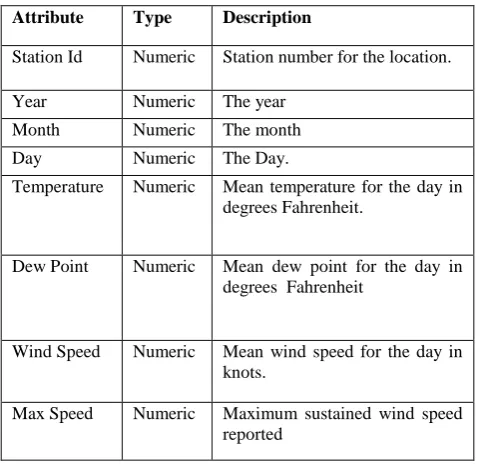
[image:2.595.48.289.217.449.2]

The data summaries provided here are based on data exchanged under the World Meteorological Organization (WMO) World Weather Watch Program according to WMO Resolution 40.The collected data has been pre- processed and has been normalized to 10%. Out of this 10% of processed data 70 % of it has been given as the training data to the algorithm. Rest 30% has been used to be classified using the semi-supervised technique to the classes made using the DBSCAN algorithm [8]. Table 1.Gives the description of the attributes used in the learning process.

Table 1. Data description

Attribute Type Description

Station Id Numeric Station number for the location.

Year Numeric The year Month Numeric The month Day Numeric The Day.

Temperature Numeric Mean temperature for the day in degrees Fahrenheit.

Dew Point Numeric Mean dew point for the day in degrees Fahrenheit

Wind Speed Numeric Mean wind speed for the day in knots.

Max Speed Numeric Maximum sustained wind speed reported

for the day in knots

3. PROPOSED WORK

In this paper we propose a new approach that combines data-mining technologies like classification [11] and clustering [12]. Figure 1 Shows that the sample dataset that has to be trained is given as input to Semi- supervised clustering algorithm. The Semi-supervised algorithm can identify clusters in large spatial data sets by looking at the local density of database elements using only input parameter. After clusters are formed, they are given for training to KNN. K-nearest Neighbour rule (KNN) [9] has been one of the most well-known supervised learning algorithms in pattern classification Thus the whole approach is termed as semi-supervised clustering [10] methodology that is used for prediction of weather attributes like snow, Rain and Fog.

Fig 1: Proposed Architecture of Semi Supervised Technique

1. The proposed semi-supervised technique is categorized into two parts:

i. Clustering: A clustering algorithm has been employed to partition a training data set. Clustering is a data mining technique which is used to group large sets of data into clusters of small sets of similar data. DBSCAN algorithm has been used for clustering the training dataset.

ii. Classification: After the data has been clustered, we applied a classification technique to obtain a mapping from the clusters to the different known classes the result of the learning is a set of cluster.

3.1 Proposed Algorithm

1. Load training Data set d={stdid, year, day, month, temp, dewp , wdsp, mxspd, FRHSTT;}.

2. Calculate the D(Eps,MinPts) Respectively.

NEps(p) = {q ϵ D|dist(p,q)<Eps} where p: border point q: core point.

3. Clusters will generate on the basis of above Step 2 i.e C1, C2, C3………,Cn.

And assign Id to each clusters custid=1 to custid=n. 4. For Each clusters Ci apply the k=i1, i2, i3………in and

calculate the Euclidean distance is the straight-line distance between two points , where (x1,y1) & (x2,y2) are

√((x1 - x2)² + (y1 - y2)²)

5. On the basis of Test Data Set rearrange the clusters into Rain, Snow and Fog class.

6. Finalize the output.

4. EXPERIMENTAL RESULTS

Density-Based Spatial Clustering and Application algorithm has been used to cluster data. It did clustering through growing high density area. Evaluation of the performance of the proposed system is an important and mandatory issue, so the overall accuracy of the system has been evaluated.

Following are the evaluation parameters that has been considered in performance evaluation:

1. Overall Accuracy. 2. Class wise Accuracy. 3. Class wise Precision. 4. Class wise Recall. 5. Class wise F-measure.

Metrics Applied:Following metrics have been applied to the semi-supervised classifiers:

TP (True Positive):-For a given class, the number of correctly classified objects is referred to as a True Positive (TP).

FP (False Positive):- The number of objects falsely identified as a class is referred as a False Positive (FP).

FN (False Negative):-The number of objects from a class that are falsely labelled as another class is referred as False Negative (FN).

TN (True Negative):- For a given class, the number of incorrectly classified objects.

Input Training Sample Data Test Data

Set

Finalized Output

DBSCAN Clustering

Algorithm KNN→C

[image:2.595.65.271.628.727.2]

(3)

Table 2. Confusion Matrix

Accuracy: - Accuracy may be defined as ratio of Sum of True Positive and True Negative to the sum of all True and False Positive, True and False Negative for all classes

Precision: - Precision is the ratio of True positives to True and False Positives. This determines how many identified objects were correct.

Recall: - Recall is the ratio of True Positives to the number of True Positives and False Negatives. This determines how many objects in a class are misclassified as something else.

F-measure: - F measures the balance between precision and recall; it is harmonic mean between them.

4.1 Experimental outcomes

The validity of the experimental results can be described with the help of confusion matrices. Following are the confusion matrices based on the actual values and the predicted values for the various classes considered in this paper. The results are based on different values of k.In this paper basically consider three classes FOG, RAIN and SNOW on the basis of Following parameters we predicate the weather conditions:

Accuracy= ...Eq. (1)

Precision= ...Eq. (2)

Recall= ...Eq. (3)

FOG

[image:3.595.319.538.71.158.2]

Table 3 Show the confusion Matrix of our test class FOG. This table contains the comparison between predicated and actual values of TN, FN, TP, FP for different values of K=25, 30,35,40,45 and 50.

Table 3. Confusion matrix of FOG

K=25 Predicted Values

Actual Values 416 0

32 0

64 0

96 0

128 0

160 0

192 0

4.1.1 Accuracy of FOG

Figure 2. Shows the Accuracy of FOG. Graph is plotted between different values of K and the percentage of accuracy achieved for values of K=25, 30,35,40,45 and 50.We observe that the achieved accuracy remains above 90 % for different values of K.

Figure 2: Accuracy of Class FOG

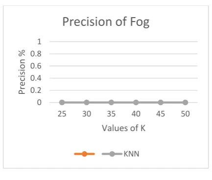
4.1.2 Precision of FOG

:

Figure 3. Show the Precision of FOG. Graph is plotted between different values of K and the percentage of Precision achieved for values of K=25, 30,35,40,45 and 50.We observe that the achieved Precision remains 0 % for different values of K.

Figure 3. Precision of Class FOG

4.1.3 Recall of FOG:

Figure 4. Shows the Recall of FOG. Graph is plotted between different values of K and the percentage of Recall achieved

0 20 40 60 80 100

25 30 35 40 45 50

Acc

u

ra

cy

%

Values of K

Accuracy of Fog

KNN

0 0.2 0.4 0.6 0.8 1

25 30 35 40 45 50

Prec

is

ion

%

Values of K

Precision of Fog

KNN Class P’ (Predicted) N’ (Predicted)

P (Actual) True Negative(TN) False Positive (FP) N

(Actual)

[image:3.595.52.255.95.155.2] [image:3.595.320.537.254.428.2] [image:3.595.320.537.519.703.2] [image:3.595.61.276.590.767.2]

(4)

for values of K=25, 30,35,40,45 and 50.We observe that the achieved Recall remains 0 % for different values of K.

Figure 4. Recall of Class FOG

RAIN

[image:4.595.329.527.70.265.2]

Table 4. Shows the confusion Matrix of our test class Rain. This table contains the comparison between the predicated and actual values of TN, FN, TP, FP for different values of K=25, 30,35,40,45 and 50.

Table 4. Confusion matrix of RAIN

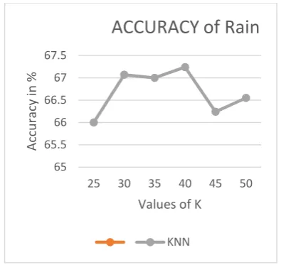
4.2.1 Accuracy of RAIN

Figure 5.Show the Accuracy of Rain. Graph is plotted between different values of K and the percentage of accuracy achieved for values of K=25, 30,35,40,45 and 50.We observe that the achieved accuracy remains above 67 % for different values of K.

Figure 5. Accuracy of Class RAIN

4.2.2 Precision of RAIN:

Figure 6. Show the Accuracy of RAIN. Graph is plotted between different values of K and the percentage of Precision achieved for values of K=25, 30,35,40,45 and 50.We observe that the achieved precision remains above 67 % for different values of K.

Figure 6. Precision of Class RAIN

4.2.3 Recall of RAIN

Figure 7. Show the Recall of RAIN. Graph is plotted between different values of K and the percentage of Recall achieved for values of K=25, 30,35,40,45 and 50.We observe that the achieved recall remains above 80 % for different values of K. 0

0.2 0.4 0.6 0.8 1

25 30 35 40 45 50

Re

call %

Vaues of K

Recall of Fog

KNN

65 65.5 66 66.5 67 67.5

25 30 35 40 45 50

Ac

curacy

in

%

Values of K

ACCURACY of Rain

KNN

65.5 66 66.5 67 67.5 68 68.5

25 30 35 40 45 50

Prec

is

ion

in

%

Values of K

Precison of Rain

KNN

Actual Values

102 94

58 194

196 196

99 405

310 278

165 591

404 380

207 801

516 464

293 967

606 570

[image:4.595.58.276.101.285.2] [image:4.595.327.528.362.536.2] [image:4.595.60.275.390.654.2]

(5)

Figure 7. Recall of Class RAIN

[image:5.595.64.269.67.239.2] [image:5.595.313.526.69.238.2]

SNOW

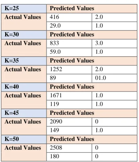
[image:5.595.328.543.327.493.2]

Table 5. Show the confusion Matrix of our test class SNOW. This table contains the comparison between predicated and actual values of TN, FN, TP, FP for different values of K=25, 30,35,40,45 and 50

Table 5. Confusion matrix of SNOW

Actual Values 416 2.0

29.0 1.0

59.0 1.0

89 01.0

119 1.0

149 1.0

180 0

4.3.1 Accuracy of SNOW

Figure 8. Show the Accuracy of SNOW. Graph is plotted between different values of K and the percentage of accuracy achieved for values of K=25, 30,35,40,45 and 50.We observe that the achieved accuracy remains above 93% for different values of K.

Figure 8. Accuracy of Class SNOW

4.3.2 Precision of SNOW

Figure 9. Shows the Precision of SNOW. Graph is plotted between different values of K and the percentage of precision achieved for values of K=25, 30,35,40,45 and 50.

Figure 9. Precision of Class SNOW

4.3.3 Recall of SNOW:

Figure 10. Show the Recall of SNOW. Graph is plotted between different values of K and the percentage of recall achieved for values of K=25, 30,35,40,45 and 50.

Figure 10. Recall of Class SNOW

74 76 78 80 82

25 30 35 40 45 50

Re

call in

%

Values of K

Recall of Rain

KNN

92.8 93 93.2 93.4 93.6

25 30 35 40 45 50

Acc

u

ra

cy

%

Values of K

Accuracy of Snow

KNN

0 1 2 3

25 30 35 40 45 50

Re

call %

Values of K

Recall of Snow

KNN 0

10 20 30 40

25 30 35 40 45 50

Prec

is

ion

%

Values of K

Precision of Snow

[image:5.595.54.281.342.606.2] [image:5.595.315.528.570.733.2]

(6)

5. CONCLUSION

In this paper we applied a Semi-supervised technique comprising DBSCANS and KNN for clustering and classification respectively. This technique derived three classes FOG, RAIN and SNOW. We calculated different metrics for these classes and came to the conclusion that algorithm gives maximum percentage of accuracy at K=40. The dataset has been taken form World Meteorological

Organization (WMO

) and attributes of a single station have been considered. The dataset in this research has approximately 1200 records. After all the experimental analysis we came to a conclusion that Semi- supervised technique can be used for the prediction of meteorological data.

6. REFERENCES

[1] A.B Adeymo, “Soft Computing techniques for weather and Climate change studies ”,African journal Of Computing , Vol 6, No.2, June 2013.

[2] Folorunsho Olaiya, Adesesan Barnabas Adeyemo “Application of Data Mining Techniques in Weather Prediction and Climate Change Studies” I.J. Information Engineering and Electronic Business, 2012, 1, 51-59 [3] Folorunsho Olaiya , Adesesan Barnabas Adeyemo ,

“Application of Data Mining Techniques in Weather Prediction and Climate Change Studies”, I.J. Information Engineering and Electronic Business,February 2012. [4]Casas D. M, Gonzalez A.T, Rodrgíue J. E. A., Pet J. V.,

2009, “Using Data-Mining for Short-Term Rainfall Forecasting”, Notes in Computer Science, Vol. 5518, 487-490

[5] X. Zhu and A. B. Goldberg” Introduction to Semi-Supervised Learn- ing. Synthesis Lectures on Artiﬁcial

Intelligence and Machine Learning’Morgan & Claypool Publishers, 2009.

[6]R. Sathya, Annamma Abraham “Comparison of Supervised and Unsupervised Learning Algorithms for Pattern Classification”(IJARAI) International Journal of Advanced Research in Artificial Intelligence, Vol. 2, No. 2, 2013

[7]V. Jothi Prakash1, Dr. L.M. Nithya2,” A Survey On Semi-Supervised Learning Techniques ”, IJCTT ,Vol 8 No. 1, Feb 2014.

[8] M. Ester, H. P. Kriegel, J. Sander, and X. Xu, "A Density Based Algorithm for Discovering Clusters in Large Spatial Databases with Noise," Proc. Sencond Int'l Conf . Knowledge Discovery and Data Mining(KDD), 1996, pp. 226-231.

[9] Zahoor Jan, M. Abrar, Shariq Bashir, and Anwar M. Mirza” Seasonal to Inter-annual Climate Prediction Using Data Mining KNN Technique” © Springer-Verlag Berlin Heidelberg 2008.

[10]V. Jothi Prakash, Dr. L.M. Nithya”A Survey On Semi-Supervised Learning Techniques” International Journal of Computer Trends and Technology (IJCTT) – Vol. 8 number 1– Feb 2014.

[11]Yujie Zheng, “Clustering Methods in Data Mining with its Applications in High Education “, (ICETC2012)IPCSIT vol.43 (2012) © (2012) IACSIT Press, Singapore