Performance comparison of Different Pilot Aided Channel Estimation Techniques for OFDM IEEE 802 11e (Mobile Wimax) Systems

Performance Comparison of Different Pilot Aided

Channel Estimation Techniques for OFDM IEEE

802.11e (Mobile Wimax) Systems

Rajeshwar Singh

Lovely Professional University Punjab,INDIA

Gurpreet Singh Saini

Lovely Professional University Asst.Professor

ABSTRACT

Orthogonal frequency-division multiplexing (OFDM) modulation is a promising technique for achieving the high bit rates required for a wireless multimedia service. In this paper we present different channel estimation algorithms for OFDM mobile communication systems based on the use of pilot subcarriers. Specifically we present LS (Least Square), MMSE (Minimum Mean Square Error) and LMS iterative channel estimation techniques to show the performance comparison of channel estimation techniques supported by n IFFT-based time channel estimation. The channel estimation is based on the principle of pilot-symbol aided channel estimation (PACE), and it has been implemented using block-type pilot subcarrier arrangements. The low complexity of LMS algorithm, has a higher efficiency than conventional methods (without channel estimation, LS& LMMSE) and it can work in lower amount of SNRs. We have compared the performances of all schemes by measuring bit error rate with 16QAM as modulation scheme, and multi-path Rayleigh fading channel as channel model. Simulation results validate that the LMS Iterative channel estimation scheme can achieve tremendous performance as the existing channel estimation methods.

Keyword:

1. INTRODUCTION

Future generation wireless communication systems demand multiple access schemes with high data transmission capabilities. One such potential multiple access scheme is the Orthogonal Frequency Division Multiple Access. OFDM has received growing interest recently for its use in wireless and wireline communication systems[1] [2]because of its high rate transmission capability with high bandwidth efficiency and robustness to multipath fading and delay. Since OFDM employs overlapped carriers, its spectrum efficiency is also very good. In most of applications, for retaining the orthogonality of subcarriers and overcome intersymbol interference (ISI), a cyclic prefix (CP) is inserted instead of simply inserting guard interval. If the maximum delay of the Multipath channel does not exceed the CP length, the OFDM system would be ISI free by removing the guarding interval. OFDM based systems are strong candidates for air interface of future fourth generation mobile wireless systems which provides high data rate and mobility.

In order to reveal the coherent of received signals, channel coefficients must be estimated by a process so called Channel Estimation. The channel estimation can be performed by inserting pilot sub carriers at the transmitter side and channel coefficients that belong to the pilot subcarriers are estimated using the LS (Least Square) method. Channel estimates are derived [4] from scattered pilots. The pilot carriers in each OFDM symbol contain data known a priori to the receiver. Samples of the channel transfer function can be generated by removing the pilot carrier modulation. Interpolation of these samples can generate the channel estimates for the remaining carriers in the symbol.

Modulation).We evaluate the estimation accuracy of the estimation methods and bit error rate performance. The system with LMS technique provide better results for bit error rate as compared to the LMMSE and LS channel estimators. The LMMSE estimator has good performance but high complexity. The LS estimator has low complexity but its performance is not as good as that of MMSE estimator.LMS technique has less complexity and provide aceeptable BER performance as compared to the other techniques.

2. SYSTEM DESCRIPTION

2.1SYSTEM MODEL

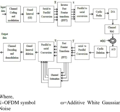
In this section we will examine the transmitter and receiver structure of OFDM systems including the pilot distribution. Consider an OFDM system with N subcarriers which employs the quadrature Amplitude Modulation (QAM) modulation. as illustrated in Figure 1.The vector of data bits is first encoded with an error correcting code such as convolutional code to obtain the vector of coded data bits. This vector is mapped accordingly to the constellations and vector of data symbols is obtained. After the guard band is inserted, an N-point Inverse discrete fourier transform (IDFTn) block transforms the data sequence into time domain. Following the IDFT block, a cyclic extension of time length Tg choosen to be larger than the expected delay spread is inserted to avoid Inter Symbol Interference(ISI) [7-10].The Digital to Analog Converter (D/A) contains low pass filters..The channel is modeled as an impulse response h(t) followed by the complex additive white Gaussian Noise ω(t) .

Where,

=OFDM symbol ω=Additive White Gaussian Noise

h=Channel transfer function =Received signal

Figure 1 A digital implementation of OFDM baseband

system

In many wireless channels, there may be more than one path from a transmitter to a receiver. The incoming radio waves arrive from different directions with different propagation delays. The time delays and attenuation [6] factors of the different paths are generally time-varying in mobile communication and the complex baseband representation of a channel impulse response (CIR) can be described by:

h(t, ) (t)), where (t) and are the delay and the complex amplitude of the path, respectively.

Figure 2 Types of Pilot insertion in OFDM systems he t ans itted s s a e den ted =[x(n)]=[x1(n), 2(n), 3(n)……. k(n)] and the e eived

s s a e den ted

=[ (n)]=[ 1(n), 2(n), 3(n)……….. k(n)]. he transmitted symbols are fed to Inverse Fast Fourier Transform to produce OFDM signal and a guard interval is inserted, which is a cyclic extension of the IDFT output sequence, in order to eliminate the inter-symbol interference (ISI).

Then OFDM frame is transmitted [11] through the time varying frequency selective channels. his hanne is des i ed usin ase and e uiva ent i u se es nse as h =[h(n)]=[h1(n),h2(n),h3(n)…….h (n)] whe e l is the length of channel. We assume n = [ω(n)]=[ ω1(n), ω2(n), ω3(n)…… ω (n)] as additive white Gaussian n ise added over channel.

After removing the Cyclic prefix and applying FFT, the

received signal is obtained as,

) (1) Define the input matrix:

F

Here,

_{is called twiddle factor.} Also define and

As a matter of convenience we write (1) in matrix notation

(2)

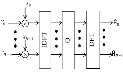
Figure 3: General Estimator Structure

2.2

PILOT AIDED CHANNEL

ESTIMATION

In pilot aided channel estimation scheme, pilot symbols are added at the transmitter side in which all subcarriers are used as pilots .If we assume that channel is constant then there will no channel estimation error since the pilots are sent at all carriers. The estimation can be performed by two methods. The first one is LS(Least Square) and the second one is MMSE(Minimum Mean Square Error).

2.2.1

LS Estimator

:

The first step in the channel estimation process is to remove the modulation of the pilot symbols. Thus, an initial estimate of the CTF (Channel Transfer Function) at pilot positions is obtained. The estimate of[12]channel transfer function is obtained by using LS estimator. The LS estimator for the cyclic impulse response h minimizes Υ-XFh)ᵸ Υ- XFh) and generates:

= F Fᵸ Xᵸ Y(3) Where,

=(Fᵸ XᵸXF

Note that also corresponds to the estimator structure

in Fig. 3. Since (3) reduces to: = Υ

The LS estimator is equivalent to what is also referred to as the zero-forcing estimator. Where(·)ᵸmeans the conjugate transpose operation Without using any knowledge of the statistics of the channels, the LS estimators are calculated with very low complexity, but they suffer from a high mean-square error. When the channel is slow fading, the channel estimation inside the block can be updated using the decision feedback equalizer at each sub-carrier.

2.2.2

MMSE Estimator

MMSE Estimator makes full use of the correlation of the channel frequency response at different times and frequencies. In particular, for mobile wireless channels, the correlation of the channel frequency response at different times and frequencies can be separated into the multiplication of the time and frequency domain correlation functions. Hence, MMSE channel estimator can be a frequency-domain filter using the fast Fourier transform (FFT), followed by timedomain filters. Since the channel statistics, which depend on the particular

environment, are usually unknown, we present a robust estimator, that is, an estimator that is not sensitive to the channel statistics. If the time domain channel vector h is Gaussian and un e ated with the hanne n ise ω, the frequency domain MMSE [12-13] estimate of h is given by:

=FRhY

Where,

ᵸ}=E{(F )ᵸ}=F Fᵸ ᵸ )ᵸ}= FᵸXᵸ

ᵸ}=XF FᵸXᵸ+

is the cross covariance matrix between h and yand

is the auto covariance matrix of Y. is the

autocovariance matrix ofH and represents the noise variance .

These two quantities abd are assumed to be

known. Since the columns in F are orthonormal,

generates the frequency-domain MMSE estimate by:

=F Fᵸ XᵸY (4)

where can be shown to be:

= [( Fᵸ XᵸXF + (Fᵸ XᵸXF

This MMSE channel estimator (4) has the form shown in Fig. 3.If h is not Gaussian, is not necessarily a minimum mean-square error estimator. It is however the best linear estimator in the mean-square error sense.The MMSE estimator yields much better performance than LS estimators especially under the low SNR scenarios. A major drawback of the MMSE estimator is its high computational complexity, especially if matrix inversions are needed each time the data in X changes.

2.2.3

LMS ITERATIVE CHANNEL

ESTIMATION

In this section, we propose a low-complexity ICE algorithm with improved error performance which employs the well known LMS algorithm.

Figure 4 :Implementing LMS Iterative alogirithm

It is given by:

= -1-hµ*X

Where,

 n = The iteration state  e = The signal error

 μ = A effi ient etween 0-1

As illustrated in figure 4.LMS algorithm is applied to receiver and the channel which was estimated in each iteration would be used for next iteration additionally the output signal is fed to source signal for next channel estimation. Another important factor in channel estimation through this method is µ which influences on estimation and should be precisely choosen. The performance of LMS algorithm can be closely to LS algorithm by careful choice of μ.

2.3

Estimator Complexity

The complexity of LMS iterative estimation is less than the conventional estimators. Notice that LS estimator has much lower complexity than MMSE estimator.

It should be noted that the MMSE estimators have been derived under the assumption of known channel correlation and noise variance. In practice these quantities,

and are either taken fixed or estimated, possibly in

an adaptive way. This will increase the estimator complexity and reduce the performance slightly.

Whereas in LMS iterative channel estimation, estimation in each iteration can be used as side information and feed back to system to achieve better result for next iteration. Thus this technique reduces the complexity and improves the performance.

3. SIMULATION AND EVALUATION

In this section we demonstrate the performance of proposed iterative channel estimation method for OFDM systems. In the simulation we consider an OFDM system operating with bandwidth of 8.75MHz,Length of FFT as 1024 and Guard Interval of 1/8.Total number of data bits are inserted uniformly at even and odd positions. System parameters used in the simulation are indicated in Table 1.

Table 1.OFDM system parameters

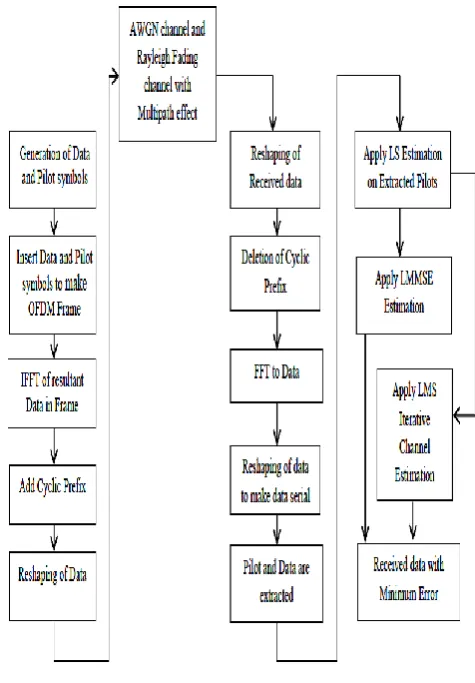
In the simulation we present 16 QAM modulation scheme. Total number of data bits taken are 1024 and 3456 OFDM symbols. The Flow Chart of the whole simulation process is as shown in the figure 5:

Figure 5: Flow Chart of Simulation Process

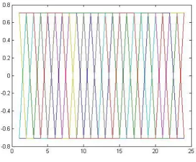
The generation of modulated OFDM data symbols is illustrated in figure 6:

Parameters Values

System bandwidth 8.75MHz

Sampling Frequency 10 KHz

Number of subcarriers 1024

Cyclic prefix 1/8

Modulation 16 QAM

Useful symbol Time 0.1024ms

OFDM Symbol Time 0.1152ms

Figure 6: Modulated OFDM data symbols

The equispaced pilot symbols and data are now constructed in the OFDM frame at even and odd positions. Pilot symbols can be viewed as shown in figure 7.

Figure 7: Pilot symbols representation

And data symbols can be viewed as,

Figure 8. Data symbols representation

Both Pilot symbols and data symbols constructed in OFDM frame is shown in figure 9:

Figure 9: Data and pilot representation in OFDM frame

The formation of OFDM frame can be seen as shown in figure 10:

Figure 10: Formation of OFDM frame

The next process in OFDM signal generation is taking the inverse fast fourier transform which converts the data in time domain. After that Cyclic Prefix is inserted which is responsible to avoid inter symbol interference. CP=1/8 is taken in the simulation process. In this paper 128 bits of cyclic prefix is inserted in OFDM frame..Finally we do reshaping of resultant data.

Table 2: BER Vs SNR for Different Channel Estimation Techniques

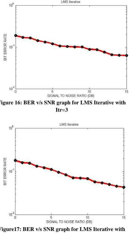
Table 2. shows the performance of different channel estimation methods between Bit Error Rate and Signal to Noise ratio.Table shows LMS iterative algorithm upto 4 iterations.

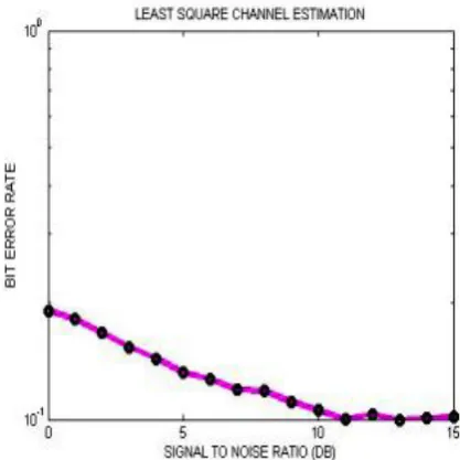
Following graphs shows the peformance of different channel estimation algorithms and which shows that LMS iterative algorithm performs better results than LS and LMMSE algorithms.

Figure 11: BER V/s SNR Graph for NO Channel Estimation

Figure 12: BER v/s SNR graph for Least Square SNR No

channel

LS MMSE BER(Bit Error Rate)

Itr=1 Itr=2 Itr=3 Itr=4 1 0.2255 0.1775 0.1935 0.1828 0.1779 0.17 0.16

2 0.2216 0.1624 0.1827 0.1668 0.162 0.1673 0.155

3 0.2193 0.1549 0.1765 0.1435 0.143 0.142 0.132

4 0.2096 0.1387 0.1665 0.1335 0.133 0.132 0.122

5 0.2053 0.1368 0.1629 0.1215 0.121 0.12 0.11

6 0.2044 0.1272 0.1617 0.1169 0.116 0.106 0.096

7 0.2031 0.1199 0.1563 0.1089 0.108 0.103 0.083

8 0.1994 0.1130 0.1509 0.1081 0.1071 0.101 0.071

9 0.1995 0.1099 0.1497 0.1008 0.103 0.1001 0.07

10 0.1968 0.1064 0.1476 0.0998 0.0898 0.088 0.068

11 0.1973 0.1063 0.1465 0.0991 0.0891 0.0871 0.0571

12 0.1945 0.1026 0.1426 0.0989 0.0859 0.0759 0.0545

13 0.1944 0.1007 0.1431 0.0893 0.0763 0.0653 0.0498

14 0.1926 0.1001 0.1393 0.0859 0.0739 0.0635 0.0455

Figure13: BER v/s SNR graph for LMMSE

Figure14: BER v/s SNR graph for LMS Iterative with Itr=1

Figure 15: BER v/s SNR graph for LMS Iterative with Itr=2

Figure 16: BER v/s SNR graph for LMS Iterative with Itr=3

Figure17: BER v/s SNR graph for LMS Iterative with Itr=4

4. CONCLUSION

5. REFERENCES

[1] IEEE Part II: Wireless LAN Medium Access Control (MAC) and Physical Layer (PHY) Specifications: High-Speed Physical Layer in 5 GHz Band. IEEE Sts. 802.11a-1999, 1999..

[2] J. S. Chow, J. C. Tu, and J. M. Cioffi.A discrete multitone transceiver system for HDSL application.IEEE J. Select. AreasCommun., 9:895– 908, Aug. 1991.

[3] Z. Wang and G. B. Giannakis.Wireless multicarrier communications where Fourier meets Shannon.IEEE Signal ProcessingMagazine, pages 29–48, May 2000. [4] P. H ehe , S. Kaise and I. R e ts n, “Two di mensional pilot-symbol-aided channel estimation by Wie er ilteri g,”i Proc. CASSP’97, pp.1845– 1848, April 1997.

[5] Coleri, S., Ergen, M., Puri, A., and Bahai, A., “Channel Estimation Techniques Based on Pilot Arra geme t i O M Systems,” ra sactio s on Broadcasting, vol. 48, pp. 223–229, Sept. 2002. [6] Y e. Li, “Pilot-symbol-aided channel estimation for

O M i wireless systems,” ra s. Ve . Technol., vol. 49, no. 4, pp. 1207-1215, 2000 [7] Ottersten, B., Viberg, M., and Kailath, T.,

“Performance Analysis of the Total Least Squares SPR Algorit m,” ra sactio s o Sig al Processing, vol. 39, pp. 1122–1135, May 1991. [8] H u, X., Li, S., Liu, D., in, C., and ue, G., “On

Two-dimensional Adaptive Channel Estimation in O M Systems,” 60t 9 EE Vehicular Technology Conference, Los Angeles, Ca., vol. 1, pp. 498–502, Sept. 2004.

[9] Sanzi, F., Sven, J., and S eide , J., “A Comparative Study of Iterative Channel Estimators for Mobile O M Systems,” ra sactio s o Wireless Communications, vol.2, pp. 849–859, Sept. 2003. [10] Li, ., “Simplified Channel Estimation for OFDM

Systems wit Multiple ra smit A te as,” Transactions on Communications, vol. 1, pp. 67-75, January 2002.

[11] J. J. van de Beek, O. Edfors, M. Sandell, S. K. Wi s n, and P.O. Bö jess n, “On channel estimation i O M systems,” i Proc. Ve icular Technology Conf., vol. 2, Chicago, IL, July 1995, pp. 815–819.

[12] Coleri, S., Ergen, M., Puri, A., and Bahai, A., “Channel Estimation Techniques Based on Pilot Arra geme t i O M Systems,” ra sactio s on Broadcasting, vol. 48, pp. 223–229, Sept. 2002. [13] Louis L. Scharf, Statistical Signal Processzng,

Addison-Wesley, 1991

[14] Chen, J., C. Chiang and L. Lo, 2007. Iterative Channel Estimation for MIMO OFDM Systems. Proceeding of the International Symposium on Intelligent Signal Processing and Communication Systems, Nov. 28-Dec. 1, IEEE Xplore Press,

Xiamen, pp: 774-777. DOI:

10.1109/ISPACS.2007.4446002.

[15] Qiao, Y., S. Yu, P. Su and L. Zhang, 2005. Research on an iterative algorithm of LS channel estimation in MIMO OFDM systems. IEEE Trans. Broadcast.,51: 149-153. DOI: 10.1109/TBC.2004.842524

AUTHOR’S PROFILE

Rajeshwar singhis M.Tech. student in the Department of Electronics and communication at Lovely Professional University Phagwara,Punjab.He received his B.Tech. from same University in September 2011.He has worked as an engineer in Airtel Telecom for 6 months. His research interests include communication theory and Ad-hocnetworks.