Optimized Proposed Algorithm for Graph Traversal
Ankit Malhotra
B.TECH(IT) Information Technology
Department ASET,Delhi, India
Dipit Malhotra
B.TECH(IT) Information Technology
Department MSIT,Delhi,India
Saksham Kashyap
B.TECH(IT) Information Technology
Department MSIT,Delhi,India
ABSTRACT
This paper includes a flexible algorithm for traversing a directed and an undirected graph. Graph traversal is defined as the problem of visiting all the nodes in a graph in a particular manner, updating and/or checking their values along the way. The Breadth first search along with Depth first search are the most widely used algorithms for traversing a graph. In this article, an algorithm is proposed for traversing a graph taking in consideration the vertex with the maximum outgoing edges. Instead of beginning from the root node and then gaining access to visit the neighbors of the currently visited node, the algorithms looks for the vertex with the maximum edges and then continue traversing all the neighboring vertices of that vertex. This paper presents an algorithm to traverse an undirected or a directed graph and calculates the time and space complexity of the algorithm. The work proposed here intends to find a new algorithm that can be universally applied to all types of graphs
General Terms
Your general terms must be any term which can be used for general classification of the submitted material such as Pattern Recognition, Security, Algorithms.
Keywords
Keywords are your own designated keywords which can be used for easy location of the manuscript using any search engines.
1.
INTRODUCTION
Graphs are the commonly used data structures that describe a set of objects as nodes and the connections between them as edges. A large number of graph operations are present, such as Bellman ford minimum spanning tree, breadth-first search, shortest path etc., having applications in different problem domains like data mining[1], and network analysis[2], route finding[3] , game theory[4].
With the development of computer and information system, the research on graph algorithm is wide opened. The two most widely used algorithms used for traversing a graph are Breadth First Search and Depth First Search [5]. The BFS begins at a root node and inspects all the neighbouring nodes. Then for each of those neighbour nodes in turn, it inspects their neighbour nodes which were unvisited[6], and so on , while the DFS remove a vertex from a container , prints it and finds all the adjacent vertices . On finding the adjacent vertices it marks them visited and enter them into a stack. The algorithm is repeated as long as the stack is not empty. So far, many different variants of BFS and DFS algorithm have been implemented sequentially as well as in parallel manner. In all parallel implementations, the unvisited nodes of the root node are visited, but in our implementation, the node
with the maximum number of edges if processed first and then its neighboring nodes are processed.
This paper presents a new algorithm for traversing a graph and then compare the traversal result of a directed and undirected graph using BFS , DFS and the new algorithm. The traversal path obtained by employing all the techniques is shown and then a comparison of the time and space complexity of all the algorithms is done.
The rest of the paper is organized as follows: Understanding graph traversal is done in section 2. Graph traversal by the proposed algorithm is discussed in Section 3. Section 4 presents a traversal of a directed graph using BFS, DFS and the proposed algorithm. Performance analysis of the proposed algorithm with BFS and DFS is done in section 5.Future Scope is discussed in section 6 and finally concluded in section 7.
2.
BASIC CONCEPT OF GRAPH
TRAVERSAL
The goal of a graph traversal, generally, is to find all nodes reachable from a given set of root nodes. To traverse a graph is to process every node in the graph exactly once.
2.1
Graph Representations
Different data structures for the representation of graphs are used in practice [7]:
Adjacency list
: In graph theory and computer science, an adjacency list describes the set of neighbors of the vertex of a graph as a collection of unordered list. Each vertex has been associated with an unordered list. For example if a vertex B is connected to nodes C and D with an outgoing edge from B to C and from B to D as show in figure 1 , then the adjacency list representation will be ::Adjacency List:
B: C , D
C : -
D: -
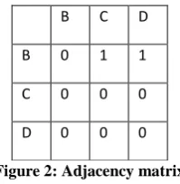
Adjacency Matrix: The adjacency matrix is a matrix with rows and columns labeled by graph vertices, with a 1 or 0 in
position according to weather and
and vj. In the adjacency matrix , 1 denotes that a path exists between the two nodes while 0 denotes that no path exists between the two nodes .The concept of adjacency matrix can be employed onto the graph in figure 1 .The adjacency matrix for the graph in figure 1 is:
[image:2.595.117.217.131.233.2]B C D B 0 1 1 C 0 0 0 D 0 0 0
Figure 2: Adjacency matrix
Incidence Matrix : An incidence matrix is a two-dimensional Boolean matrix, in which the rows represent the vertices and columns represent the edges. The entries indicate whether the vertex at a row is incident to the edge at a column.
Incidence matrix of the graph in figure 1 is:
b 1
1
c 1
0
d 0
0
Figure 3: Incidence matrix of graph
2.2
Graph Traversal Algorithms
The most widely used algorithms for traversing a graph are: 1. Breadth First Search: Ingraph theory,
breadth-first search(BFS) is astrategy for searching in a graphwhen search is limited to essentially two operations: (a) visit and inspect a node of a graph; (b) gain access to visit the nodes that neighbour the currently visited node. The BFS begins at a root node and inspects all the neighbouring nodes. Then for each of those neighbour nodes in turn, it inspects their neighbour nodes which were unvisited, and so on.
Algorithm for Breadth First Search (BFS) [8]
Figure 4: Breadth First Search Algorithm
2. Depth First Search: It is an algorithm for traversing a graph in which one starts at the root and explores as far as possible along each branch before backtracking. Formally, DFS is an uninformed search that progresses by expanding the first child node of the search tree that appears and thus going deeper and deeper until a goal node is found, or until it hits a node that has no children. Then the search backtracks, returning to the most recent node it hasn't finished exploring. In a non-recursive implementation, all freshly expanded nodes are added to a stack for exploration.
Algorithm for Depth First Search [9]
The algorithm uses a stack data structure to store intermediate result as it traverses the graph as follows:
3.
TRAVERSAL OF GRAPH BY
[image:2.595.67.190.309.374.2]PROPOSED ALGORITHM
Figure 5: Undirected graph
Consider the above graph. The algorithm for traversing the graph is as follows:
The adjacency matrix of the graph along with an array SUM that corresponds to the summation of the edge count of different nodes is given.
Starting node: A Step 1:
Initially, construct an adjacency matrix of graph along with the SUM array.
Adjacency Matrix SUM
A B C D E F G A 0 1 1 0 1 0 0 B 1 0 0 1 0 0 1 C 1 0 0 1 1 1 0 D 0 1 1 0 0 0 1 E 1 0 1 0 0 1 0 F 0 0 1 0 1 0 1 G 0 1 0 1 0 1 0
3 3 4 3 3 3 3
1. First remove a vertex from a stack and print it. 2. Find all adjacent vertices of that node and mark them as visited.
Initially the visited array will be:
Step 2: After going to A, it’s neighboring unvisited nodes(B,C,E) gets visited and thus the adjacent edge count for A,B, C and E will be 0
Adjacency matrix SUM
The visited array will become:
Step 3:
Now the node with the maximum edge count is the Sum array is 2.So one can take B, C or G.
Taking B, after B is processed, it’s neighboring unvisited nodes (D and G) gets visited and the edge count for B, D and G will be 0.
Adjacency matrix Sum
The visited array will be:
Step 4:
Now the node with the maximum edge count is the Sum array is 1 .So one can take either C, E or G.
Consider C and after node C is processed, it’s neighboring unvisited node (F) gets visited and the edge count for F will be 0.
Adjacency Matrix SUM
The visited array will be:
A B C E D G F
As all the nodes get visited, the proposed algorithm traverses the graph. The order of traversal is A , B , C , E , D , G , F
4.
COMPARISON OF BFS AND DFS
WITH PROPOSED ALGORITHM
In this section, a comparison between general traversal algorithms and proposed algorithm is done. The traversal techniques will be implemented on the same graph to identify and compare the path taken by each one of them.
Figure 10: Directed graph
Let us consider the above graph. The adjacency list for the above Graph is
Figure 11:Adjacency list
null Null null null null null Null
0
2
2
1
1
1
2 A B C D E F G
A 0 0 0 0 0 0 0
B 0 0 0 1 0 0 1
C 0 0 0 1 0 1 0
D 0 0 0 0 0 0 1
E 0 0 0 0 0 1 0
F 0 0 0 0 0 0 1
G 0 0 0 1 0 1 0
A B C E null null Null
A B C D E F G
A 0 0 0 0 0 0 0
B 0 0 0 0 0 0 0
C 0 0 0 0 0 1 0
D 0 0 0 0 0 0 0
E 0 0 0 0 0 1 0
F 0 0 0 0 0 0 0
G 0 0 0 0 0 1 0
0
0
1
0
1
0
1
A B C E D G null
A B C D E F G
A 0 0 0 0 0 0 0
B 0 0 0 0 0 0 0
C 0 0 0 0 0 0 0
D 0 0 0 0 0 0 0
E 0 0 0 0 0 0 0
F 0 0 0 0 0 0 0
G 0 0 0 0 0 0 0
0
0
0
0
0
0
0
Graph Traversal using BFS:
a) Initially add A to the Queue and add NULL to ORIGIN.
Front = 1 Queue = A
Rear = 1 Origin=null
b) Remove the front element A from the Queue by setting Front = Front+1 and add to the Queue the neighbours of A.
Front = 2 Queue = A, B, D
Rear = 3 Origin = null, A, A
c) Remove the front element B from the Queue by setting Front = Front+1 and add to the Queue the neighbours of B.
Front = 3 Queue = A, B, D, F Rear = 4 Origin = null, A, A, B d) Remove the front element D from the Queue
by setting Front = Front+1 and add to the Queue the neighbours of D.
Rear = 5 Origin = null, A ,A, B , D Front = 4 Queue = A, B, D , F,E a) Now the last node C gets traversed at the end.
Front = 4 Queue = A, B, D , F ,E Rear = 5 Origin = null, A ,A, B , B So the final traversed order of the graph is :
A , B , D , F , E , C
Graph traversal using DFS :
Let us consider the above graph. First create the traversed at the adjacency list of the graph and then apply the traversal algorithm.
The adjacency list of the graph is : .
Considering the above graph and Adjacency list.
The traversal of the graph using Depth First Search takes place in the following:
a) Initially push A onto the Stack. Stack : A
b) Pop and print A , and push onto the Stack all the neighbours of A
Stack : B , D Print : A
c) Pop and print D & push onto stack all the neighbors of D
Stack: B, E Print: D
d) Pop and print E,and push onto stack all the neighbors. Since E has no neighbors nothing will be pushed onto the stack.
Stack: B Print : E
e) Pop and print B & push onto stack all the neighbours of B Stack : F Print : B
f) Pop and print F, and push onto stack the neighbours of F. Since F has no neighbours, stack remains empty Stack: - Print: F g) Now the last node C gets traversed.
Stack: - Print: C
Now since the stack is empty, all the nodes of the graph have been traversed.
The order of traversal is: A, B, F, D, E, C.
Now that the traversal path using both DFS and BFS as been obtained. The same graph will now be traversed using proposed algorithm.
Graph traversal using Proposed Algorithm:
Let us consider the above graph. First create the an adjacency matrix along with a matrix sum .
The sum matrix is the summation of the edge count of each
row of the adjacency matrix.. Let us consider the same graph. The adjacency matrix
for the graph is :
Adjacency Matrix SUM
.
A B C D E F A 0 1 0 1 0 0 B 0 0 0 0 0 1 C 0 0 0 0 1 1 D 0 0 0 0 1 0 E 0 0 0 0 0 0 F 0 0 0 0 0 0
2 1 2 1 0 0 Adjacency List
The visited array will be empty.
Step 1: Initially start the traversal from the starting node A.
Step 2
:
After going to A, it’s neighboring unvisited nodes (B,D) gets visited and thus the adjacent edge count for A,B, and D will be 0.So the adjacency matrix will be:
Adjacency Matrix
Sum
The visited array becomes
Step 3: Now the node with the maximum edge count in the sum array is 2. Consider node C, and after C is processed, its neighbouring unvisited node (E & F) gets visited and thus the edge count for C,E will be 0.
So the adjacency matrix will be
Adjacency matrix SUM
The visited array becomes
Step 4: As all the nodes get visited, the proposed algorithm traverses the graph. The order of traversal is A , B , D , C , E , F
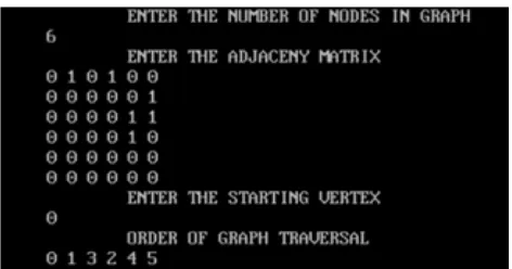
[image:5.595.316.552.182.306.2]The traversal of this graph using a C program:
Figure 12 : C program output showing the order of traversal
5.
PERFORMANCE ANALYSIS:
Algorithm Time Complexity Space Complexity Breadth First
Search(BFS) Depth First Search (DFS) Proposed algorithm
[image:5.595.310.547.355.524.2](In worst case only)
Figure 13: Comparison on the basis of time & space
complexity[10] .
Best and average Case analysis of Proposed Algorithm: [1] Applications of graph theory in communication networks by Suman Deswal
If the graph is not weighted, and therefore all step costs are equal, the proposed algorithm will find the nearest and the best solution.
If the shallowest goal node is at some finite depth say d, the proposed algorithm will eventually find it after expanding all shallower nodes .
In the best and average case, the proposed algorithm will not consider each and every edge to traverse the graph and thus the Time complexity will be less as compared to BFS or DFS.
Worst case analysis of Proposed Algorithm:
If the graph is infinite and there is no solution the algorithm will diverge.
In the worst case, the time complexity is similar to Breadth First Search(BFS) i.e. the proposed algorithm has to consider all paths to all possible nodes .So the time complexity will
Null Null Null Null Null Null
A B C D E F
A 0 0 0 0 0 0 B 0 0 0 0 1 0 C 0 0 0 0 1 1 D 0 0 0 0 0 1 E 0 0 0 0 0 1 F 0 0 0 0 0 0
0 1 2 1 1 0
A B D null null Null
A
B
C
D
E
F
A
0
0
0
0
0
0
B
0
0
0
0
0
0
C
0
0
0
0
0
0
D
0
0
0
0
0
0
E
0
0
0
0
0
0
F
0
0
0
0
0
0
0
0
0
0
0
0
be
which is O(bd). The time complexity can also be expressed as O ( | E | + | V | ) since every vertex and every edge will be explored in the worst case.
6.
Future Scope
The proposed algorithm can be further be improved in terms of running time and space. The time complexity is same in the worst case when the algorithm traverses each vertex along each path. The algorithm sometimes cannot traverse the graph accurately. In case of directed graph the proposed algorithm sometime fails to traverse it accurately similar to BFS and DFS. However, the proposed algorithm has a time complexity much less than BFS or DFS when it does not have to go through each edge to traverse the nodes. This also reduces the space complexity as well. However, the accuracy can still be improved. The algorithm can still be made time and space efficient.
7.
REFERENCES
[1] Applications of graph theory in communication networks by Suman Deswal.
[2] Shortest path algorithm in GIS network analysis based on Clifford algebra by Jiyi Zhang, Weichang, Mei, Wen Luo, Linwang Yuan.
[3] Graph theory and applications by Paul Van Dooren [4] Applications of graph theory by S.G.Shirinivas
S.Vetrivel , Dr.N.M. Elango
[5] BFS by Allison June Barlow Chaney,Princeton.edu. [6] DFS by Allison June Barlow Chaney.
[7] Introduction to Algorithms(2nd ed) by Cormen Thomas H, Leiserson , Charles E,Clifford(2001)
[8] Breadth First Search WIKIPEDIA [9] CMU-Data Structures Lessons 5
[10]Graphs :Representation and Exploration by Julian Mestre [11]Y.T. Yu, M.F. Lau, "A comparison of MC/DC, MUMCUT and several other coverage criteria for logical decisions", Journal of Systems and Software, 2005, in press.