Munich Personal RePEc Archive
Spatial design matrices and associated
quadratic forms: structure and
properties
Hillier, Grant and Martellosio, Federico
University of Southampton
2006
Online at
https://mpra.ub.uni-muenchen.de/15807/
www.elsevier.com/locate/jmva
Spatial design matrices and associated quadratic
forms: structure and properties
Grant Hillier
∗, Federico Martellosio
Division of Economics, School of Social Sciences, University of Southampton, Highfield, Southampton, SO17 1BJ, UK
Received 1 May 2003 Available online 7 January 2005
Abstract
The paper provides significant simplifications and extensions of results obtained by Gorsich, Gen-ton, and Strang (J. Multivariate Anal. 80 (2002) 138) on the structure of spatial design matrices. These are the matrices implicitly defined by quadratic forms that arise naturally in modelling intrinsically stationary and isotropic spatial processes. We give concise structural formulae for these matrices, and simple generating functions for them. The generating functions provide formulae for the cumulants of the quadratic forms of interest when the process is Gaussian, second-order stationary and isotropic. We use these to study the statistical properties of the associated quadratic forms, in particular those of the classical variogram estimator, under several assumptions about the actual variogram. © 2004 Elsevier Inc. All rights reserved.
AMS 1991 subject classification:Primary: 62H11; Secondary: 62H10
Keywords:Cumulant; Intrinsically stationary process; Kronecker product; Quadratic form; Spatial design matrix; Variogram
1. Introduction
In modelling spatial data—in general ind dimensions—observed at sites labelled by points in some subset ofRd, it is often assumed that the process is intrinsically stationary and isotropic (see below and[6]). Such models are then—intuitively at least—generalizations
∗Corresponding author.
E-mail addresses:[email protected](G. Hillier),[email protected](F. Martellosio).
G. Hillier, F. Martellosio / Journal of Multivariate Analysis 97 (2006) 1 – 18
of familiar stationary time series models defined on the line (the cased =1), and, we shall see that there is quite a formal structure that reflects this relationship (Theorem1below).
In this paper, as in the recent paper by Gorsich et al.[10](hereafter abbreviated to GGS), we assume that the observational sites are located on a uniform grid inRd, withnsites on each ofdaxes. Sites may then be labelled by elements of the set=(n, d)of sequences
=((1), . . . ,(d))of non-negative integers satisfying 0(i)(n−1)fori=1, . . . , d, and, to avoid ambiguity, we order the sequences inlexicographically. Extensions to the case of a rectangular grid are straightforward, but for simplicity we confine our results to the hypercubic grid.
Denoting the observed process by{Z(); ∈ }, intrinsic stationarity entails the
as-sumptions thatE(Z())is constant, and that, for = ,(,) = V ar(Z()−Z())
depends on(,)only through(−), and the isotropy assumption that(,)depends
on(,)only throughh= −2, the squared Euclidean distance between the sites
and. In that case the function 2(h)defined by
2(h)=V ar(Z()−Z()) (1)
is called thevariogramof the processZ(). Note that, here and throughout, we usehto denote thesquared Euclidean distance −2 = d
i=1((i)−(i))2 between sites, rather than (as is more common)−itself. This is notationally more convenient later. Henceforth we takehto be strictly positive unless otherwise indicated.
The natural estimator for 2(h)is based on the function
qh=
N (h)
(z()−z())2, (2)
wherez()denotes the observed value ofZ(), andN (h)is the set of (unordered) pairs
(,)satisfying−2=h. Note that both(0)=0 andq0=0. Statistics of this form are also of interest more generally in the context of modelling spatial processes.
Forh >0 the expression on the right in (2) may be written as a quadratic form
qh=z′Lhz=z′(Dh−Ah)z, (3)
wherez=(z();∈)denotes theN-dimensional vector of observations,LhandAhare
symmetric, andDhis a diagonal matrix. Here and throughoutN =nd= ||, the cardinality
of, denotes the total sample size. The matrix of this quadratic form,Lh, is theN×N
spatial design matrixat distance√h, andDhand−Ahare, respectively, the diagonal and
off-diagonal parts ofLh. By expanding the right side of (2) it is easy to see thatAh has
a one in positions labelled by pairs(,)satisfying−2 =h, and zeros elsewhere, and that the diagonal element in rowofDhis the number of sequences∈satisfying
−2=h, i.e., the sum of the elements in rowofAh. The matricesLh =Lh(n, d)
in (3) are, in GGS, denoted byA(d)(nd, h), with h = −. The matrixAh may be
interpreted as the adjacency matrix of a graphG(, h)with vertex setand edges the pairs
(,)∈×for which−2=h. In that contextLhis known as the Laplacian matrix
As already mentioned, an important application of the quadratic formsqhis to the
esti-mation of the variogram in geostatistics. LetNh = |N (h)|denote the cardinality of the set
N (h). The statistic 2ˆ(h)=qh/Nh, is an unbiased estimator of 2(h), and is often referred
to as the classical variogram estimator (see Section 3.2 below, and GGS and the references therein). However, for other purposes it is also of interest to consider the statistics
qh∗=2
N (h)
z()z()=z′Ahz, (4)
based on just the off-diagonal part ofLh. To give just a few examples: (i) the statisticqh∗,
normalized byz′z, is used to test for spatial autocorrelation at distance√h(see[18]); (ii) if the covariance matrix of the process belongs to the linear span of (some of) the matrices
Ah, that is, if the spatial process is not only intrinsically stationary and isotropic, but also
second-order stationary, the statisticqh∗/(2Nh) is (when the process has zero mean) an
unbiased estimator of the covariance function at distance√h(see Section 3.2); (iii) if the process is assumed to be Gaussian with precision matrix (inverse covariance matrix) that is a linear combination of matricesINand{Ah,h∈Hp}, whereHpcontainspdistinct values
ofhandINdenotes theN×Nidentity matrix, then apth order conditional autoregression
is obtained[4]. The matricesAh,h∈Hp, play the role of spatial weights matrices, and the
quadratic forms(z′z, qh∗, h ∈ Hp), are minimal sufficient statistics for the parameters of
the model, and thus form the basis for inference on those parameters.
The problem of interest here is to give structural formulae for the matricesAh, and
thereby forDh andLh. Thus, we continue the work of GGS, whose aim was to analyze
the eigenstructure of the matricesLh, with a view to deducing the properties of statistics
likeqhandqh∗, or more specifically of the variogram estimator 2ˆ(h). It is well-known that
under Gaussian assumptions (and also more generally) the properties ofqhandqh∗depend
uponLhandAh, respectively, only through their eigenvalues. Our purpose in the present
paper will be to simplify and extend the results given in GGS.
In Section 2, we first provide a complete structural representation of the matricesAhand
Lh, and then give generating functions that make their computation straightforward with a
standard symbolic computation package. In principle this completely solves the eigenvalue problem, but in practice, sinceNis usually quite large, direct computation of the eigenvalues would be unreliable. And, as we shall see, except in special cases, bothAhandLhare sums
of non-commuting matrices. Since, in this case, it is generally not possible to express the eigenvalues of the sum in terms of those of the summands, general explicit formulae for the eigenvalues are unlikely to be accessible.
Fortunately, our generating function results do permit the computation of the cumulants of the statistics of interest very simply and directly. In Section 3, we use these expressions to study the properties of the statisticsqh andqh∗ under the assumption that the process
G. Hillier, F. Martellosio / Journal of Multivariate Analysis 97 (2006) 1 – 18
2. The matricesAh,Dh andLh
In this section we give the main structural results for the matricesAh,DhandLh. The
elements of these matrices, indexed by pairs(,)∈ ×, are completely determined byn,dandh. The results express these matrices ind >1 dimensions in terms of sums of Kronecker products of the corresponding matrices in dimensiond =1. We begin with the key result—a very simple structural formula for the matricesAh.
2.1. Off-diagonal part
The matricesAhare defined by
(Ah),=
1 if −2=h,
0 otherwise. (5)
Evidently, settingA0=IN,h0Ah=JN, whereJqis theq×qmatrix with all elements
one. In dimensiond =1 we denote then×nmatricesAr2 byFr,r = 0,1, . . . , n−1.
That is,
(Fr)i,j =
1 if|i−j| =r,
0 otherwise. (6)
Sincen−1
r=0Fr =Jn, we have that
JN = d
1
Jn = d
1 n−1
r=0
Fr
=
∈
(F(1)⊗F(2)⊗ · · · ⊗F(d)) (7)
by the multilinearity of the Kronecker (or direct) product ‘⊗’. Note that the elements of
F⊗=F(1)⊗F(2)⊗ · · · ⊗F(d) (8)
are zeros and ones, soexactly one termF⊗on the right in (7) has a one in any given position
(,). In view of (7), the following result is not surprising:
Proposition 1. Leth= {∈: 2=h}.Then:
Ah =
∈h
F⊗. (9)
Proof. For each pair(,)∈×, define∈by(i)= |(i)−(i)|, i=1, . . . , d. From the definition ofAh,(Ah), =1 if and only if2=h, or∈ h. On the other
hand, the(,)element of(F(1)⊗F(2)⊗ · · · ⊗F(d))is one if and only if
|(i)−(i)| =(i), f or i=1, . . . , d. (10)
For example, ifh = 1,1consists ofd sequences containing a single one andd−1 zeros, so that
A1=
d
i=1
(In⊗ · · · ⊗F1⊗ · · · ⊗In)
withF1in theith position in theith term (see the discussion of Eq. (9) in GGS). Likewise, forh=2,2consists of the(d2)sequences that contain 2 ones andd−2 zeros, so in the corresponding expression forA2each term in the sum containsF1twice. Notice that, in both of these low-order cases, all the sequences that appear inh are permutations of a
single sequence.
An alternative proof of Proposition1based on known graph-theoretic results is worth recording, because it shows immediately how to generalize the result to cover index sets more complex than the uniform grid, e.g., the rectangular grid mentioned in the Introduction. We refer the reader to Cvetkovi´c et al.[7]for more on the graph-theoretic details.
Given graphsGi(Vi, Ei),i=1, . . . , d, with vertex setsVi and edge setsEi, thedirect
productof theGi,G1× · · · ×Gd is the graphG×d, say, defined as follows. The vertex
set ofG×d is the Cartesian productVd× =V1× · · · ×Vd of theVi, and ifxi, yi ∈ Vi for
i=1, . . . , d,(x1, . . . , xd)and(y1, . . . , yd)are adjacent inG×d if and only if(xi, yi)∈Ei
fori=1, . . . , d. In our case, the matricesFr, r =0, . . . , n−1, are the adjacency matrices
of the (so-called distance) graphsGr with common vertex setsVr =V = {0, . . . , n−1},
and with edge sets defined by: fori, j ∈ {0, . . . , n−1},(i, j )∈Eronly when|i−j| =r.
Then,Vd× = , and for each ∈we may define a productG×d()of the graphsG(i)
as above. It is known thatG×d()has adjacency matrixF⊗(Cvetkovi´c et al.[7, Theorem 2.21]). Thus, for any subsetUof, the union of the graphsG×d()has adjacency matrix
AU =∈UF⊗. Proposition1gives the caseU=h.
Call two sequences(,) h-neighborsif the sequence defined in (10) is inh. This
definition of neighbors—based on the Euclidean distance between points—is natural in
some contexts, but in others a neighborhood structure based, say, on theL1-norm (the
length of the shortest walk connectingto) may be more appropriate. The observation in the previous paragraph makes it straightforward to extend the results to follow to this case (and to neighborhood structures defined by otherLp-norms), but we omit the details.
2.2. Diagonal part
The matricesDhin (3) are diagonal matrices with diagonal elementsDh()equal to the
number ofh-neighborsof. In dimensiond = 1 define, for eachr = 0, . . . , n−1, the diagonal matrixMr withith diagonal element theith row sum ofFr, and then define, for
∈,
M⊗=M(1)⊗M(2)⊗ · · · ⊗M(d). (11)
It is straightforward to prove:
Proposition 2. Dh =∈hM
G. Hillier, F. Martellosio / Journal of Multivariate Analysis 97 (2006) 1 – 18
Notice thatt r[Dh]is the total number of non-zero elements inAh, so thatt r[Dh] =2Nh.
We have now established:
Theorem 1. The spatial design matrix at distance√his given by
Lh=
∈h
(M⊗−F⊗), (12)
whereM⊗andF⊗are as defined in(11)and(8).
The above expressions for the matricesAh,Dh, andLh involve summing over the set
h. We next examine this set more closely, and give formulae for these matrices that do not
involveh.
2.3. Generating functions
Sincehmust be a sum of squares ofdof the integers(0,1, . . . , n−1), not all values of
hd(n−1)2are feasible. This is so even whend4, notwithstanding Lagrange’s four-square theorem[11, Section 20.5], because no term in the decomposition ofhcan exceed
(n−1)2. Thus,hin Proposition1can be empty, and in that case we defineAh, Dhand
Lhto be zero matrices.
The values ofhthat yield non-vanishing matricesLhcan be read off from the expansion
of the polynomial
(1+t+t4+ · · · +tr2 + · · · +t(n−1)2)d=
d(n−1)2
h=0
mhth, (13)
in which the coefficientmhis evidently the number of ways in whichhcan be expressed
as a sum of squares ofdof the integers(0,1, . . . , n−1), i.e.,mh = |h|is the number of
h-neighbors of the origin. Except for the restrictionhd(n−1)2, themhevidently depend
ondbut not directly onn. Lettingfn(t )=nr=−01tr
2
, and using Wilf’s[20]notation, we may write
mh= [th](fn(t ))d, (14)
where[th]means “the coefficient ofthin the expansion of the following function in powers oft”. Note that[th]is identical to the operator(h!)−1(*/*t )h|
t=0, and, as an operator, is therefore linear. A cumbersome formula for themhcan be deduced from (14), but using a
modern symbolic computing package it is a simple matter to computemhfrom (14) without
having to rely on such formulae. Similarly, lettingbn(t )=nr=−10tr
2
xr, where thexiare labels for the integers 0,1, . . . , n−
1, obeying the usual rules of multiplication, we see that, from the formal expansion of
(bn(t ))d,
[th](bn(t ))d =
∈h
d
i=1
Thus, the sequencebelongs tohonly if the productdi=1x(i)appears on the right in
(15).
The key to obtaining a simple representation for the matricesAh,Dh, and henceLh, is
to notice that the scalar generating function(bn(t ))dcan be generalized in such a way that,
when expanded, the coefficient ofthis preciselyAh. To see this, define the matrix
Bn(t )= n−1
r=0
tr2Fr, (16)
ann×nToeplitz matrix with(i, j )elementt(i−j )2. By direct expansion of thedth Kronecker powerBn⊗(t ) =d
1Bn(t ), it is clear thatAh is the coefficient ofth in the expansion of
Bn⊗(t )in powers oft. That is,
Ah = [th]Bn⊗(t ). (17)
Similarly, letting
Cn(t )= n−1
r=0
tr2Mr (18)
andCn⊗(t )=d
1Cn(t ), we see that
Dh = [th]Cn⊗(t ). (19)
We therefore have the simple generating-function representation forLhgiven in:
Theorem 2. The spatial design matrix at distance√his given by
Lh= [th](Cn⊗(t )−Bn⊗(t )). (20)
These results evidently do not require knowledge ofh: it is built in to the generating
function. On the other hand, the matrices appearing in these representations ofAh,Dhand
LhareN×N, and likely to be high-dimensional, so it might seem that these results would
be of little practical value. On the contrary, we will see in the next section that they provide both analytically and computationally convenient information about the statisticsqh and
qh∗discussed in the Introduction, and hence about the properties of the variogram estimator 2ˆ(h). Before doing so we note some further implications of these results.
It is clear that, if∈h, so is every permutation of the elements of. Thus,hmust be
a union of one or more orbits inunder the action of the symmetric groupSd(the group of
permutations ofdobjects). A set of orbit representatives is provided by the set=(d, n)
ofnon-decreasingsequences=((1), . . . ,(d))∈, with(1)(2)· · ·(d). Leth = {∈ : 2=h}, and, forj =0, . . . , n−1, ∈ , letk(j )denote the
multiplicity ofjin, so thatn−1
j=0k(j )=d, and write ()=nj−=10 k(j )!, with, as
G. Hillier, F. Martellosio / Journal of Multivariate Analysis 97 (2006) 1 – 18
With this notation it is easy to see thatmh=d!∈h( ())
−1, and since
h= {:
∈h,∈Sd}, wheredenotes the permutationof, we have that
Ah =
∈h 1
()F
∗ ,
whereF∗ =
∈SdF
⊗
is a symmetric function of the matricesF(1), . . . , F(d). By an
obvious extension of this argument to the off-diagonal part, and settingM∗ =
∈Sd M⊗ , we can state:
Theorem 3. The spatial design matrix at distance√his given by
Lh=
∈h 1
()(M
∗
−F∗). (21)
For many values ofhEq. (15) reveals thathconsists of a single orbit, which is to say
thathhas a single element, sayh. In that casemh=d!/ (h), and Theorem3gives the
very simple result thatLh =( (h))−1(M∗h−F ∗
h). In the example following Proposition
1, for instance,h=1,1=(0, ..,0,1)and (1)=(d−1)!.
Using these results we may also obtain the following generalization and simplification of Lemma 6.1 and Theorem 6.1 in GGS, which give upper bounds on the largest eigenvalues ofLhandAh(for setshwith low cardinality), and hence upper bounds for the normalized
statisticsz′Lhz/z′zandz′Ahz/z′z.
Lemma 1. Lethandhdenote the largest eigenvalues ofAhandLh,respectively,and
letuh=d!∈h 2d−k(0)
() .Thenhuhandh2uh.
Proof. Let gh = max∈ Dh() denote the maximum number ofh-neighbors for any
point in the grid. The numbermh is the number ofh-neighbors of the origin, so that
ghmh. Under the condition that no sequence ∈ h contains an element(i) > n/2,
we havegh =uh. To see this, suppose first thath contains just the single sequenceh.
Ifkh(0)=0,gh =2
dm
hbecause, under the stated condition, max∈Dh()occurs at a
sequencefor which theh-neighbors in all 2ddirections enterD
h(), andmhcounts just
theh-neighborsin the direction for which the vector−has only positive components. Ifkh(0) > 0, only 2
d−kh(0) distinct directions are needed. Repeating the argument for each∈hproves the claimgh=uh. Finally, when the condition that no(i)exceedsn/2
is dropped, it is clear thatghuh. The assertionshuh,h2uhfollow by Gershgorin’s
theorem (see[16]).
Ifhcontains only the single sequenceh, which contains only one non-zero term (soh
contains only what GGS call “non-diagonal directions”), the matrices in the sum ∈hF
⊗
arepairwise commutative, so the eigenvalues ofAh are simple functions of those of the
single matrixFr (r =
√
h)involved. Under the same condition,Lh =((d−1)!)−1L∗h,
withL∗ h=
∈SdL
⊗
GGS note in Lemma 5.1, in the case of non-diagonal directions the eigenvalues ofLhare
simple functions of those of the matrix(M√
h−F√h).
The necessary and sufficient conditions required to ensure pairwise commutativity of the summands in Theorem 3 are thathcontains only the single sequenceh, andhcontains
no more than one (possibly repeated) non-zero integer. Note thath may correspond to
what GGS would call “diagonal directions”, and that these conditions are always satisfied forh=1,2,3 (for anydh), but otherwise clearly hold only for special values ofh.
3. Applications
In this section, we use the results established above to study the properties of the statistics
qh∗=z′Ahzandqh=z′Lhz. We consider first the case in whichz∼N (0, IN), but in Section
3.2 show how our earlier results can be used to deal with the more general casez∼N (0,), assuming the process is second-order stationary and isotropic.
3.1. Properties of the quadratic formsqh∗andqh
Under the assumptionz∼N (0, I ), the distributions of the quadratic formq =z′Az, and its normalized formq¯ =z′Az/z′z, can certainly be obtained (see[14]for the former, and
[13]for the latter), but both are sufficiently complicated as to inhibit their use for practical study of, and/or tabulation of, the distribution. On the other hand, it is well known that the cumulants ofq =z′Azunder the assumptionz∼N (0,)are given by
p=2p−1(p−1)!t r[(A)p], p=1,2, . . . (22)
(see[15]Chapter 3 for the definition of cumulants, and Chapter 15 for the result given in Eq. (22)). The results in Section 2 allow these cumulants to be computed quite straightforwardly when=IN and the matrixAin (22) is eitherAhorLh. These results are given next. First,
for comparison, we summarize the properties of the analogue ofqh∗for the cased =1. In the cased = 1 the properties of the statistics Q∗r = y′Fry, r = 1, . . . , n−1,
withy∼N (0, In), have been extensively studied. The following Lemma summarizes some
elementary properties of the statisticsQ∗r, all of which are either given in, or are easily deduced from, the comprehensive results in[2]:
Lemma 2. Forr=1, . . . , n−1,letQ∗r =y′Fry,and assume thaty∼N (0, In).Then:
E(Q∗r)=t r[Fr] =0, and
var(Q∗r)=2t r[Fr2] =2t r[Mr] =4(n−r).
All odd cumulants ofQ∗r vanish,so the density of Q∗r is symmetric about zero,and for r1=r2,Q∗r1 andQ
∗
r2 are uncorrelated. 3.1.1. Properties of theqh∗
WithA=Ahand=INin (22) we obtain the cumulants,∗p,h, ofqh∗. Much of Lemma
G. Hillier, F. Martellosio / Journal of Multivariate Analysis 97 (2006) 1 – 18
Lemma 3. Forh1,anyd1,andz∼N (0, IN),
E(qh∗)=t r[Ah] =0,
var(qh∗)=2t r[A2h] =2t r[Dh],
and,forh1,h21, h1=h2,qh∗
1 andq ∗
h2 are uncorrelated.
Proof. The first two cumulants are straightforward. To show thatcov(qh∗
1, q ∗
h2) = 2t r
[Ah1Ah2] =0, consider a diagonal element ofAh1Ah2:
(Ah1Ah2),=
∈
(Ah1),(Ah2),∈.
The product(Ah1),(Ah2),vanishes unless both−2 = h1and−2 =h2, which is impossible. Hence, for each ∈ , every term in the sum on the right here vanishes.
Now, with the help of the generating functionCn⊗(t )forDh, it is straightforward to obtain
a generating function for the variancesvar(qh∗), since
var(qh∗)= 2t r[Dh] =2t r{[th]Cn⊗(t )}(using(19))
= 2[th]t r{Cn⊗(t )}
= 2[th](t r(Cn(t ))d. (23)
The last step here follows from a standard property of the trace operator for Kronecker products, and the penultimate step from the fact that the operator[th]commutes with the trace operator. Noting thatt r[M0] = n, and t r[Mr] = 2(n−r), r = 1, . . . , n−1, it
follows from the definition ofCn(t )that
t r(Cn(t ))=(n+2(n−1)t+ · · · +2(n−r)tr
2
+ · · · +2t(n−1)2). (24)
Since 2Nh=t r[Dh], these formulae provide simple and efficient methods for computing
the valuesNh :settinggn(t )=t r(Cn(t ))we have
2Nh= [th](gn(t ))d. (25)
In general, ford >1, the density ofqh∗is not symmetric about zero. The analogue of the symmetry result for the cased=1 in Lemma2is the weaker result given in:
Lemma 4. If ph is oddt r[Aph] =0 (independently ofd).Hence,for h odd,the distribution ofqh∗(and also its normalized formq¯h∗=qh∗/z′z)is symmetric about zero.
Proof. Consider a diagonal element ofAph:
(Aph),=
1,2,...,p−1∈
This is non-zero only if
−12= 1−22= · · · = p−1−2=h.
Expanding each termi −i+12as i2+ i+12−2i,i+1 and adding thep
terms gives (with0=p =):
2 ⎛
⎝2+
p−1
i=1
i2− p−1
i=0
i,i+1 ⎞
⎠=ph.
The left side is certainly an even integer, so whenphis odd we obtain a contradiction. Thus, whenphis odd, every term in the expression above for(Aph),vanishes, for all ∈ ,
implyingt r[Aph] =0.
The following result is also of some interest:
Lemma 5. Ford =2and everyh1,t r[A3h] =0.
Proof. The diagonal element ofA3hlabelled by(,)is given by
(A3h),=
,∈
(Ah),(Ah),(Ah),
and is non-zero only if there are,∈satisfying
−2= −2= −2=h.
This equation asserts that(,,)must be the vertices of an equilateral triangle inR2, and it is well-known that there is no equilateral triangle with vertices in a two-dimensional integer grid (see, for instance,[3]), so this condition cannot be met for anyifd =2.
Hence, ifd =2,∗3,h =8t r[A3h] =0. The analogous result for dimensionsd >2 fails because in that case there are equilateral triangles in a uniform grid.
3.1.2. Properties of theqh
We now deal with the caseA=Lhand=IN in (22). SinceLhlN =0 (wherelN is
anN×1 vector of ones), the results to follow continue to hold under the assumption that
z∼N (lN, IN), i.e., that theZ()have an unknown constant mean. We have, in either
case, for the cumulants ofqh,p,h=2p−1(p)t r[Lph], p=1,2, . . . .Thus:
Lemma 6. Whenz∼N (lN, IN),
E(qh)=t r[Lh] =t r[Dh] =2Nh (26)
and
G. Hillier, F. Martellosio / Journal of Multivariate Analysis 97 (2006) 1 – 18
The result for the variance uses the facts thatt r[DhAh] =0 andt r[A2h] =t r[Dh]. The
computation oft r[Dh]has been discussed above, and we can compute the termt r[D2h]
from the formula:
t r[Dh2] =t r[[th][sh]Cn⊗(t )Cn⊗(s)] = [(t s)h](t r[Cn(t )Cn(s)])d.
Thus:
var(qh)=2{[(t s)h](t r[Cn(t )Cn(s)])d+2Nh}. (28)
From the definition ofCn(t ),t r[Cn(t )Cn(s)] =nr1−,r12=0tr
2
1sr22t r[Mr
1Mr2], and it is easy
to check thatt r[M02] =nand, for 1r1r2n−1,
t r[Mr1Mr2] =
4(n−r2)−2r1 ifr1+r2n,
2(n−r2) otherwise. (29)
Thus, we again have a simple generating function for the variances of the statisticsqh, and
hence for the variance of the variogram estimator in the “null” case(=IN)(see Section
3.3 below).
Higher-order cumulants and product cumulants (e.g., covariances) for both theqh∗and theqhcan be obtained by obvious extensions of these methods. For instance,
t r[Aph] = [(t1· · ·tp)h](t r[Bn(t1)· · ·Bn(tp)])d (30)
and
cov(qh1, qh2)=2t r[Lh1Lh2] =2t r[Dh1Dh2] =2[t
h1][sh2](t r[C
n(t )Cn(s)])d. (31)
The generating functions in these expressions may, of course, simplify (as above), and this reduces the computational problem considerably. We leave other such extensions to the reader.
3.2. Second-order stationary isotropic processes
Under the assumption that the process is second-order stationary and isotropic—which is stronger than the intrinsic stationarity assumption mentioned in the introduction (see
[6])—we have, as an obvious consequence of Eq. (17):
Proposition 3. If the process{Z(); ∈ }is second-order stationary and isotropic,its covariance matrixhas the representation
=
h∈H
c(h)Ah, (32)
where H is a some set of values of h containing zero (recall that A0 = IN), and the
coefficients{c(h);h ∈ H}must be such thatis positive definite. Thus,from(17), = [SH(t )]Bn⊗(t ),where
[SH(t )] =
h∈H
The operator[SH(t )]constructs a linear combination, with parametersc(h), of the
coef-ficients of the powersth,h ∈ H, that occur in the expansion of the function to which it is applied. Like the[th]themselves, [SH(t )] is clearly linear. If we now assume that
z∼N (0,), withas in (32), and takeh >0, we easily see that:
E(qh∗)=t r[Ah] =
k∈H
c(k)t r[AhAk] =
c(h)t r[Dh] ifh∈H,
0 otherwise. (34)
And (sincet r[Ah] =t r[DkAh] =0),
E(qh) =t r[Lh] =2t r[Dh] −
k∈H\{0}
c(k)t r[AhAk]
=
{2−c(h)}t r[Dh] ifh∈H,
2t r[Dh] otherwise,
(35)
where we have putc(0) = 2. Since, under these assumptions,(h) = 2−c(h), this shows that 2ˆ(h) =qh/Nh is an unbiased estimator of the true variogram 2(h), for all
h >0, as is well-known[6]. Obviously, to compute the unbiased estimator 2ˆ(h)one needs to know the correct scale factorNh, and this has hitherto been unavailable for the isotropic
case in general; Eq. (25) gives a simple general procedure for computing it, generalizing the special case given in Lemma 7.1 in GGS.
The variances and covariances of the statisticsqh∗andqhfor several values ofhare often
needed in applications. For instance, the entire covariance matrix of a vector of statistics
qh at a set of values ofh is required for variogram fitting by generalized least squares
[9,6, Section 2.6.2], and this has previously been unavailable for the isotropic case. The covariances cannot easily be written down in closed form, but whenhas the form (32) are easily represented in generating function form using the operators[SH(t )]defined in (33).
Thus we easily obtain:
Lemma 7. Supposez∼N (0,),withof the form(32).Then,for anyh1h2:
cov(qh∗ 1, q
∗
h2)= 2t r[Ah1Ah2]
= 2[sh1
1 ][s
h2
2 ][SH(t1)][SH(t2)]vnd(s1, s2, t1, t2) (36)
and
cov(qh1, qh2) = 2t r[Lh1Lh2]
= 2[sh1
1 ][s
h2
2 ][SH(t1)][SH(t2)]Vnd(s1, s2, t1, t2), (37)
where
vdn(s1, s2, t1, t2)=(t r[Bn(s1)Bn(t1)Bn(s2)Bn(t2)])d (38)
and
Vnd(s1, s2, t1, t2) =vdn(s1, s2, t1, t2)+(t r[Cn(s1)Bn(t1)Cn(s2)Bn(t2)])d
G. Hillier, F. Martellosio / Journal of Multivariate Analysis 97 (2006) 1 – 18
0.002 0.0022 0.0024 0.0026 0.0028 0.003
1 2 3 4 5 6 7 8 9 10 11 12 13 14 15 16
[image:15.468.55.410.78.313.2]h
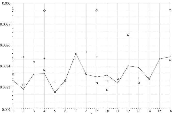
Fig. 1. The variance of the classical estimator 2ˆ(h)as a function ofhandd :d =1 (diamond), 2 (cross), 3 (square), 4 (line);N=212,=IN.
Note thatcov(qh∗
1, q ∗
h2) = 0 whenh1 = h2 andh1, h2 ∈/ H, and that the elements of
the matrix definingvdn(s1, s2, t1, t2)are positive. Thus, if thec(h)in (32) are positive and
non-decreasing in|H|, an increase in|H|must increasecov(qh∗ 1, q
∗
h2). Extensions to
higher-order cumulants are obvious, but, as in the case=IN, will entail a larger computational
burden. Finally, we note that the approach used here can also be extended to the case where the precision matrix−1, rather thanitself, is a linear combination of theAh.
3.3. Properties of the classical variogram estimator
The above results forqh provide the tools for studying the properties of the classical
variogram estimator for a second-order stationary and isotropic process under virtually any specification for thec(h). We do not intend to study the detailed properties of the variogram estimator here, but will show that the above results can be used to study the properties of 2ˆ(h) under a variety of specifications for the variogram 2(h) (for the intrinsically stationary, but non-isotropic case, see[5]).
We first consider the variance of 2ˆ(h) = qh/Nh as a function ofh andd, assuming
= IN. In Fig. 1 we plotvar(2ˆ(h)) = var(qh)/Nh2, computed using Eqs. (25) and
(28), ford = 1,2,3,4, andh = 1, . . . ,16, with Nheld fixed atN = 212, so that, for
d=1,2,3,4 we haven=212,26,24,23respectively.
Fig.1shows that: (a) for each fixed dimensiond >1, the variance is quite volatile as
r 0
0.0005 0.001 0.0015 0.002 0.0025
1 2 3 4 5 6 7 8 9 10 1 2 3 4 5 6 7 8 9 10
r 0
0.001 0.002 0.003 0.004 0.005
[image:16.468.64.414.81.201.2](a) (b)
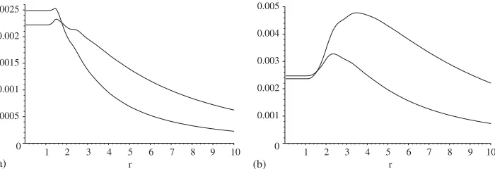
Fig. 2. The variance of the classical estimator 2ˆ(h)when the variogram is spherical. In (a)h=2, in (b)h=4 . The variance is plotted for many values of the rangerfrom 0 to 10,N=212,d=2 (thin line),d=3 (thick line).
h =9). Thus, in contrast to Fig. 4 in GGS (where the variance could only be computed for “non-diagonal” directions), our results show that when “diagonal” directions are taken into account—as it is natural to do under the assumption of isotropy—var(2ˆ(h))is no longer monotonic either indor inh. The volatility and non-monotonicity of the variances is attributable to variation inNh,mh, and the structure ofhashvaries. The explanation is
purely number theoretic: the number of decompositions of a particularhas a sum of squares is not related in any simple way to the valuesnandd.
The variance of the classical variogram estimator whenis of the form (32) can be computed using (37) withh1 = h2. Using this formula, one can study the behavior of
var(2ˆ(h))under various specifications for the true variogram 2(h), i.e., of thec(h)in (32). In Fig.2we plot the variances for the case of a spherical variogram with sill 1, nugget 0 and ranger, so that thec(h)in (32) are given by
c(h)=c(h, r)=
1−(3√h/r+(√h/r)3)/2 if 0hr2,
0 ifh > r2. (40)
The value ofNis kept fixed, as above, atN =212. We plot the variances ford =2 and
d =3 as a function of the ranger(the variogram is not valid ford >3). In Fig.2(a) we display the results forh=2 (note that this is a diagonal direction in the sense of GGS—for anyd), and in Fig.2(b) forh=4. The corresponding figure forh=1 is equivalent to Fig.
7 in GGS, which was produced by simulation forN =28(note that GGS appear to have
omitted a factor 2).
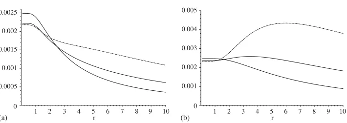
In Fig.3we repeat this exercise for the case of an exponential variogram with sill 1, nugget 0 and (practical) ranger, so that thec(h)in (32) are given by
c(h)=c(h, r)=exp{−3√h/r}, h0. (41)
G. Hillier, F. Martellosio / Journal of Multivariate Analysis 97 (2006) 1 – 18
1 2 3 4 5 6 7 8 9 10 0 1 2 3 4 5 6 7 8 9 10
r 0
0.0005 0.001 0.0015 0.002 0.0025
r 0.001
0.002 0.003 0.004 0.005
[image:17.468.56.411.74.200.2](a) (b)
Fig. 3. The variance of the classical estimator 2ˆ(h)when the variogram is exponential. In (a)h=2, in (b)h=4. The variance is plotted for many values of the (practical) rangerfrom 0 to 10, N=212,d=2 (thin line),d=3 (thick line),d=4 (dashed line).
those forh =4, in both cases ford =2,3, and 4 (the exponential variogram is valid for alld).
With a fixed number,N, ofi.i.d. observations, we expect the variance to decrease, at least for smallh(hNd1)asdincreases, because the number of pairs of points available to estimate 2(h)(for fixedh)cannot decrease asdincreases, and usually increases. But, as dependence in the data increases, orhincreases, one anticipates that this effect might be overturned. Both Figs. 2 and 3 show that these expectations are correct: the variances are not monotonic inr, sometimes increasing withrinitially, then decreasing. And the non-monotonicity is more pronounced for largerh, and for the case of a spherical variogram. Note that the lack of smoothness for low values ofrevident in Fig.2arises because the spherical variogram itself is not smooth. For sufficiently large values ofr—the values most likely to be used in applications—the variance for fixedhis increasing indfor both variograms—as suggested by GGS.
Of course, the usefulness of Lemma7is in providing a means to computevar(2ˆ(h))(and covariances) exactly in applications. For the exponential this is not a trivial computation, because as we note above,c(h) = 0 for all feasible values ofh, so that [SH(t )]in (33)
contains all feasible values. In practice, however, perfectly satisfactory accuracy can be achieved by truncating thec(h, r)at some point.
4. Concluding remarks
Fortunately, to study the properties of the associated quadratic forms the eigenvalues themselves are not needed: the generating functions for the matrices themselves induce generating functions for their cumulants. We provide detailed results on the means, variances and covariances of these statistics. As an important application of these results, we give simple formulae for the normalizing constant needed to produce an unbiased estimator of the variogram, and, assuming second-order stationarity, the covariance matrix needed to implement generalized least squares procedure for variogram estimation (see[6, Chapter 6]). Finally, we briefly study some properties of the classical variogram estimator for the cases of some popular choices of the actual variogram.
For the purposes of hypothesis testing the normalized statisticsq¯h∗=z′Ahz/z′zandq¯h=
z′Lhz/z′zare of greater interest. But since exact distribution theory for such statistics is
difficult, various techniques for approximating the distributions based on just the low-order cumulants have been developed (see, for instance,[1,8,12]). Although we do not implement them here, the results in Section 3 make such techniques quite straightforward. It is easily seen that, under the assumption that z∼N (0,2IN)—usually the null hypothesis—the
ratiosq¯h∗andq¯hare independent of their denominator, so that the moments of the ratios are
ratios of the moments. Hence the cumulant results forqh∗andqhgiven in Section 3 can also
be used to study or approximate the properties ofq¯h∗andq¯hunder this assumption.
It is, of course, both analytically and computationally convenient if the eigenvalues, or good approximations to them, ofLhandAhare known. One possible device for developing
approximations in the cased = 1 is to replace theFr by their circular counterparts (see
[2, Chapter 6.5]), and our results allow that approach to be adapted to higher dimensional cases straightforwardly. We will report our work on that subject elsewhere.
Acknowledgment
We thank two anonymous referees for helpful comments on an earlier version of the paper. FM acknowledges support from ESRC grant No. R42200134323.
References
[1]M.M. Ali, Durbin–Watson generalized Durbin–Watson tests for autocorrelations and randomness, J. Bus. Econom. Statist. 5 (1987) 195–203.
[2]T.W. Anderson, The Statistical Analysis of Time Series, Wiley, New York, 1971.
[3]M.J. Beeson, Triangles with vertices on lattice points, Amer. Math. Mon. 99 (1992) 243–252.
[4]J. Besag, Spatial interaction and the statistical analysis of lattice systems, J. Roy. Statist. Soc. Ser. B 36 (1974) 192–236.
[5]N. Cressie, Fitting varogram models by weighted least squares, Math. Geol. 17 (1985) 563–586.
[6]N. Cressie, Statistics for Spatial Data, Wiley, New York, 1993.
[7]D.M. Cvetkovi´c, M. Doob, H. Sachs, Spectra of Graphs, Academic Press, New York, 1980.
[8]J. Durbin, G.S. Watson, Testing for serial correlation in least squares regression II, Biometrika 38 (1951) 159–178.
[9]M.G. Genton, Variogram fitting by generalized least squares using an explicit formula for the covariance structure, Math. Geol. 30 (1998) 323–345.
G. Hillier, F. Martellosio / Journal of Multivariate Analysis 97 (2006) 1 – 18
[11]G.H. Hardy, E.M. Wright, An Introduction to the Theory of Numbers, fifth ed., Oxford University Press, Oxford, 1979.
[12]R.C. Henshaw, Testing single-equation least squares regression models for autocorrelated disturbances, Econometrica 34 (1996) 646–660.
[13]G.H. Hillier, The density of a quadratic form in a vector uniformly distributed on then-sphere, Econometric Theory 17 (2001) 1–28.
[14]A.T. James, Distributions of matrix variates and latent roots derived from normal samples, Ann. Math. Statist. 35 (1964) 475–501.
[15]M.G. Kendall, A. Stuart, The Advanced Theory of Statistics, vol. 1, Distribution Theory, Griffin and Co., London, 1969.
[16]M. Marcus, H. Minc, A Survey of Matrix Theory and Matrix Inequalities, Dover, New York, 1969.
[17]B. Mohar, Some applications of Laplace eigenvalues of graphs, in: G. Hahn, G. Sabidussi (Eds.), Graph Symmetry: Algebraic Methods and Applications, vol. 497 of NATO ASI Series C, Kluwer, Dordrecht, 1997, pp. 227–275.
[18]P.A.P. Moran, Notes on continuous stochastic phenomena, Biometrika 37 (1950) 17–23.
[19]J. von Neumann, R.H. Kent, H.R. Bellinson, B.I. Hart, The mean square successive differences, Ann. Math. Statist. 12 (1941) 153–162.