PERFORMANCE MEASUREMENT AND EVALUATION

Munich Personal RePEc Archive

PERFORMANCE MEASUREMENT

AND EVALUATION

Plantinga, Auke

University of Groningen

26 September 2007

Online at

https://mpra.ub.uni-muenchen.de/5048/

C

HAPTER

10.

P

ERFORMANCE MEASUREMENT AND EVALUATION

Auke Plantinga

Faculty of Business and Economics Department of Finance

University of Groningen The Netherlands

10.1 Introduction

This chapter discusses methods and techniques for measuring and evaluating performance for the purpose of controlling the investment process. However, many of the methods discussed in this chapter are also used in communicating investment performance between the investment management company and it’s (potential) customers. Therefore, performance measurements also play an important role in the competition between investments management companies. Substantial evidence from the net sales of mutual funds shows that investors buy mutual funds with good past performance records although they fail to sell funds with bad past performance2.

This chapter provides an overview of commonly used methods for measuring and evaluating the performance of investment management processes. In section 10.2 we discuss methods of calculating the returns of investment portfolios. We focus on the precision of such measures and the practical considerations in choosing a measure. In section 10.3 we discuss methods for evaluating performance, which are base on standard measures of risk such as standard deviation and Beta. In section 10.4 we present several alternative performance measures, which are based on measures of downside risk.

If the performance of a portfolio deviates from the benchmark, it is desirable to figure out what the causes of this deviation are. Performance attribution is the process of allocating the deviations from the benchmark performance to specific causes. In section 10.5 and 10.6, we discus performance attribution methods, which aim to link the outcome of the evaluation to specific parts of the investment management process. Section 10.5 deals with methods that use information on the portfolio composition in the analysis. Section 10.6 deals with methods that rely solely on the time series of returns of the portfolio. Finally, in section 10.7, we relate the performance of a portfolio to well-defined investment objectives that are related to the liabilities. These liability-driven attribution models are based on customized benchmarks.

1

© 2007, Auke Plantinga. This is a chapter of the reader ‘Investment Management: Theory and Practice’, edited by Robert van der Meer and Auke Plantinga

2

10.2 Measuring returns

10.2.1 Introduction

The total rate of returns of a portfolio is the relative change in the value of the portfolio including cash returns such as dividends and coupon payments. Total rate of return includes both realized and unrealized capital gains. The total return of a portfolio is defined as:

0 0 1 P C P P

R= − − , (10.1)

where P0 and P1 represent the market value of the portfolio at the start and end of the evaluation

period and C represents the net cash inflow (funding payments minus withdrawals) in the portfolio. In order to calculate the return of a portfolio, it is important to have a clear definition of the portfolio with respect to the inclusion or exclusion of cash. Some investors prefer to calculate the return of the portfolio inclusive of the cash position associated with the management of the portfolio.

Consider the following example of a portfolio that includes a cash position of 1000 at the beginning. Suppose that this portfolio is invested in 100 shares of Unilever stocks with a market price of 100 at the beginning of the period and 110 at the end. In addition, suppose that Unilever paid a cash dividend at the end of the period of 2 per share and the investor added another 500 to the portfolio. Therefore, the market value at the beginning is 11,000 and the market value at the end is 12,700. The total return on this portfolio is now equal to (12,700 – 11,000 – 500)/11,000 = 10.91%.

Alternatively, the return of the portfolio exclusive of the cash position is based on a beginning value of 10,000 and an ending value of 11,000 and a cash outflow of 200. This results in a return of (11,000-10,000+200)/10,000 = 12%.

For reporting purposes, it is convenient to summarize returns realized in subsequent periods. Returns are usually expressed as the annualized average return, using either arithmetic or a geometric return. An important issue it the way to handle intermediate cash flows to the portfolio, using either a time weighted or a money weighted return measure.

10.2.2 Arithmetic and geometric return

The difference between geometric and arithmetic return is important in measuring the performance of investment portfolios. Geometric return is defined as:

(

1

)

1

1

1

1 1 1 2 2 1 1 1 1 1

-P

P

-P

P

. . . .

P

P

.

P

P

-

R

+

MGR

=

=

=

_∏

the portfolio. For this reason, the geometric return is a suitable measure for an investor who wants to maximize his wealth at time T.

The (unweighted) arithmetic mean return is defined as:

R T

RGR = t

T

t=1

1

(10.3)

The arithmetic mean is a 1st order approximation based on a Taylor series expansion. A 2nd order approximation is:

- Rt T

t= T

MGR 2

2 1

1 1

≈ , (10.4)

where is the standard deviation of returns in individual sub periods.

Equation 10.4 implies that the geometric average is always smaller than the arithmetic average. Assuming that it is safe to ignore higher order terms from the Taylor series expansion, the difference between the arithmetic average return and the geometric average return is determined by the standard deviation. Consequently, an investor selecting risky alternatives based on arithmetic averages will choose the alternative with the highest standard deviation if both alternatives have the same terminal value.

The arithmetic average can be seen as an upward biased approximation of the geometric average. The following example is a clear illustration of this. Suppose that a stock returns +50% in year 1 and – 50% in year 2. The arithmetic average return over both periods is equal to 0%. However, this is a rather optimistic representation of the facts. Starting with an investment of € 1000, the investment grows to € 1500 at the end of period 1 and ends with only € 750 at the end of period 2. Effectively, the investor lost money, a fact that will be reflected in the geometric average mean return of –13.4%.

Although the geometric average mean appears to be the superior measure, it is also associated with some deficiencies. For example, section 10.4 discusses the problems with the use of geometric average return in attribution models. Another problem is that the normality assumption no longer holds for the distribution of geometric average. A solution for both problems is the use of continuously compounded return, which we denote with the lowercase symbol r:

P P r =

0 1

ln (10.5)

The average continuously compounded return over several sub periods is equal to:

r T =

CGR t

T t= ,T

1 1

1

(10.6)

where Rt is the return over period t calculated according to equation 10.5. The value of an invested of

e =

VT T CGR1,T (10.7)

Similar to the geometric average return, the average continuously compounded return is determined by the terminal value of the investment.

10.2.3 Time weighted and money weighted return

The difference between time weighted return and money weighted return is determined by the way both measures handle intermediate cash flows. A time weighted return measure accounts for the precise amount and timing of the intermediate cash flows, whereas the money weighted return measure is based on assumptions regarding amount and timing. Although time weighted return usually yields the most accurate return estimates, practical considerations may be in favor of a money weighted return measure.

Time weighted return

Time weighted return requires the evaluator to determine the market value of the portfolio each time a cash flow occurs. Next, the return on each time frame between two consecutive cash flows can be calculated and finally the evaluator can calculate the geometric average return over the different time frames.

Suppose that a cash flow occurs at time t, Pt is the market value of the portfolio an instant before time

t, and P_t*₋₁ is the market value just after the occurrence of the previous cash flow at t-1. Then, the return of the portfolio over the time frame starting at t -1 and ending at t is:

P P - P =

R *

t * t t t

1 1

− −

(10.8)

The annualized time weighted return over the period from t = 0 to T is equal to the geometric average of the returns of the individual time frames3.

(

) (

)

(

)

[

1

1

1

]

-

1

0

=

+

R

+

R

. . .

+

R

TWR

The following example illustrates the use of time-weighted return. Consider a portfolio with value € 100 at t = 0 that receives a funding cash flow of € 10 at t = 0.5. An instant before t = 0.5, the portfolio has a market value of € 105. At t = 1 the portfolio has a market value of € 120.75. Based on these numbers, we can calculate the time weighted return over the individual time frames as:

t = 0 .. 0.5 R0.5 = (105 - 100) / 100 = 5%

t = 0.5 .. 1 R1= (120.75 - [105 +10] ) / (105 + 10) = 5%

The annualized time weighted return over the period from t = 0 to t = 1 is:

t = 0 .. 1 TWR0,1 = (1.05) * (1.05) -1 = 10.25 %

3

Money weighted return

Money weighted return requires market values of the portfolio at the start and end of the evaluation period: there are no market values required at other moments. Alternatively, assumptions are made regarding the timing of the cash flows and the return path during the evaluation period. Money weighted return measures are convenient in a portfolio with many cash flows, since they avoid frequent valuations of the portfolio.

A well-known example of a money weighted return measure is the so-called Dietz algorithm4. The assumptions in this algorithm are that the cash flows occur in the middle of the evaluation period at t

= 0.5 and that the cash flow is reinvested at a return equal to the return of the portfolio, which is constant during the evaluation period. Given these assumptions, the terminal value of the portfolio is:

(

)

(

)

P =

PT 0 1 0, T 1 05 0,T (10.10)

This can be rewritten as:

C

P

C

P

P

MWR

T

5

.

0

0 0 ,

0

+

−

−

=

where P0 and PT are the market value of the portfolio at the begin and end of the evaluation period,

and C is the net cash flow during the evaluation period.

We can also calculate the money weighted return for the example introduced for explaining the time weighted return:

MWR0,1 = (120.75 - [100 + 10] )/(100 + 5) = 10.24 %

This example seems to suggest that the difference between time weighted return and money weighted return is very small. The small difference in this example is due to the fact that the assumptions made in the money weighted return are consistent with reality: cash flows indeed occur at the middle of the evaluation period, and the return in the first half of the period is exactly equal to the return in the second half. The remaining difference is due to fact that time weighted return is based on geometric average and the Dietz algorithm is based on arithmetic average.

The Banker’s Administrative Institute proposed a variant of the Dietz algorithm that uses compounded interest calculations. This so-called BAI algorithm calculates the return by solving

MWRb from the equation below:

(

)

(

)

0 1+MWR + C1+MWR

P =

Recalculation of our example using the BAI-algorithm yields exactly the same outcome as the time weighted return based on geometric average.

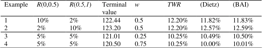
Table 10.1 provides some intuition on the impact of deviations from the assumptions for the outcomes of money weighted return measures. The table contains the outcomes of 4 examples of return calculations over an evaluation period consisting of two sub periods. The first column shows the example identifier, the second and third column provide the returns for the sub periods. The start value of the portfolio is 100 in all 4 examples, and size of the cash flow is 10. The fourth column gives the terminal market value of the portfolio, and the fifth column gives the time w of the cash flow. The last three columns present the outcomes for the time weighted return, the Dietz algorithm and the BAI algorithm.

Table 10.1: Examples with time and money weighted return calculations

Example R(0,0.5) R(0.5,1) Terminal value

w TWR (Dietz) (BAI)

1 10% 2% 122.44 0.5 12.20% 11.82% 11.83% 2 2% 10% 123.20 0.5 12.20% 12.57% 12.59% 3 5% 5% 121.01 0.25 10.25% 10.49% 10.50% 4 5% 5% 120.50 0.75 10.25% 10.00% 10.01%

4

See Dietz (1968). Another well-known example of a money weighted return measure is the internal rate of return, also known as the ‘yield to maturity’.

Examples 1 and 2 differ with respect to the order of the return path. In example 1, the return is high in the first sub period and low in the second sub period, whereas example 2 shows a reversed scenario. Comparing the outcomes of examples 1 and 2 shows that example 2 gives the highest terminal market value, which is due to the fact that the cash flow can be invested at a higher return. The time weighted return measure is the most appropriate measure for a portfolio manager who cannot control the timing (and size) of the cash flows. The table also shows that the Dietz measure underestimates the time weighted return if the return in the first sub period is higher than in the second sub period, and is an overestimation in the reverse case.

Examples 3 and 4 show the impact of deviations from the timing assumption The Dietz measure overestimates the return if the cash flow occurs earlier than assumed. If the cash flow occurs later than assumed, the Dietz measure is an underestimation of return. The modified Dietz measure allows for a more realistic assumption on the time of the cash flows, by choosing a value that relates to the actual average timing of the cash flows:

C

+

P

- C

P

-

P

=

R

τ

0 0

0 (10.13)

flow occurred at t = 0,25, the cash flow is 75% of the evaluation period present in the portfolio. The modified Dietz return is no equal to:

R0,1= (121.01 - 100 - 10)/(100+7.5) = 10.24%,

which is very close to the geometric average return.

10.3 Evaluating portfolio returns

Having calculated the total rate of return on a portfolio, the next step is to evaluate the return and identify whether or not the performance is satisfactory. Usually, this is accomplished by translating the investment objective into a benchmark portfolio. In the academic literature there has been a lot of emphasis on the difference between the risk of the portfolio and the benchmark. First, we discuss the methods developed by Jensen (1968), Treynor (1966), and Sharpe (1966), which focus on the differences in the levels of absolute risk of the portfolio and the benchmark. Next, we discuss the so-called relative measures of performance, which measure risk relative to the benchmark.

10.3.1 Jensen, Treynor and Sharpe performance measures

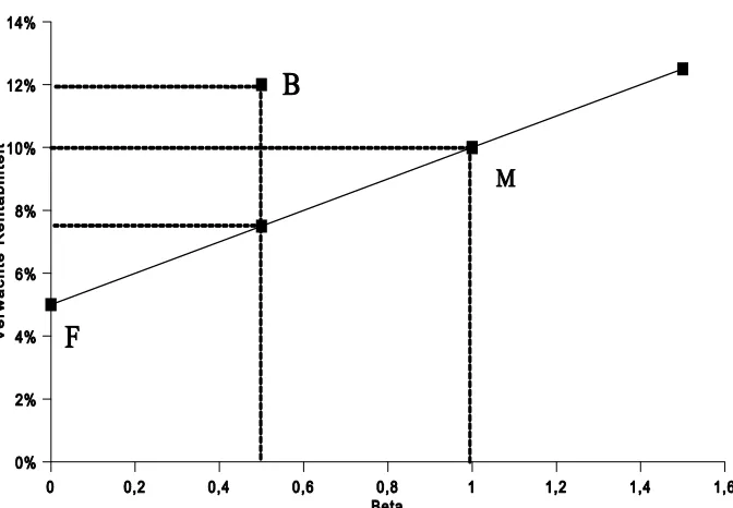
Figure 10.1: The capital market line

The Sharpe ratio

In the simple version of the CAPM, investors can lend or borrow risk free at the same interest rate. Therefore, an investor views all investment opportunities positioned on the CML as equally attractive, since risk free lending and borrowing enables him to replicate any position on the CML from another position on the CML. The only way to improve performance is to increase the angle of the CML.

The angle of the CML is also known as the Sharpe ratio which is defined as the ratio of expected return E(Rp) in excess of the risk free rate Rf and the standard deviation p of the portfolio:

[ ]

R

-

R

E

S =

p f p

(10.14)

With homogeneous expectations, it is not possible to find portfolios with a Sharpe ratio exceeding that of the market portfolio. However, active management implies heterogeneous expectations, which means that some portfolio managers may be able to construct portfolio with a Sharpe ratio that exceeds the market portfolio. For example, portfolio B in figure 10.1 has a Sharpe ratio equal to (12% - 5%) / 20% = 0.35 that exceeds the Sharpe ratio of the market portfolio (10% - 5%) / 20% = 0.25.

suitable investment. A more relevant criterion is to consider the Sharpe ratio of a portfolio of both European and South American stocks.

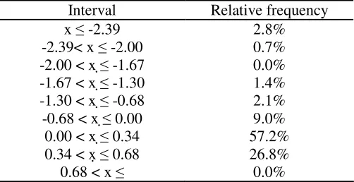
Despite this limitation, the Sharpe ratio is frequently used in performance reporting. In order to judge the Sharpe ratio of a particular portfolio, it is useful to have the distribution of Sharpe ratios of alternative portfolios. Table 10.2 presents a distribution of Sharpe ratios for 145 Dutch mutual funds calculated using monthly total returns over the period 1994-1998. The risk free rate is equal to the average money market return in this period. Most mutual funds have a Sharpe ratio between 0 and 0.34 and there are no funds with a Sharpe ratio over 0.68.

Table 10.2: Frequency distribution of Sharpe ratios of Dutch mutual funds over 1994-1998.

Interval Relative frequency

x -2.39 2.8%

-2.39< x -2.00 0.7% -2.00 < x -1.67 0.0% -1.67 < x -1.30 1.4% -1.30 < x -0.68 2.1% -0.68 < x 0.00 9.0% 0.00 < x 0.34 57.2% 0.34 < x 0.68 26.8% 0.68 < x 0.0%

Alternatively, the Sharpe ratio can be interpreted as a t-test for the hypothesis that the return on the portfolio is equal to the risk free rate. Since we do not observe Sharpe ratios over 1.96, we cannot reject this hypothesis for any of the mutual funds.

Jensen’s alpha

Figure 10.2: The security market line

With heterogeneous expectations, some investors may have an informational advantage resulting in return expectations that differ from the market’s expectations. Eventually, the informational advantage allows them to realize average returns above the security market line. For example, portfolio B has an expected return of 12% that exceeds the market expectation, which is 7.5% for a portfolio with a Beta of 0.5. The difference of 4.5% is Jensen’s alpha, which is defined as the difference between the realized return and the expected return given the beta of the portfolio.

Usually, Jensen’s alpha is measured with the following regression equation:

(

)

ε

+ = R -

Rp f p p m f , (10.15)

where Rm is the return on the market, p is the slope of the regression equation (the index of

systematic risk), and p is Jensen’s alpha. Using this equation we can calculate Jensen’s alpha for

portfolio B as

12% - 5% = p + 0,5 (10% - 5%) p = 4.5%

The Treynor ratio

The Treynor ratio is also derived from the SML. The Treynor ratio is the slope of the line connecting the actual portfolio with the risk free rate. If this slope exceeds that of the security market line, the portfolio has added value. The Treynor ratio is a measure of the return per unit systematic risk, and is defined as:

R - R T =

p f p

(10.16)

The outcome of the Treynor ratio is directly comparable with the equity premium, which is usually measured as the average of the difference between the market return and the risk free rate. If the Treynor ratio exceeds this equity premium, the portfolio manager has added value relative to a passive manager.

Problems with the use of JTS-measures

Normality and stationarity of the return distribution are important assumptions associated with Jensen’s alpha, the Treynor and the Sharpe ratio. In particular the assumption of normality may cause problems in case of portfolios managed with derivative instruments5. Bookstaber en Clarke (1985) used a simulation study to show that an investor without any forecasting skills can generate a Sharpe ratio in excess of the market’s Sharpe ratio by buying call options on the market portfolio. They consider three strategies, which are plotted in figure 10.3.

5

Figure 10.3: The capital market line with options

The first strategy is to invest 100% in the market portfolio. The second strategy is a portfolio C with 50% invested in the stock market portfolio and 50% in a long call option on the markt portfolio. The outcomes of the simulation study shows that this strategy results in a position above the capital market line, which implies that the Sharpe ratio of the portfolio exceeds that of the market portfolio. The third strategy is a portfolio P that invests 50% in the market portfolio and 50% in a long put option on the market portfolio. Figure 10.3 shows that this strategy actually plots below the capital market line.

10.3.2 Relative performance measurement

The Jensen, Treynor, and Sharpe measures of performance have been utilized extensively in both theory and practice. However, practitioners seem to favor relative performance measures. In particular, they focus on the performance relative to a benchmark without adjustments for systematic risk. Alternatively, they utilize the tracking error, which is the risk relative to the benchmark. They combine the relative return and relative risk measure into the so-called information ratio, which is the equivalent of the Sharpe ratio in relative risk and return space.

The information ratio

[ ]

[ ]

te m p E

E

(10.17)

where Rp is the return on the portfolio, Rm is the return on a representative market index and te is the

tracking error. Tracking error can be calculated using a time series of returns:

(

)

1 1

R -R

= _{p,t m,t}

T

t= T

te (10.18)

where Rp,t is the portfolio return in period t, Rm,t is the market index return in period t and T is the total

number of observed periods.

The information ratio can be interpreted as the t-test associated with the hypothesis that the returns on the portfolio do not significantly deviate from the market index. An information ratio larger than 1.96 implies that a portfolio manager has a 95% probability of beating the market index in any period.

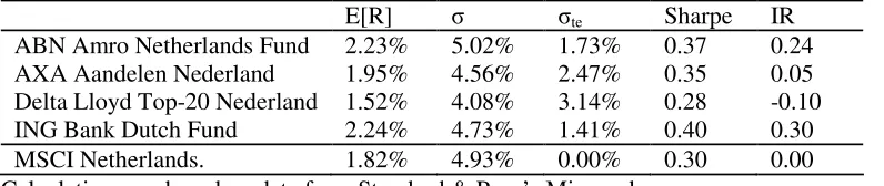
Table 10.3: Example of mutual fund evaluation using the Sharpe and information ratio

E[R] te Sharpe IR

ABN Amro Netherlands Fund 2.23% 5.02% 1.73% 0.37 0.24 AXA Aandelen Nederland 1.95% 4.56% 2.47% 0.35 0.05 Delta Lloyd Top-20 Nederland 1.52% 4.08% 3.14% 0.28 -0.10 ING Bank Dutch Fund 2.24% 4.73% 1.41% 0.40 0.30 MSCI Netherlands. 1.82% 4.93% 0.00% 0.30 0.00 Calculations are based on data from Standard & Poor’s Micropal

The third and fourth column presents respectively the standard deviation and the tracking error of the monthly returns. The numbers show that ABN Amro Netherlands Fund is the most risky fund in terms of total risk, although it’s tracking error ranks lower as compared to the other funds. There appears to be an association between the total level of risk and average return, since funds with a high total risk also have a high average return. It is also clear that the tracking error is not related to the level of total risk. Despite the fact that the risk measures result in different outcomes, the ranking of performance based on the Sharpe ratio and the information ratio is the same. However, the information ratio results in larger differences between the funds in terms of the score on the performance measure.

10.4 Alternative performance measures

This section discusses several risk-adjusted performance measures that allow for deviations from the traditional mean-variance framework. A major criticism of the mean-variance framework is its reliance on either the assumption of normally distributed returns or on the assumption of quadratic utility.

Several alternative performance measures are based on the concept of downside deviation. Downside deviation is a risk measure that deviates from standard deviation in two ways. First, it defines risk relative to an exogenous reference point. This reference point, which is also called the minimal acceptable rate of return, is used to distinguish ‘risk’ from ‘volatility’. According to Sortino and Van der Meer (1991), realizations above the reference point imply that goals are accomplished and, therefore, are considered ‘good volatility’. Realizations below the reference point imply failure to accomplish the goals and should be considered ‘bad volatility’ or risk. Second, downside risk only accounts for deviations below the reference point, and ignores deviations above the reference point. Downside deviation is defined as:

(

R

-

R

)

R

<

R

=

T t=

T

∀

2

1 1

δ

where is downside deviation and Rmar is the minimal acceptable rate of return.

[ ]

Sort= − . (10.20)

Another measure based donwside risk is the Fouse index, which is described in Sortino and Price (1994):

2

]

[R B

δ

E

Fouse = − , (10.21)

where B is a parameter representing the degree of risk aversion of the investor.

The Sortino ratio and the Fouse index rely on the use of expected return and downside risk. Expected return is used as a measure of the potential reward of an investment opportunity. An alternative for using the expected return is the so-called upside potential ratio, which is the probability weighted average of returns above the reference rate. The upside potential ratio was developed by Sortino, Van der Meer, and Plantinga (1999) and is defined as:

(

)

(

)

ι

ι

where T is the number of periods in the sample, Rt is the return of an investment in period t, +

=1 if

Rt>Rmar, +

= 0 if Rt Rmar,

-=1 if Rt Rmarand

-=0 if Rt>Rmar. An important advantage of using the

upside potential ratio rather than the Sortino ratio or the Fouse index is the consistency in the use of the reference rate for evaluating both profits and losses.

Finally, an important difference between downside risk and standard deviation is the use of an exogenous reference rate versus the mean return. The investor’s objective function motivates the choice of the reference rate. As a result, a part of the investor’s preference function is introduced into the risk calculation. Therefore, the resulting calculation is only valid for individuals sharing the same reference rate. Investors with different minimal acceptable rates of return will have different rankings.

10.5 Performance attribution

10.5.1 Introduction

that analyze both the portfolio composition and returns in identifying causes of deviations from the benchmark.

Most methods used in practice are derived from the framework used by Brinson and Fachler (1985). Many institutional investors use this method. The Brinson and Fachler framework is based on a top-down investment management process. Although the original version of this framework is only useful to support a very general analysis, it can be extended quite easily to support more realistic assumptions regarding the special properties of specific asset classes such as fixed income instruments and currency exposure.

In section 10.4.2 we discuss the Brinson & Fachler framework. In the next sections, we discuss the extensions to the simple framework. In section 10.4.3 we discuss how to analyze fixed income securities using the model of Fong, Pearson and Vasicek (1983) and in section 10.4.4 we deal with currency exposure using the method of Singer and Karnosky (1995).

10.5.2 The attribution model of Brinson and Fachler

The framework of Brinson and Fachler (1985) is based on well-known techniques from management accounting aimed at analyzing the differences between budgets and realizations. The framework corresponds to a top-down approach in the investment management process, starting from a general investment plan that describes planned portfolio weights for asset classes and assigns benchmarks to asset classes. The top level of management authorizes this general investment plan. The plan provides room for the lower levels in the organization to deviate from the plan in order to capture changing conditions in financial markets. Many professional investors have monthly or weekly meetings of portfolio managers and researchers to decide on tactical issues regarding deviation from the asset allocation. This decision is called the tactical asset allocation decision. Portfolio managers within asset classes also have different levels of discretion to deviate from their benchmarks. Actual deviations from the benchmark with an asset class are called stock selection decisions.

The analysis is based on four different portfolios: I. The benchmark portfolio; II. The stock-selected portfolio; III. The timing portfolio; IV. The actual portfolio.

Portfolio I is the overall benchmark portfolio, which is derived directly from the general investment plan. Portfolio I defines the desired asset allocation also known as the strategic asset allocation and the benchmarks for individual asset classes. Portfolios II and III are the outcomes of a ‘what if’ analysis that aim to measure the impact of decisions in isolation from the other decisions.

R

w

R(I) =

i

, (10.23)

where wi p

is the strategic weight of asset class i and Ri p

is the return of the benchmark for asset class i.

Portfolio II measures the return of implementing the stock selection decision, whilst ignoring the tactical asset allocation decision. Let the actual return of an investor in asset class i be Ri

a

, then the return on portfolio II is:

R

w

R(II) =

i

(10.24)

Portfolio III measures the return of implementing the tactical asset allocation decision without the stock selection decision. The asset class weights for this portfolio are equal to the actual weights wi

a

, and the securities within an asset class are exactly equal to the benchmark for the asset class. The return on this portfolio is:

R

w

R(III) =

i

. (10.25)

Portfolio IV is the actual portfolio subject of the analysis. The return on the actual portfolio is:

R

w

R(IV) =

i

(10.26)

The difference between the return of portfolio I and portfolio III is the so-called ‘timing effect’, and represents the additional return due to the tactical asset allocation. The return difference between portfolio I and portfolio II is the so-called ‘selection effect’ and shows the additional return due to stock selection.

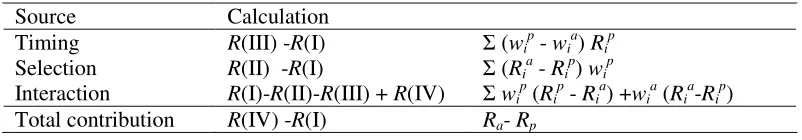
Since the timing effect and selection effect are calculated independently, we also need to capture the joint impact of both decisions, which is called the ‘interaction effect’. This effect is calculated as the sum of the return of portfolio I and IVminus the sum of the return of portfolio II and III. Since the interaction effect cannot be attributed to a single person or department, some practitioners allocate this effect in equal parts to both the timing and selection effect. The effects and their calculations are summarized in table 10.4.

Table 10.4: Components of the attribution model

Source Calculation

Timing R(III) -R(I) (wi p

- wi a

) Ri p

Selection R(II) -R(I) (Ri a

- Ri p

) wi p

Interaction R(I)-R(II)-R(III) + R(IV) wi p

(Ri p

- Ri a

) +wi a

(Ri a

-Ri p

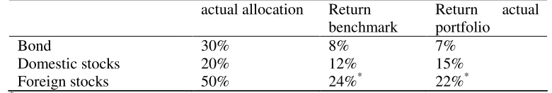
Suppose for example that an investor utilizes a strategic asset allocation of 50% bonds, 20% domestic stocks and 30% foreign stocks. Furthermore, assume that the actual allocation, the actual returns, and the benchmark returns are presented in table 10.5.

Table 10.5: Actual portfolio weights, benchmark returns and benchmark portfolio weights actual allocation Return

benchmark

Return actual portfolio

Bond 30% 8% 7%

Domestic stocks 20% 12% 15%

Foreign stocks 50% 24%* 22%*

*

Returns are measured in terms of the reporting currency.

The outcomes of the calculations for this example are given in table 10.6.

Table 10.6: Outcomes of the attribution model

Portfolio Return

I 13.6% Timing 3.2%

II 13.1% Selection -0.5%

III 16.8% Interaction -0.2%

IV 16.1% Total contribution 2.5%

This analysis shows that the investor in this example outperformed the overall benchmark by 2.5%, which is mainly due to considerable timing skills and not to selection skills.

Multi-period attribution

It is often desirable to summarize the performance attribution report over multiple periods. For example, many institutional investors generate quarterly attribution reports that they like to summarize on an annual basis. Since returns over multiple periods are usually calculated using a geometric average, problems may arise in summarizing the performance attribution. Table 10.7 provides an illustration of these problems.

Table 10.7: Multi-periodattribution

Period 1st half

of year

2nd half of year

overall

I 20.00% 10.00% 32.00%

II 17.00% 12.00% 31.04%

III 24.40% 12.00% 39.33%

IV 21.00% 14.25% 38.24%

Timing 4.40% 2.00% (a)

Table 10.7 presents performance attribution data on two periods. Performance presentation standards6 suggest that the return has to be summarized using a time weighted return measure, which involves the geometric average. In the fourth column of table 10.7 we present the geometric average return for the four portfolios from the attribution models.

The challenge to be faced is how to calculate the summarized outcomes (a), (b), (c), and (d) for the attribution components. An obvious solution is to calculate (a) as the difference betweenportfolio III and I over two periods: 39.33% - 32.00% = 7.33%. Unfortunately, it is not possible to link this number to the values for the timing component for each individual period: summing the individual answers results in a total of 6.4% and a geometric average on an annual basis results in 6.48%. Similar results can be found for the other components of the attribution model.

A solution to this problem is to calculate the return for the four portfolios based on continuously compounded average return, which is a time weighted return measure. In section 10.2.2 we found that the continuously compounded average return over multiple periods is an arithmetic average of the continuously compounded returns over the sub periods.

10.5.3 Portfolios with currency exposure

In this section we discuss the proposal by Singer en Karnosky (1995) to extend the model of Brinson and Fachler in order to deal with currency exposures. A distinct feature of the model is that local returns are analyzed in terms of risk premia. Singer and Karnosky argue that international interest parity conditions imply that currency returns depend on interest rate differences between countries. In particular, the pricing of currency forward contracts is determined to a large extent by interest rate differences. For this reason, they consider the effects of interest rate differences jointly with currency returns.

The return of an internationally diversified portfolio in terms of a base currency equals:

(

)

w =

Rbc i l,i bc,i , (10.27)

6

Time weighted return measures are required in order to be consistent with performance presentation standards such as GIPS.

where wi is the weight of country i as a fraction of the total portfolio value measured in terms of base

currency, Rl,i is the local currency return of an investment in country i and bc,i the relative value

change of the local currency i against the base currency.

Using currency forward contracts to hedge the currency risk completely, results in the following return in terms of base currency:

(

_R

+

f

)

w

=

HR

In hindsight, hedging provides the highest return if the realized currency return is lower than the return on the forward contract:

>

f

According to international interest parity, the return of the forward contract is equal to the difference in interest rates between the foreign country and the base currency:

c

-c

=

f

where cbc is the interest rate for the base currency and ci is the interest rate for the foreign currency i.

Therefore, equation 10.26 can be written as:

+ c > c

> c - c

bc,i i

bc

bc,i i

bc

(10.31)

These equations show that the interest rate differences and the currency returns are related. The return of a hedged foreign investment in terms of the base currency can be rewritten as:

HRbc,i = Rl,i + fbc, i = (ri – ci) + cbc (10.32)

The return of a non-hedged foreign investment in terms of the base currency is

Rbc,i = Rl,i + bc,i = (ri – ci) + (ci + bc,i) (10.33)

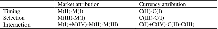
In other words, the return of any foreign investment in terms of the base currency can be written as a combination of (1) the local risk premium and (2) the relative change of an investment in the foreign currency. The second component is determined by the foreign interest rate and – if the foreign currency position is unhedged - the relative change in the value of the foreign currency. This decomposition is essential in the attribution model of Singer en Karnosky. Both components can be analyzed in terms of timing and selection attributes resulting in the market attribution for component (1) and the currency attribution for component (2). In table 10.8 we present the attribution framework for the market and the currency attribution.

Table 10.8: Attribution with currency exposure

Market attribution Currency attribution Timing M(II)-M(I) C(II)-C(I)

Selection M(III)-M(I) C(III)-C(I)

Interaction M(I)+M(IV)-M(II)-M(III) C(I)+C(IV)-C(II)-C(III)

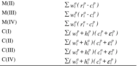
Following the method of Brinson and Fachler, each attribution requires 4 portfolios. In table 10.9 we show how to calculate the return on each portfolio.

Table 10.9: Return of the portfolios needed for calculating the attribution model

M(II) _{w (r -c}p₎ i p i a i

M(III) _{w (r -c}p₎ i a i p i

M(IV) _{w (r -c}p₎

i a i a i

C(I) _{(w +h )(c +} p₎

i p i p i p i

ε

C(II) _{(w +h )(c +} p₎ i p i a i a i

ε

C(III) _{(w +h )(c +} p₎ i a i p i p i

ε

C(IV) _{(w +h )(c +} p₎ i a i a i a i

ε

10.5.4 Fixed income securities

The nature of a portfolio of fixed income securities justifies a tailor-made evaluation method. For most fixed income instruments, the most important factor driving returns is interest rate risks. Unfortunately, the exposure to this factor is not constant since portfolio managers can change this exposure with a few transactions. Furthermore, the exposure to interest rate risk is declining with the passing of time. Therefore, we need a procedure specific for fixed income instruments for dealing with systematic risk. Fortunately, pricing of fixed income instruments is facilitated by the fact that prices can be approximated adequately with analytical price expressions. This allows us to deal with the interest rate risk exposure.

The price of a plain vanilla government bond is:

(

)

(

)

T t

t T

t=

+r

,T

H

+

,t

+r

C

P=

]

0

[

1

]

0

[

1

. (10.34)

where Ct is the coupon payment at t, HT is the face value at maturity T, and r[0,t] is the interest rate

for a zero coupon bond originating at t=0 and ending at t.

Fong, Pearson en Vasicek (1983) proposed a method for analyzing the returns of a portfolio of fixed income instruments. The following procedure is based on their model.

Table 10.10: Attribution model for fixed income instruments

Expected return

In table 10.10 we present the schedule for analyzing the returns of fixed income portfolios. The schedule is based on five additional benchmark portfolios that facilitate the decomposition of the return into external factors and skills of the portfolio manager. The external factors refer to the level and changes in the level of the interest rates. The skills of the portfolio manager reflect the effect of management on the portfolio return. For example, the effect of a rise in interest rates is an external factor since it is not a skill of the manager. However, the anticipation of the manager on this increase in interest rates by decreasing the portfolio duration is a skill.

Alternatively, it is possible to distinguish between the factors that drive the prices of fixed income instruments, such as interest rates, liquidity and credit risk. In the schedule, we limit our attention to interest rates and credit spread, although it is possible to extend the schedule. Consistent with the usual approach in performance attribution models, Fong, Pearson and Vasicek use several auxiliary portfolios to facilitate their analysis.

Portfolio II is used to measure the external interest rate effect, which cannot be attributed to specific actions of the portfolio manager. This effect can be decomposed into an expected part (measured by portfolio I) and an unexpected part (the difference between portfolio II and I). The difference between portfolio III and portfolio II is the return due to maturity management, which measures the added value of anticipating interest rate movements.

The difference between portfolio III and IV measures the impact of a portfolio manager’s choice for specific sectors in the bond market, such as the choice for bonds originated in the financial sector or specific industries. Finally, the difference between portfolio IV and V refers to the added value of bond picking.

The impact of interest rates on portfolio return

The level of the interest rates and changes in the level drives the impact of interest rates on the portfolio return. In addition, the portfolio manager can anticipate on changes in interest rates by increasing or decreasing the duration of his portfolio.

In order to separate the management effect from the external effect, it is necessary to choose a benchmark that corresponds with the investment objective. This implies that the benchmark has an adequate risk profile, by choosing appropriate levels of duration, convexity or other measures of interest rate risk. The external component is measured by calculating the present value of both the benchmark and the actual portfolio based on the term structure of risk free interest rates. This procedure eliminates the impact of other factors, such as credit risk and liquidity risk.

portfolio. The cash flows from both portfolios are discounted with the term structure of risk free interest rates.

Portfolio I measures the impact of the level of the interest rates. This portfolio is assumed to be invested at t = 0 in zero coupon bonds with maturity equal to the evaluation horizon. The return on this portfolio is equal to R(I)=r[0, t]. Portfolio I can also be seen as an investment in the money market.

The value of portfolio II is equal to the present value of the cash flows from the benchmark portfolio discounted with the term structure of risk free interest rates:

(

+ r

t,i

)

.

C

=

P

p,i T

i = t

t ₋

]

[

1

(II)

where Cp,i the cash flow for the benchmark portfolio at time i and r[t,i] the interest rate for a zero

coupon originated at time t that matures at time i.

The return of portfolio II measures the external effect of the interest environment on the benchmark return. The return of portfolio II is also affected by the investor’s choice for a benchmark with a particular duration. Consequently, the portfolio manager does not have control over this return. The external effect of the interest environment can be decomposed into an expected component R(I) and an unexpected component R(II) - R(I). The expected component is equal to the rate for a bond with a maturity equal to that of the investment horizon, the unexpected component is equal to the impact of a change in interest rate levels.

The value of portfolio III is equal to the present value of the cash flows from the actual portfolio discounted with the term structure of risk free interest rates:

(

)

a,i T

i = t t

t,i

+ r

C

(III) =

P

]

[

1

where Ca,idenotes the cash flow in the actual portfolio at time i.

The return of portfolio III measures the impact of the interest rate environment on the return of the actual portfolio, including its impact on the portfolio manager’s decision to choose a maturity structure different from that of the benchmark. Therefore, the difference between the return of portfolio III and portfolio II is entirely due to the difference in the timing of the cash flows. Consequently, the difference between portfolio III and II measures the impact of the decision of the portfolio manager to choose a duration different from the benchmark. This difference is labeled as the ‘effect of maturity management’ or the ‘duration effect’.

Example (1)

corresponding benchmark are presented in table 10.11. In addition, this table presents the term structure of risk free interest rates at t=0 and t=1.

Table 10.11: Cash flows and termstructure for evaluating portfolio ZZZ

Projected cash flows Term structure

Time Portfolio Benchmark t = 0 t = 1

1 1 000 5.00 % -

2 1 000 6.00 % 6.50 %

3 1 000 6.50 % 6.00 %

4 1 000 1 000 7.00 % 5.75 % 5 1 000 1 000 7.25 % 5.00%

Portfolio III Portfolio II

t=0 t=1 t=0 t=1 Present Value 1 468 1 668 4 138 4 497

Return 13.67 % 8.69 %

Based on this information, the present value of portfolio II and III can be calculated. The outcomes are given at the bottom rows of table 10.11. In this example, the effect of maturity management is

R(III) - R(II) = 13.67% - 8,69% = 4.99%. The external effect of the interest environment is 8.69%, which can be decomposed into an expected component of 5.00% and an unexpected component of 3.69%.

Credit risk

Credit risk is the second important factor in determining the return of a portfolio of fixed income instruments. Credit risk refers to the possibility that the debtor is not able to service the scheduled coupon and redemption payments on a bond. Credit risk is measured by rating agencies such as Fitch, Standard & Poor’s en Moody’s. Investors require a premium for credit risk that is increasing with the amount of risk. Therefore, a portfolio of corporate bonds is expected to yield a higher return than a portfolio of government bonds with similar maturities. In addition, a portfolio manager can add additional return by anticipating changes in the credit risk of individual corporations or entire sectors of the bond market. The anticipation of changes in the credit risk of individual corporations is called ‘bond picking’ and the anticipation of sectors is called ‘sector management’.

The contribution of sector sector management is calculated by valuing each individual bond at the begin and end date of the evaluation period based on the risk free discount rate and a premium for credit risk equal to that of the sector average. The return of the portfolio based on these valuations is the return on portfolio IV. The contribution of sector management is equal to the difference between the return on portfolio IV and III.

Example 1 (Continued)

Table 10.12: Cash flows and term structures for different credit risk classes

A B A B A B

1 6.00 % 7.00 % - -

2 7.00 % 8.00 % 8.50 % 8.50 %

3 7.50 % 8.50 % 8.00 % 8.00 %

4 300 700 8.00 % 9.00 % 7.75 % 7.75 %

5 600 400 8.25 % 9.25 % 7.00 % 7.00 %

Suppose that the cash flows of portfolio ZZZ can be decomposed in two credit risk categories according to table 10.12. At t = 0 the credit risk premium is 1% for A-rated bonds and 2% for B-rated bonds. At t=1, the credit risk premium for both categories is equal to 2%. For reasons of simplicity, we assume that the credit risk premium is unrelated to the maturity of the loan. Based on this information, we can construct a term structure for both credit classes by adding the credit risk premium to the term structure of risk free discount rates.

The value of portfolio IV – decomposed into different sectors - is calculated using the term structures presented in table 10.12. The outcomes of these calculations as well as the return on portfolio IV are presented in table 10.13.

Table 10.13: Value of portfolio IV decomposed into sectors

A B Total

Present value t=0 624 753 1 377 Present value t=1 698 865 1 563

Return R(IV) 13.45 %

The contribution of sector management is now equal to R(IV) - R(III) = -0.22 %. This contribution can be compared against the contribution of sector management in the benchmark portfolio.

Bond selection

Fong, Pearson, and Vasicek (1983) identify the remaining difference between the actual return (portfolio V) and portfolio IV as a measure of bond selection ability. The accuracy of this measure depends on the validity of the implicit assumptions underlying this method, such as the following assumptions:

the portfolio is invested in fixed income securities, without option features, such as call and put features.

the portfolio is invested in one currency.

the bond markets are very liquid and do not require liquidity premia.

between this portfolio and the actual portfolio represents the effect of ‘option-adjusted spreads’7. In general, the actual decision to refine the measurements depends on the magnitude of the deviations from the assumptions and needs to be weighted against the required resources to implement the refinements.

Table 10.14: Attribution of a fixed income portfolio.

Component Portfolio

Expected return 5.00 % I

Unexpected return 3.69 % II - I

External effect 8.69% II

Maturity management 4.99 % III - II Sector management - 0.23 % IV - III

Selection 1.94 % V - IV

Total management 6.70% V - II

Total 15.38% V

7

This chapter does not explicitly deal with the calculation of option-adjusted spreads. We refer the interested reader to for example, Hayre (1990) or Babbel and Zenios (1992).

10.6

Attribution of performance using time series of returns

10.6.1 Introduction

In the previous section, we used information on the portfolio weights in order to get a performance attribution. However, the portfolio composition is not always available for the performance analyst. In this section we discuss performance attribution methods based on the analysis of time series of returns.

10.6.2 Treynor and Mazuy

Based on this assumption, they propose to measure selection and timing ability, by fitting following curve on the time series of return of the portfolio and the market index:

(

)

(

)

2 1

0 p f p f

f

a R TM TM R R RM R R

R − = + − + − (10.37)

where TM0 is a measure of the portfolio manager's selection ability and TM2 is a measure of the fund's

timing ability. If the manager has selection ability, then TM0 > 0, and if the manager has timing

ability, then TM2> 0.

10.6.3 The parametric test of Henriksson and Merton

Henriksson and Merton (1981) developed two methods of performance evaluation based on the option-like payoff structure of a managed portfolio's return. One of these methods is called the parametric test, and can be used to measure selection and timing ability.

The parametric test of Henriksson and Merton (1981) is derived from a model of the value of forecasting abilities developed by Merton (1981). In this model, there is a perfect market timer who is able to predict whether or not the return on the stock market will exceed the risk free return. In effect, the market timer will invest in the risk free fund if a down-market is expected, and in the stock market if an up-market is expected. The return from this strategy corresponds to investing in a stock portfolio and put options or investing in a cash portfolio with call options. The perfect market timer is likely to be fictional, so the important issue is to assess to what degree market timers possess timing ability.

The parametric test of Henriksson and Merton (1981) allows for market forecasters that have less than perfect forecasting skills. This test is based on the following assumptions:

The portfolio manager makes forecasts of a specific type: the forecast is that either the return on the stock market exceeds the return on the risk free asset (an up-market), or the return on the risk free asset exceeds the return on the stock market (a down-market).

The probability of a correct down-market forecast is identified by p1 and the probability of a correct

up-market forecast is identified by p2. This means that the model allows for the possibility that the

reliability of the forecasts can be different in up- and down-market forecasts.

The portfolio manager reacts on this forecast by choosing a portfolio with 1 if a down-market is

predicted, and 2 if an up-market is predicted.

The return process of the underlying assets is consistent with CAPM8.

Merton shows that if p1+p2>1, then the portfolio manager has forecasting skills and p1+p2=2 means

that the portfolio manager has perfect forecasting skills.

The method is implemented using the following regression equation:

8

( )

(

)

(

(

)

)

R_a = ₎ + _{1 m} − _f + _{2 n} − _f + , (10.38)

where Rm(t) is the return on the market portfolio, Rf(t) is the return on the risk less asset, and (t) is a

residual term satisfying the usual conditions. The term max(Rm(t)-Rf(t),0) can be seen as the payoff of

a long put option.

With this regression equation, the evaluator is able to test whether or not the changes in are on average adequate, by testing H0: HM2 = 0. If HM2 is significantly positive, then the portfolio manager

exhibits superior timing skills. If HM0 is significantly positive, then the portfolio exhibits superior

selection skills.

Henriksson and Merton showed that the probability limits of the least squares estimates of HM1 and

HM2 can be written as:

[ ]

(

)

[ ]

[ ]

(

)(

)

2 1 2 2 2 2 1 1 lim 1 lim

β

β

ω

ω

β

β

ω

where = -E[ ]. These estimates of HM1 and HM2 are consistent with Merton's equilibrium value

of market forecasts. If the manager has forecasting skills ( p1+ p2>1) and the manager behaves

rationally ( 2> 1) then HM2>0.

10.7

Liability-driven performance attribution

10.7.1 Introduction

The design of a system of performance measurement and evaluation should be closely linked to the investment philosophy of the investor. The most obvious way of obtaining this link is through the choice of the benchmark portfolio. The objective of the investor is the main determinant of the benchmark choice. However, the investment philosophy not only affects the investment objective, but also the design of the investment process. The components of the performance attribution should be a reflection of the decisions in the investment process.

Babbel and Hogan (1992) showed that the strategy of excessive risk-taking is not necessarily beneficial to shareholders. In particular, if policyholders are not convinced that their interests will be protected, they are likely to demand higher returns for their policies in order to compensate for the higher risks. Higher liability returns reduces the benefits of shareholders. Eventually, this could lead to a situation where shareholders’ value is lower compared to the situation where the asset portfolio has low risk.

Babbel, Stricker and Vanderhoof (1999) proposed a model for evaluating and controlling the performance of insurance companies that focuses both on the objective of shareholder value maximization and liability preservation. Their model is based on an analysis of the difference between asset and liability returns, and starts from the construction of so-called liability benchmarks. A liability benchmark is based on a portfolio of actively traded securities, and the return of the benchmark mimics the return of the market value of the liabilities over time. Next, an overall asset benchmark is created based on a separate optimization algortihm. The resulting overall asset benchmark is a maximization of the total rate of return of the assets subject to the condition that asset returns should outperform the liability benchmark returns. An alternative way of constructing a benchmark can be found in Leibowitz, Kogelman, and Bader (1992), who construct a portfolio that maximizes the asset return subject to conditions on the surplus returns. By comparing the return of the actual asset portfolio with the return on the overall asset benchmark, the value added by the asset management process can be measured and attributed to different sources.

The model we propose is different from the model proposed by Babbel, Stricker, and Vanderhoof (1999), although it shares many similarities as well. The main similarity is the central role of the liability benchmarks. However, in contrast with the Babbel, Stricker and Vanderhoof model, we compare the realized asset returns directly with the returns of the liability benchmarks, instead of creating an additional overall asset benchmark. Our motivation for skipping the step of the additional overall asset benchmark is that the liability benchmark is the most efficient portfolio from the perspective of the policyowner. By using the overall asset benchmark instead of the liability benchmark for evaluating the asset portfolio, a potential agency problem is created which could result in excessive risk taking at the expense of the policyowner. In other words, our model places more weight on the interests of the policyowner9.

Another difference is that our model is expressed in terms of surplus returns, which means that the degree of financial leverage plays an important role in the analysis. Sharpe and Tint (1992) showed that in the context of a Markowitz portfolio optimization, the degree of financial leverage has an impact on the optimal asset allocation for an investor with liabilities. This conclusion is also shared by Leibowitz, Kogelman and Bader (1994), who use a related measure, the funding ratio return, in the context of pension fund asset allocation. From a more practical point of view, financial leverage should play a role in a performance attribution model as it emphasizes the fact that leverage increases

9

the effect of any decision within the insurance company on shareholder value. Our model also makes an explicit distinction between the part of the asset portfolio that is used to cover the liability claims and the part of the asset portfolio that can be used to pay dividends to the shareholder. This distinction is caused by the extra emphasis on the objective of the policyholders. As a consequence the investment manager in our model can decide to deviate from the benchmark with respect to the allocation of funds over these two portfolios.

10.7.2 Liability-driven performance attribution

In this section, we develop a return attribution model that accounts for both the objective of liability preservation and the objective of surplus maximization. Taking a shareholder perspective, Elton and Gruber (1992) showed that part of the optimal asset portfolio of an investor with liabilities consists of cash flow matching assets. The market value of the cash flow matching assets in the optimal portfolio will be equal to the market value of the liabilities. We define the asset portfolio with cash flow matching assets as the liability-driven asset portfolio. The liability-driven asset portfolio combined with the liabilities forms a riskless portfolio.

Elton and Gruber showed that the remaining part of the optimal asset portfolio, which we will define as the surplus-driven portfolio, consists of risky assets. Depending on the institutional investor’s risk aversion, he can choose to replace part of the risky assets in the surplus-driven portfolio with an investment in zero-coupon treasury bonds. Based on the distinction between liability-driven and surplus-driven assets, we develop the following performance evaluation model10. The variables included in this model are presented in the following balance sheet:

Surplus-driven assets As Surplus S Liability-driven assets Al Liabilities L

Total A Total S+L

The benchmark of the institutional investor in this model has L/S cash matched investments and S/S assets with limited liability. All assets and liabilities are valued at market value. The liability-driven investments are the assets that are intended for replicating the return and risk characteristics of the liabilities. This is an important assumption in the analysis: it should be possible to replicate the return distribution of the liabilities with some asset portfolio. Liabilities expressed in nominal terms, such as bank deposits and life insurance, can be replicated reasonably well with default-free fixed income securities.

10