Effect of Spark Timing on Combustion Process of SI Engines using MATLAB

(1)

Effect of Spark Timing on Combustion Process of SI

Engines using MATLAB

Amit Karkamkar

Final Year Student Mechanical Engineering

ABSTRACT

The spark timing plays a significant role in the combustion process and in deciding the engine parameters of SI engine. This paper aims at demonstrating the effect of advanced and retarded spark timing on the burn fraction variation versus crank angle, cumulative heat release rate versus the crank angle and the pressure variation as a function of crank angle with the help of MATLAB programs. For this purpose, a basic finite heat release model is used for the combustion process in SI engines. This model can also be extended to evaluate effect of spark timing on engine work and thermal efficiency. In each section of the paper, the codes used for analysis are provided for future research work. Salient results, such as peak pressure crank angles for different spark timings , are derived from analysis.

Keywords

Finite Heat release model, SI engine, Combustion, MATLAB

1. INTRODUCTION

Ignition timing is very important for improving performance of modern SI Engines [5]. In an ideal four stroke SI engine, compression and expansion take place during 180° of crank rotation and combustion takes place instantaneously at TDC. During combustion the volume remains constant and there is a sudden pressure rise [1]. However, in an actual spark ignition engine, combustion does not occur instantaneously. It is initiated by a spark produced before TDC at a definite time which affects the maximum pressure generated and the corresponding crank angle, indicated mean effective pressure, and consequentially the work done in cycle and so the thermal efficiency. Studies have been conducted to demonstrate some of these effects previously [8]. This paper essentially aims at generating MATLAB programs which will take input of spark timing and will give output of the required engine parameters so that salient conclusions can be drawn. Computer models of engine processes are important tools for analysis of engine performance [6].

2. MASTER PROGRAM

As mentioned earlier, In this paper MATLAB codes are provided for further research work, which can be applied to any SI engine. So a master program is first written which will be used to input the engine data for every individual code. This is the function where the spark timing will be entered along with other engine specific data.

code:

function enginedata

bore = input('Value of diameter of Engine Cylinder = ');

stroke = input('Value of piston stroke = '); rc = input('Designated compression ratio = '); Vs = (pi/4)*(bore^2)*stroke;

l = input('length of connecting rod = '); R = 2*l/stroke;

thetad = 4*pi/9;

burnfractionvariation(thetas) heatrelease(thetas)

end

The functions heatrelease, burnfractionvariation are defined and described in the coming sections along with the results from their execution.

Sample Input Window:

FIG. 1

3. FINITE HEAT RELEASE MODEL

Finite heat release model evaluates the effect of spark timing on heat release in combustion process and mathematically models, in differential form, the pressure variations with respect to the crank angle [1]. It is a differential form of a mathematical model of the power cycle in which the heat release is expressed as a function of the crank angle.

3.1 Burn Fraction Variation

A typical heat release curve consists of the initial ignition lag(flame development) followed by flame propagation and flame termination [6]. Heat addition rate is zero for most of the cycle. Weibe function [1,9] or 'S' curve describes the fraction of fuel that has been burned. This function is represented mathematically by

( )

1 exp

n s b

d

x



a

 





_

_

_



 





_

_















……….(1)

where,

x

_b

( )



= Burn fraction as a function of crank angle



= Crank angle



_s= Spark timing



_d= Duration of heat release n = Weibe form factor a = Weibe efficiency factor

(2)

s



the burn fraction will be zero and after (



_s+



_d) it will be one.

Code:

function burnfractionvariation(thetas) thetad = 4*pi/9;

theta = -pi:0.1:pi; bb = ones(1,63); i = 1 ;

while i < 64

if theta(:,i)< thetas xb = 0;

elseif theta(:,i) > thetas + thetad xb = 1;

else

xb = 1 - exp(-5*(theta(:,i)-thetas/thetad)^3);

end

bb(:,i) = xb; i = i + 1;

end

subplot(2,2,1), plot(theta,bb) xlabel('Crank Angle')

ylabel('Burn Fraction Xb') axis([-pi pi 0 1])

end

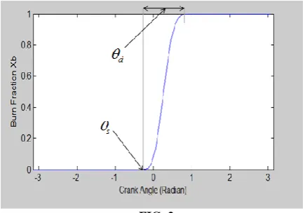
Output: (1) If the spark is initiated 20° before TDC the burn fraction variation is shown in FIG 2

FIG. 2

3.2 Heat Release Rate

In order to find the differential equation governing the heat release rate, eq.(1) is differentiated with respect to θ.

1

1 exp

.

n n

b s s

d d d

dx

a

an

d

 







_

_

_

 

_

_

_



 





_

_

 



_

_









 









 



1

(1

)

n s b

d d

an

x

 











 

_

_





The rate of heat release as a function of crank angle is

b in

dQ

dx

Q

d





d



1

(1

)

n

in s

b

d d

dQ

Q

an

x

d

 















_

_





………(2)

here,

Q

_in is the heat supplied by the fuel. When the combustion process is not happening this derivative is zero.

Thus, equation (2) gives the rate of heat release as a function of crank angle.

In this research work, the typical values of constants a and n are taken 5 and 3 respectively. However, they depend to some extent on engine load, speed and type of engine [1].

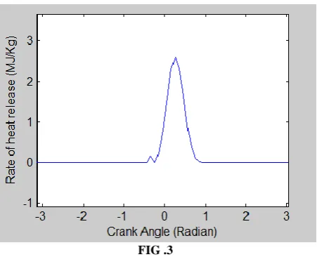
Following MATLAB code was written for analysis of heat release rate versus crank angle:

Code:

function heatrelease(thetas) thetad = 4*pi/9;

theta = -pi:0.1:pi; bb = ones(1,63); cc = ones(1,63); i = 1 ;

while i < 64

if theta(:,i)< thetas xb = 0;

elseif theta(:,i) > thetas + thetad xb = 1;

else

xb = 1 - exp(-5*(theta(:,i)-thetas/thetad)^3);

end

bb(:,i) = xb; i = i + 1;

end

i = 1;

while i < 64

if theta(:,i)< thetas hr = 0;

elseif theta(:,i) > thetas + thetad hr = 0;

else

hr = (5*3*1.8/thetad)*(1-bb(:,i))*(theta(:,i)-thetas/thetad)^2 ; end

cc(:,i) = hr; i = i + 1;

end

subplot(2,2,3),plot(theta,cc) xlabel('Crank Angle (Radian)')

ylabel('Rate of heat release (MJ/Kg)') axis('equal')

end

[image:2.595.55.273.353.505.2]

(3)

FIG .3

[image:3.595.56.282.69.252.2]

(2) If spark is initiated at crank angle 180° , then the heat release rate will be entirely zero as shown in FIG. 4

FIG. 4

3.3 Piston Volume Sweep

The geometry of the piston, the connecting rod and the crank [1] is shown in FIG. 5.

FIG. 5



= angle which connecting rod makes with centreline

θ = crank angle from TDC position a = crank radius ; l = connecting rod length From the FIG 5,

l sin





a

sin



The distance s is given by

s =

a

cos





l

2



a

2

sin

2



Thus, the piston displacement from TDC is x = l + a - s

=

l

 

a

cos





l

2



a

2

sin

2



Instantaneous cylinder volume,

c x

V



V



V

= 2

4

c

V





d x

2 2 1/2

[

1 cos( ) (

sin ( )) ]

(

1)

2

s s

V

R

r



 



 



…....(3)

Where, r = compression ratio and R =

l

a

s

V

= Displaced volume

c

V

= Clearance Volume

Now, differentiating above equation with respect to ϑ ;

2 2 1/2

sin( )[1 cos (

sin ( ))

]

2

s

dV

V

R

d











…(4)

[image:3.595.54.283.298.467.2]

The variation of the volume swept with respect to crank angle is graphically represented in FIG .6

FIG. 6

3.4 Pressure - crank angle relation

From the first law of thermodynamics applied for a closed system ;

Q

W

dU

   

But for reversible processes;

v

Q

pdV

mc dT

[image:3.595.316.564.469.666.2]

(4)

pV



mRT

pdV



vdP



mRdT

………(5)



mdT

pdV

Vdp

R





………....(6)

From eq .(4) and (5) ;

(

1)

R

pdV

Vdp

Q

pdV

R









 



_

_

 



1 



(

1)

pdV

Vdp









Differentiating with respect to



;

1 .

.

(

1)

(

1)

dQ

pdV

Vdp

d





















(

1)

dp

dQ

p dV

d

V

d

V d











……….(7)

Equation (2) for

dQ

d



and equation (4) for

dV

d



and equation

(3) for V are substituted in equation (7) ; the term

dp

d



is obtained as a function of crank angle



. This term is integrated numerically using fourth order Runge-Kutta method for pressure at different crank angles. In MATLAB this type of integration is carried out by the function ' ode 45'.

[3] First, a function is defined containing the equation (6). Then that function is called in the syntax as shown below for integration.

>> thetaspan=[-pi pi]; >> p0=10^5;

>> [theta,p] = ode45('pressure',thetaspan,p0); >> plot(theta,p)

The term p0 represents the initial condition. At the end of the suction stroke, the atmospheric pressure will ideally be equal to the pressure in cylinder. So accordingly value of p0 is

assigned in

N m

/

2. The function 'pressure' can be defined in various ways. Suppose pressure crank angle variation is to be found out for spark advance of 40° , following function was used in this analysis:

code:

function pdot = pressure(theta, p ) Vs = 7.8540e-004;

R = 3; rc = 10;

thetas= -4*pi/18;

pdot =(-(6*exp(-5*((theta-

thetas)/4*pi/9)^3)*((theta- thetas)/4*pi/9)^2)/((Vs/rc-1)+(Vs/2)*((R+1-cos(theta))-(R^2-sin(theta)^2)^0.5)) + (0.7*p*Vs*sin(theta)*(1+(cos(theta)*(R^2 - sin(theta)^2)^-0.5)))/((Vs/rc-1)+(Vs/2)*((R+1-cos(theta))-(R^2 - sin(theta)^2)^0.5)));

end

It is observed in the output of the above program that in this case for 40° spark advance ,the maximum pressure occurs

exactly at TDC. In similar way, for different spark timing analysis was done for pressure variation with respect to the crank angle. The crank angle at which peak pressure was generated in the p-



plot for each particular spark timing was noted down.

4. RESULTS FROM FINITE HEAT

RELEASE MODEL

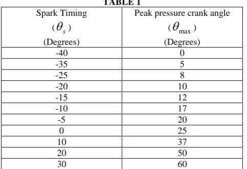
[image:4.595.309.551.233.398.2]

Depending upon the spark timing the maximum pressure generated in the combustion process and the corresponding crank angle for maximum pressure varies. Using the MATLAB program as given in section 3.4 with corresponding value of 'thetas'; peak pressure crank angle and corresponding spark timing is tabulated in TABLE 1.

TABLE 1

Spark Timing

(



_s) (Degrees)

Peak pressure crank angle

(



_max) (Degrees)

-40 0

-35 5

-25 8

-20 10

-15 12

-10 17

-5 20

0 25

10 37

20 50

30 60

5. CONCLUSION AND FURTHER

WORK

If the spark timing is over advanced, the combustion process starts while the piston is moving towards TDC, so the compression work (negative work) increases [8]. On the other hand, if the spark timing is too much retarded, the combustion process is delayed, the peak pressure occurs much later in the expansion stroke as evident from TABLE 1. Thus, optimum spark timing must be obtained for which the maximum brake torque will be obtained.

The integration of equation (6) proceeds degree by degree to top dead center and back to bottom dead center. Thus, further work can be continued from this point to find out the net work done in the cycle from

 

W

pdV

and temperature from

ideal gas law,

T



PV mR

/

. A computer code can be written to find out the effect of spark timing on net work done. Thermal efficiency and indicated mean effective pressure for each cycle can be determined. And thus, optimum spark timing will be the one at which maximum thermal efficiency will be obtained.

6. REFERENCES

[1] Fundamentals of Internal Combustion Engine - H.N Gupta , Second Edition PHI Learning

[2] Internal Combustion Engines by Ferguson and Kirkpatrick, Wiley 2001.

[3] MATLAB for scientists and engineers - Rudra Pratap , Oxford University Press

[4] Y. Kwon, The Finite element method using MATLAB

(5)

[5] S. H. Chan and J. Zhu, “Modeling of engine in-cylinder thermodynamics under high values of ignition retard,” International Journal of Thermal Sciences, vol. 40, no. 1, pp. 94–103, 2001.

[6] S. Soylu and J. Van Gerpen, “Development of empirically based burning rate sub-models for a natural gas engine,” Energy Conversion and Management, vol. 45, no. 4, pp. 467–481, 2004

[7] Heywood JB. Internal combustion engines fundamentals. McGraw-Hill; 1988.

[8] A. H. Kakaee, M. H. Shojaeefard, and J. Zareei, “Sensitivity and Effect of Ignition Timing on the Performance of a Spark Ignition Engine: An Experimental and Modeling Study,” Journal of Combustion, vol. 2011, Article ID 678719, 8 pages, 2011. doi:10.1155/2011/678719

[9] PAULINA S. KUO, "Cylinder Pressure in a Spark-Ignition Engine: A Computational Model", J. Undergrad. Sci. 3: 141-145