Lancaster University Management School
Working Paper
2007/044
Does it pay to specialize? The story from the Gridiron
Rob Simmons and David Berri
The Department of Economics Lancaster University Management School
Lancaster LA1 4YX UK
© Rob Simmons and David Berri
All rights reserved. Short sections of text, not to exceed two paragraphs, may be quoted without explicit permission,
provided that full acknowledgement is given.
Does it Pay to Specialize? The Story from the Gridiron
Rob Simmons
Department of Economics
The Management School
Lancaster University
Lancaster, LA1 4YX, UK
0044-1524-594234 (office)
0044-1524-594244 (fax)
David J. Berri*
Department of Economics
California State University - Bakersfield
9001 Stockdale Highway
Bakersfield, CA 93311-1099
661-654-2027 (office)
(661) 654-2049 (fax)
Abstract:
In the field of personnel economics, there are few opportunities to convincingly test for
salary returns to specialization as against versatility or multi-tasking. This paper performs
such a test by modeling returns to performance measures associated with two different skills
practiced by running backs in the National Football League. We find pronounced gains to
specialization with substantial predicted differences in returns for alternative skills.
Moreover, these differences vary across the salary distribution. In the top half of the salary
distribution, especially, model simulations show that specialists in either particular skill
1. Introduction
Two of the most fundamental principles of economics, taught in ECON 101 classes
worldwide, are diminishing marginal returns to labor in production and the gains, to both
workers and employers, from specialization. The advantages of specialization and division of
labor were highlighted in Adam Smith’s celebrated example of the pin factory, with the
important caveat that the extent of specialization is limited ‘by the extent of the market’
(Stigler, 1951). These principles seem to be well-suited to manufacturing plants with
production line technology where workers perform well-defined, specific tasks. In this
environment, workers generate increased productivity, and higher pay in a competitive labor
market, through experience and learning by doing in their chosen specialized tasks.
In contrast to this picture of specific job tasks, a recent literature has pointed to the
importance of multi-skilling and multi-task production activity in which workers are
rewarded for their versatility and potential to offer synergies rather than for specialization
(Black and Lynch, 2004). This literature points to the influence of Japanese firms in
pioneering new human resource management policies that emphasize features of
co-operation and teamwork with interchangeable processing of tasks (Carmichael and
MacLeod, 1993, Baron and Kreps, 1999). One reading of the evolution of human resource
management over the last 25 years is that North American and European firms imitated the
‘new’ human resource management policies of Japanese firms, in order to compete in
increasingly global markets.
Despite the emergence of multiskilling and multitasking, professional occupations
continue to be specialized. Lawyers tend to be highly specialized and production of their
services is often hierarchically organized (Garicano and Hubbard, 2007). Doctors continue
discipline. Within households, there is some evidence of significant wage premium to
marriage associated with intra-household specialization in household production (Bardasi
and Taylor, 2007).
Empirical identification of multi-skilling or specialization in economic activities is
extremely difficult, particularly where questionnaire surveys of managers or workers are
being used (Green, Machin and Wilkinson, 1998). The limitations of broad questionnaire
surveys, with subjective and possibly unreliable responses, represent one good reason why
some economists have recently focused on in-depth analysis of the impacts of human
resource management policies in particular manufacturing plants. This approach, called
‘nano-econometrics’ from the pioneering contribution of Ichniowski and Shaw (2003) on US
steel plants, allows economists to obtain precise measures of worker performance and
rewards.
The present paper is an example of nano-econometrics, using the sports industry as
our setting. Kahn’s (2000) description of the team sports industry as a labor market
laboratory is apposite here. Each of the major North American team sports offers detailed
and widely available (i.e. not proprietary) data on job tasks (positions within teams), career
records, player and team performance and player salaries. In each major sport there is a
plethora of on-line information tracking player performances over many years.
In American football, organized in the National Football League (henceforth, NFL),
players have well-defined roles within games. Most plays are designed, at least partly, by the
team’s coaches and set down in team playbooks. These designs set forth the assignment for
each player on the field of play.
Although on a given play a player’s role is set, in the course of a game roles can vary.
functions: to run with the ball (rushing), to catch passes thrown by the quarterback (pass
receptions) and to block opponents to help teammates run with the ball or catch passes. The
general aim of these functions is to make forward progress downfield by gaining yards in sets
of four ‘downs’. By making downfield progress, the team’s offense aims to score points by a
variety of methods, of which the most common are touchdowns, achieved by moving the
ball past the opposing team’s goal line, or field goals, scored by kicking the ball between the
posts of the goal.
Over the history of the NFL, the best running backs have combined the rushing and
pass reception functions in different ways. Barry Sanders walked away from the NFL in 1998
ending a Hall-of-Fame career. In ten years Sanders rushed for 15,269 yards, a total only
eclipsed by Walter Payton and Emmitt Smith. When we consider the 2,921 yards Sanders
had receiving, we see that he averaged 119 yards from scrimmage per game in his career.
Per game the performance of Sander eclipsed both Payton and Smith, with Payton averaging
112 yards from scrimmage per game, while Smith only averaged 95.5 yards.
Our interest in running backs is not so much how many yards the players
accumulated, but how the yards were gained. If we look at each of these backs we see that
yards from scrimmage were primarily gained via rushing. For Payton, 79% of his total yards
gained from scrimmage were accumulated via rushing, not catching passes out of the
backfield. Sanders and Smith posted a career percentage of 84% and 85% respectively.
In contrast, Marshall Faulk proved to be a somewhat different kind of running back.
In Faulk’s twelve year career he gained 19,154 yards from scrimmage, a total that surpasses
Sanders and rivals the career output of Smith and Payton. Relative to these other backs,
though, Faulk was far less of a specialist. Only 64% of Faulk’s yards from scrimmage came
game, Faulk averaged close to 40 yards. In essence, Sanders, Smith, and Payton were
specialists while Faulk attempted to excel at both aspects of a team’s offensive attack.
The differences in how running backs gain yards motivates our inquiry. Is it better
for a running back to specialize? Or does the NFL reward versatility?
The answers to these questions will be organized as follows: First, in section 2, we
will examine the value of rushing and passing to a team’s offensive performance. This
discussion will be followed in section 3 by an empirical examination of salaries of running
backs in the NFL. Do the people who are supposed to know best, the front office human
resource managers in NFL franchises, pay for specialization or versatility? A concluding
section 4 will summarize our findings.
2. A Balanced Attack
The first step in our analysis is to look at the impact rushing and passing has on a
team’s offense. Our methodology follows from the work of Berri, Schmidt, and Brook
(2006) and Berri (2007).
Each of these works presented a model of offensive performance in the NFL. The
dependent variable, offensive point production (OFFPTS), is the number of points a team
scores that can be attributed to a team’s offense.1 This factor is then regressed on the
collection of independent variables listed in Table 1a and in equation (1).
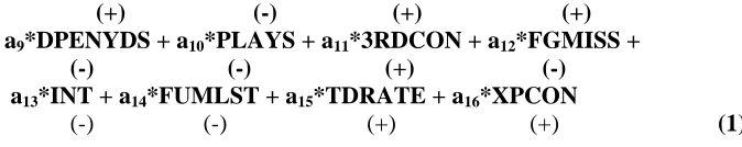
OFFPTS = aik + a1*DKO + a2*DPUNTS + a3*DFGMISS + a4*DINT +
(+) (+) (+) (+) a5* DFUMLST + a6*START + a7*OFFYDS + a8*PENYDS +
(+) (-) (+) (+) a9*DPENYDS + a10*PLAYS + a11*3RDCON + a12*FGMISS +
(-) (-) (+) (-)
a13*INT + a14*FUMLST + a15*TDRATE + a16*XPCON
[image:8.612.160.497.73.140.2](-) (-) (+) (+) (1)
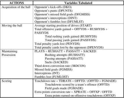
Table One separates the independent variables into four separate actions:
Acquisition of the Ball, Moving the Ball, Maintaining Possession, and Scoring. Of the
sixteen independent variables that comprise these actions, we are most interested in Total
Offensive Yards Gained (OFFYDS). This factor, listed under Moving the Ball, is calculated
by adding rushing (RUSHYDS) and passing yards (PASSYDS) together.
It is possible that rushing and passing yards have differing impacts on scoring, and
before we discuss the economic returns to these actions the value of rushing and receiving
on the field has to be ascertained. Consequently equation (1) was estimated with OFFYDS
separated into RUSHYDS and PASSYDS. The results are reported in Table 1b.
Berri (2007) reported that each additional OFFYDS increased scoring by 0.08, or 100
additional yards would lead to 7.96 additional points. From Table Two we see that each
additional RUSHYDS and PASSYDS also lead to 0.08 points. When we compare 100
RUSHYDS to 100 PASSYDS, we see that the former generates 8.30 points while the latter
creates 7.85 points.
Although the coefficients on RUSHYDS and PASSYDS are virtually the same, a
case can still be made for the proposition that the returns to receiving are higher than the
returns to rushing. In order to acquire yards a running back must expend a Play. Table 1b
indicates that each Play, holding all else constant, costs a team -0.021 points. Looking at a
sample of running backs that had at least 100 rushing attempts in a season from 1994 to
2006, we can see that the average back gains 4.08 yards per rushing attempt but 7.93 yards
to rush 24.5 times, at a cost of 5.17 points. To gain 100 yards receiving, though, would only
require 12.61 receptions at a cost of 2.66 points. When we add together the points from
yards gained to the cost of the plays, we see that 100 rushing yards produce 3.13 points while
100 yards receiving generate 5.19 points. Hence, team returns to pass reception yards are
greater than team returns to rush yards.
3. Economic Returns to Receiving and Running
Looking at our model of scoring it does appear that the yards a running back gains
via rushing or receiving have somewhat different impacts on the field of play. Are these
yards treated differently in the marketplace? To answer this question we turn to a model of
player salaries.
The salary model
The model of player salaries used here follows the generic Mincer form in the sports
literature where player salary is assumed to depend on experience, player performance and
team characteristics (see Scully (1974) and Krautmann (1999) for baseball, Bodvarsson and
Partridge (2001), Hamilton (1997) and Kahn and Shah (2005) for basketball, Berri and
Simmons (2007) and Kahn (1992) for NFL, Idson and Kahane (2000) for hockey and
Lucifora and Simmons (2003) for Italian soccer).
Our dependent variable is player salaries. We should note that in the NFL there are
multiple measures of salary.2 The basic salary is paid conditional on appearances and is not
guaranteed. In addition there is often a signing bonus, which is a lump-sum payment to the
player that is guaranteed and averaged over the duration of a player’s contract for purposes
performance, although we should note that these bonuses tend to be small compared to the
signing bonus.
Basic salary levels are set within a pay scale determined by collective bargaining
agreement between the players’ association (NFLPA) and team owners.3 The pay scales will
reflect player experience in the NFL. Signing bonuses are determined through bilateral
bargaining between team owners and the player without union involvement. In any season, it
follows that the variation in signing bonus will be somewhat larger than the variation in basic
salary. Over our sample period, it appears that an increasing share of total player salary is
accounted for by signing bonuses. For the purposes of salary cap computation, any signing
bonuses are pro-rated over the life of the player’s contract and the measure of salary that we
will use is:
Salary = Base salary + Pro-rated signing bonus + Other bonuses
Salary distributions in most occupations are not log-normal and in team sports,
skewness in the distribution is particularly marked with a few top players earning
substantially more than their colleagues (Lucifora and Simmons, 2003). Non-normality and
skewness in the dependent variable may result in variations of marginal returns to particular
characteristics throughout the salary distribution (Leeds and Kowalewski, 2001).
We are particularly concerned with a comparison of returns to different performance
measures. Since these returns are likely to vary through the salary distribution -- and as our
data cover 12 NFL seasons -- we need to deflate total salary by an appropriate measure to
2
Salary data is provided by USA Today and Rod Fort’s Sports Business web site, www.rodneyfort.com/SportsData.
3
obtain real values. We need to do this so that a given position in the salary distribution of
running backs in 1995 is similar to the same part of the distribution in 2005.
The rate of NFL salary inflation has been considerably in excess of consumer price
inflation over our sample period of 1995 to 2006. Rather than deflate salaries by price
inflation we scale salaries of running backs by average NFL salary in each season. The
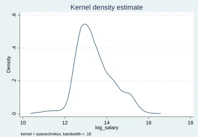
resulting values of log real salary are clearly not log-normal, as can be seen in the kernel
density plot shown in Figure 1. For our sample of 1,425 player-seasons we find a kurtosis
value of 3.24. Since this value exceeds 3, we have excess kurtosis and we are reluctant to
proceed with ordinary least squares estimation for our model.4
With dependent variable described, we move on to a discussion of our independent
variables. And this list of variables begins with player experience. We measure experience as
the number of accumulated seasons’ active performance in the NFL (Experience). If a player
misses a season due to injury or contract hold-out this season is not counted as experience.5
As with the human capital model, we expect NFL experience to impact player salaries
positively6 but with diminishing returns to reflect the wear and tear on the body and decline
in physical ability (speed and strength) that is clearly apparent in playing careers that average
just four years in this highly physical sport. Diminishing returns to experience are captured
by a quadratic form with the addition of Experience squared.
the distribution of team payrolls in NFL is more compressed than in other North American sports and the salary cap can be viewed as binding.
4
If salaries are deflated by CPI, the kurtosis value becomes 3.84, suggesting an even stronger departure from log-normality in the dependent variable.
5Player records were taken from Carroll et al. (1999) and various editions of the NFL Fact and Record Book.
6
NFL experience for most players – at least in our sample – is preceded by the
league’s player draft. There are 12 draft rounds and players drafted in earlier rounds tend to
be of higher quality than players drafted in later rounds. Hence, earlier round choices should
have greater salaries. Also, players selected in earlier rounds will receive greater technical and
coaching support than players selected in later rounds so the prediction that these players
will earn larger salaries is partly self-fulfilling.
We should note that the draft is an imperfect predictor of playing talent, especially as
teams use the draft partly as a trading exchange for players (Hendricks et al. 2003, Quinn
(2006)).7 Kahn (1992) used the inverse of draft round as a control variable in models of NFL
player salary to capture the non-linearity in impact of draft round number on player salary.
We experimented with this specification and with a set of dummy variables for draft round
and found that only rounds one and two significantly affected salary. Hence, we retain Draft
round 1 and Draft round 2 as dummy variables to reflect draft choices. We assume that once
achieved, high draft status remains an influence on player salary throughout the player’s
career.
Players with three years experience in the NFL are entitled to ‘restricted free agency’.
After three years, a player can seek contract offers from rival teams but the current team is
entitled to present a matching offer. Such players are denoted by the dummy variable,
Restricted free agent.
NFL players are entitled to unfettered free agency status after four seasons playing
experience. Players who have at least four years experience are denoted by the dummy
variable Veteran. Several players remained with their drafting team even though they had
acquired free agent status. This is presumably because the drafting team offered the player a
contract with valuation at least as high as any alternative offer by another team in the market
for free agents. Such players who remain with their original drafting teams despite being free
agents are denoted by the dummy variable Stayer. This is set at one until the player switches
teams. We predict that both ‘veterans’ and ‘stayers’ will earn higher salaries than players who
do not have free agent status (see Krautmann et al. 2007 for a full account of conditions for
free agency in NFL).
Inspection of our data suggests that players often receive lower salary when they
change teams. We capture this effect by a dummy variable, Change team, where the value of
unity only applies for the first season in which a player represents a different club. This
variable was found to be negative and significant in the analysis of NFL quarterback salaries
of Berri and Simmons (2005). Their rationale was that teams which identified an effective
job match with their quarterbacks would offer salaries in excess of outside opportunities,
even for free agents. Players who switch teams would then tend to be those deemed surplus
to requirements. We anticipate a similar effect for running backs.
Berri and Simmons (2005) also identified appearance in the annual Pro Bowl
exhibition game as an indicator of player value. In their model of NFL quarterback salaries,
players who had at any time previously appeared in the Pro Bowl received higher salaries
ceteris paribus and we expect the same result for running backs. The dummy variable for Pro
Bowl appearance is denoted by Pro bowl.
Although characteristics unique to the players are important, we must remember that
football is a team game. Specifically, this is an interactive team game with complementarity
7
between team inputs.8 Modeling this complementarity is still in its infancy in the sports
economics literature (Borland, 2006). One promising attempt was by Idson and Kahane
(2000) for the National Hockey League. They extracted measures of team-mate performance
minus the performance of a given player in their data set, for the same performance variable.
Unfortunately, not all NFL players have directly observable performance metrics and
this is particularly the case for players on the offensive line. These players block defensive
players in an effort to give skill players the time and space necessary to move the ball.
Statistics for offensive line players, though, are somewhat scarce and not independent fo the
numbers tracked for running backs and quarterbacks. Still, we can proxy the quality of the
offensive line by noting the total salary of this unit on the team.
In a competitive labor market, offensive line payroll would be an extremely good
proxy for the overall quality of the offensive line. Unfortunately, the NFL labor market is
restrictive and, with just 32 teams, monopsonistic. Players who are not free agents tend to
receive salaries below marginal revenue product (Krautmann et al. 2007) and as a result the
relationship between team performance and team payrolls is expected to be weak.9
Consequently, the relationship between payroll and latent performance of the offensive line
is bound to be imperfect. Despite the problems associated with our measure, we expect a
better (more expensive) offensive line should present running backs with improved
opportunities to gain yards and should hence raise their productivity and salaries. We use the
log of offensive line salary, to include all offensive line players on a team’s roster in a given
season, again deflated by average NFL salary.
8
The same can be said of all major sports, although separation of production inputs is more apparent in baseball.
Similarly, offense salary is the log of total salaries of all ‘skill’ players on a team’s roster
minus the salary given running back in any observation, deflated by average NFL salary. By
skill players, we mean quarterbacks, wide receivers, tight ends and other running backs. We
predict complementarity between offensive line and running backs in team production and
hence a positive coefficient on offensive line salary. Similar complementarity could well exist
between skill players and the running back in any observation but an opposing effect may
occur through the salary cap. Extra salary to other skill players takes a team closer to its cap
and may necessitate a cut in salary for a given running back. Consequently, the sign of
coefficient on offense salary will then be ambiguous.
We retain one further team characteristic which is market size. This is proxied by the
log of SMSA population (Population). It might be argued that teams in larger markets (New
York Giants and Jets) can afford to pay higher salaries than teams in smaller markets
(Kansas City Chiefs and Green Bay Packers). As noted above, the NFL does have a binding
salary cap that is designed to prevent this outcome. This cap is also reinforced by extensive
revenue sharing of both gate and broadcast revenues. If effective, these measures should
serve to reduce the impact of market size on team revenues and hence on individual pay.
We have now listed all of the individual and player characteristics we suspect impacts
salary, except the specific actions running backs take on the field of play. At the onset we
noted that running backs have three defined tasks: rushing, receiving, and blocking.
Although most running backs focus on at least one of the first two tasks, there are some
running backs – called full backs – that have blocking as their primary function. These backs
typically perform relatively little ball carrying or pass receiving and are generally taller and
We also examine impacts of interaction terms between full back and our performance
measures.
Turning to our performance measures, we begin by noting that we examined the set
of performance measures tracked for running backs and found that the indicator which
dominated all others in predicting player salaries was yards achieved, as opposed to rushing
attempts, touchdowns, or fumbles. When it comes to examining yards, we made a few
distinctions. First, we predict that players with established career performance will be
rewarded with higher salaries than those who lack sustained performance. Consequently, our
list of performance measures begins with total career rushing yards (Career rush yards) and
total career pass reception yards (Career receiving yards) up to and including two seasons before
the time player salary was determined.
Although career performance is important, we also expect that what a player did
most recently to matter as well. Specifically, since total salary is determined before the
season in question, we expect that what transpired the previous season to be significant.
Hence we include Rush yards (t-1) and Receiving yards (t-1)as our key performance metrics for
running backs.
We are not simply interested in the returns to rushing and receiving. Our test for
specialization of running backs uses the interaction term Receiving yards*Rush yards. The sign
of coefficient on this term offers insight into whether or not specialization raises running
back salary. If pass reception yards and rush yards are complements in salary determination
we would predict the coefficient on the interaction term to be positive. This would suggest
salary gains from versatility. A negative coefficient suggests that an increase in one measure
of player performance reduces the marginal salary returns of the other measure. Hence, an
The implication is that running backs would be better off in salary from specialization in
either pass receptions or rushing.
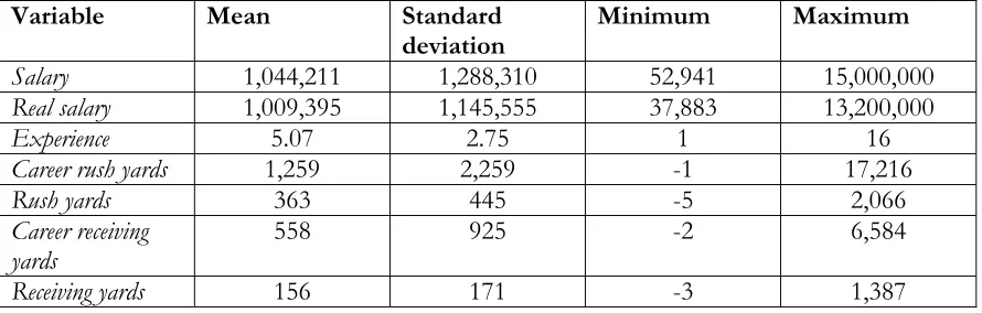
Our sample consists of running backs who made at least one play (rush attempt or
pass reception) in the previous season, yielding 1,423 player-season observations from 624
running backs. Table 2 reports some descriptive statistics for continuous measures of salary,
experience and performance. To summarize, our salary model is:
Log salary = F(Experience, Experience squared, Draft round 1, Draft round 2, Veteran, Stayer,
Restricted free agent, Change team, Offensive line salary, Offense salary, Pro Bowl, Population, Full back,
Career rush yards, Career receiving yards, Rush yards, Receiving yards, Receiving yards*Rush yards)
As with Berri and Simmons (2005), and following earlier contributions by Hamilton
(1997) and Leeds and Kowalewski (2001), we adopt the quantile regression method for
estimation since salaries have a non-normal distribution with substantial skewness and excess
kurtosis.10 At the median, quantile regression differs from ordinary least squares in that it
minimizes the sum of absolute residuals rather than the sum of squared residuals (Koenker,
2005). A strong advantage of quantile regression is that it permits estimation of marginal
effects of covariates at different points of the distribution of the dependent variable. In our
case, we can estimate the impacts of player performance measures on log salary at different
salary quantiles. The selected quantiles for estimation are 0.1, 0.25, 0.5 (median), 0.75 and 0.9
and results are reported in Table 2a. Quantiles are estimated simultaneously and standard
10
errors are bootstrapped with 200 replications.11 For comparison, we also show results from
Huber robust or trimmed regression which is a weighted least squares estimator that adjusts
the regression for the influence of outliers. Again, this method is designed to address the
non-normality inherent in the dependent variable. These additional results are shown in
Table 2b.
Results
The estimation of our salary model is reported in Tables 3 and 4. Although our
focus is on the returns to rushing and receiving, we begin our discussion with the impact of
our control variables. In Tables 3a and 3b the control variables generally have significant
coefficients with signs as predicted. The median quantile regression model and the Huber
regression model each deliver significant coefficients on all covariates except for Population
and offense salary. The results with respect to the former indicate that there is no support for
the hypothesis that teams with bigger local populations and hence market size pay higher
salaries to running backs.12
Our discussion of the statistically significant control variables begins with experience.
The turning point on Experience for the median regression is 6.8 years. With a typical drafting
age from college of 21 or 22, this corresponds to an age level that maximizes salary of 28 or
29, a figure that is consistent with findings from other sports leagues (e.g. Lucifora and
Simmons, 2003 for Italian soccer and Turner and Hakes, 2007, for Major League Baseball).
As explained previously, NFL experience is preceded by the draft. Consistent with
our expectation, the impact on being picked in round 2 of the draft is generally greater than
for later rounds but less than for round 1. Veteran players gain a salary premium at the
11
median above. In the bottom half of the salary distribution, there is no premium. This
suggests that free agency per se does not raise salary; free agency must be accompanied by
requisite ability.
The nature of free agency also matters. Restricted free agents earn a premium from
the 0.25 quantile upward. The similarity of coefficient values of veteran and restricted free agent
from median upwards suggests that franchises anticipate full free agent status of high ability
players by rewarding them even after three years. Players who stay with their original team
beyond free agency entitlement earn an additional premium compared to veterans who
move. In fact, players who change team suffer an immediate salary reduction.
Beyond free agency, we find that players who gain Pro Bowl appearances receive
increments to salary over and above performance and these are sustained for the full
duration of their careers. In addition, full backs -- who tend to block rather than run with or
receive the ball -- gain a salary premium as reward for their skills that are less well-observed
(to the econometrician). This premium varies from 7.1 per cent at the 0.75 quantile to 11.4
per cent at the 0.1 quantile, although is insignificantly different from zero at the 0.90
quantile.
The importance of blocking is not only seen with respect to fullbacks. Specifically, at
the 0.10 quantile, the coefficients of offense salary and offensive line salary are each significantly
different from zero at the five per cent level. Beyond this quantile, however, only offensive line
salary has significant coefficients. We interpret this as indicative of complementarity between
the productivities of the offensive line and running backs. In essence, the quality of the
offensive line blocking for a running back appears to impact his production and value.
12
Turning to the running back’s production, we find that Career rush yards are a
significant predictor of salary throughout the distribution (at 10 per cent significance or
better). The significance of career receiving yards, however, is not apparent at the 0.75 and
0.90 quantiles. Below these quantiles, the impact of 100 extra career receiving yards is
significantly greater than the impact of 100 extra career rushing yards.
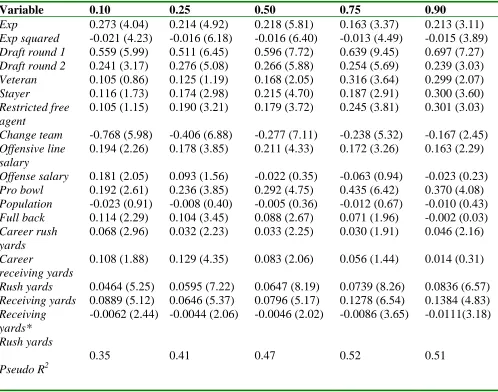
To assess the impacts of specialization on salary, we turn to our focus variables, Rush
yards, Receiving yards and Receiving yards*Rush yards. The coefficients on Rush yards and Receiving
yards are significant and positive at all estimated quantiles. Moreover, the impacts are greater
at quantiles above the median compared to below. 13The interaction term Receiving yards*Rush
yards has a significant (at five per cent at least), negative coefficient at all estimated quantiles.
Hence, the marginal salary returns to extra receiving yards declines with extra rush yards.
Equivalently, the marginal salary returns to extra rushing yards declines with extra receiving
yards. This is indicative of gains from specialization in either skill performed by NFL
running backs.
Our results show that the marginal salary returns to one skill depend negatively on
the performance level observed for the other skill. Although our results are statistically
significant, it is important to also consider economic significance. Specifically, we wish to
consider how the coefficients reported in Table 3a convert into predicted estimates of salary
returns at different quantiles of the salary distribution.
Table 4 offers a simulation of these predicted returns, holding control variables and
career rush and receiving yards constant. This permits a focus on the immediate impacts of
100 extra yards rushing or receiving. The values of rush yards and receiving yards shown in
quantile. The neighborhood is just above the preceding quintile and just below the next
quantile to be estimated. Where positive, the estimated marginal returns are over and above
the NFL league average salary increase for a particular season. Where negative, marginal
salary returns are lower than the NFL league average, but do not necessarily imply salary
reduction.
For example, consider three running backs, each at the median of the salary
distribution and each with control variables (Experience, Offensive line salary, etc...).
Additionally, each has the same value for career rush and receiving yards. Imagine, though,
that we now observe differences with respect to Rush yards and Receiving yards. Running back
A has become a rushing specialist with 900 rush yards from the previous season and zero
receiving yards. His return to 100 extra rush yards is estimated as 6.47%. His return to 100
extra receiving yards is 3.83%. Running back B is now a receiving specialist with 800 pass
reception yards in the previous season. His predicted marginal return to 100 extra receiving
yards is 7.96%. Running back C is multi-skilled; he runs with the ball and receives passes.
Suppose his previous season performance levels are 300 yards in receiving and 600 yards
rushing. The predicted marginal returns to 100 extra rush yards and 100 extra receiving yards
for Player C are 4.63% and 5.20%, respectively. For the multi-skilled player, therefore, there
is little difference in marginal returns from extra performance in either skill, at the median.
But the rewards to versatility are less than the rewards to specialization; running back C’s
marginal returns are dominated both by the larger returns to extra rush yards for the
specialist rusher and by the larger returns to extra receiving yards for the specialist pass
receiver.
13
Moving up the salary distribution, we see greater disparities between marginal returns of
the versatile players and the specialists. Consider the simulated returns at the 90th percentile
in Table 4. A player that specializes in rushing with 1,700 yards rushing and zero pass
reception yards gains a predicted marginal salary return of 8.36%. However, if this player has
100 extra yards pass reception and no extra rush yards, the marginal salary return is -5.03%.
A receiving specialist with 1,300 pass reception yards and 200 rush yards in the previous
season, derives a predicted return of 11.62% from 100 extra receiving yards but a much
lower return, -6.07%, from 100 extra rush yards. A more versatile player with 700 yards
rushing and 600 yards pass receptions would generate marginal returns of 1.70% from 100
extra rush yards and 6.07% from 100 extra receiving yards. At the 90th percentile, it appears
from our simulation that the marginal returns to specialists from extra performance levels in
the specialized skill exceed the returns to versatile players from extra performance levels in
either of their key skills. Similar disparities can be derived from our simulation of estimates
of log salary at the 75th percentile.
At 75th and 90th percentiles, the difference in marginal returns between specialist and
versatile players has widened compared with estimates at lower quantiles. Of course, this is
partly due to the fact that expected performance levels are greater at higher quantiles of the
salary distribution. Consequently this makes the downward impact of our interaction term
larger for a given coefficient. But the coefficients on the interaction term are also greater in
absolute magnitude at 75th and 90th percentiles compared to lower quantiles. These two
effects combine to deliver the disparities in marginal returns shown in Table 4.14
14
Simulations are illuminating, but let us return to the specific cases of Barry Sanders
and Marshall Faulk. Both players are in our data set. As noted in the introduction, Sanders
can be regarded as a running specialist while Faulk is a more versatile player. Due to the
scaling of nominal salary by NFL average wage, both players appear near (actually above) the
90th percentile of the salary distribution, even though Sanders exits our sample in 1998 while
Faulk first appears in our sample in 1995.
Our examination of these players will take as starting values of rush yards and
receiving yards to be 1883 and 283, respectively, for Sanders (his 1995 values) and 1,381 and
1,048 for Faulk (his 2000 values). Our simulation at the 90th percentile shows returns to 100
extra yards rushing and receiving for Sanders to be 5.22% and -7.06%, respectively. In
contrast, the comparable returns for Faulk are estimated as -3.27% and -1.49%. The
specialist has greater returns from his particular skill of rushing compared both to the
secondary skill of catching passes. Also, he generates greater returns to specialization
compared to versatility. Actually, even allowing for the full impact on career values, Faulk
would still have a greater pecuniary incentive to develop a specialty with respect to pass
receptions rather than maintain his capability with respect to both aspects of running back
performance.
In section 2, we showed that rushing yards and pass yards had virtually the same
impact on a team’s offensive performance. The similar impact of rushing and passing on
team production is not reflected in determination of running back salaries. The two findings
can be reconciled that rushing yard and receiving yard totals are achieved by a mix of players
and skills; within the running back category, there is considerable heterogeneity of talent.
This makes specialist activity possible within the position. Teams can employ one set of
running backs as pass reception specialists and another set as rushing specialists. A third set,
full backs, is used as blocking specialists.
The higher marginal returns to receiving yards over rush yards in Table 4 are
consistent with the higher team returns to pass yards over rush yards that we found in
section 2 above. Receiving yards have a larger impact on team outcomes and this is reflected
in both marginal revenue products of running backs with respect to the two performance
indicators and differentials in salary returns.
4. Conclusion
In the NFL, we observe players with well-defined tasks and precise performance
measures. This facilitates an econometric investigation of salary returns to players in the
‘skill’ position of running back. We were able to test for returns to specialization by
distinguishing between returns to pass reception yards and returns to running yards. For this
group of players, total yards achieved in a season is found to be the most fundamental
performance measure that drives player salaries.
In professional team sports, the distribution of salaries exhibits greater skewness and
kurtosis than in regular occupations. The use of quantile regression helps overcome
problems of non-normality of the dependent variable. This estimation method also permits a
flexible empirical specification in which impacts of focus variables vary through the salary
distribution.
Our analysis controls for a number of relevant covariates, including experience, draft
position on entry to the NFL, free agent status and reputation proxied by appearance in a
Pro Bowl. Going beyond previous studies of NFL salaries, we were able to control for team
complementarity by using positional payroll as a proxy for quality of team units, in particular
offensive linemen, which augment the performance and productivity of running backs. The
estimated impacts of these covariates appear plausible.
Our main finding is that there are pronounced gains to specialization for running backs,
particularly at the top end of the salary distribution. We find that the marginal returns to
receiving (rush) yards falls with extra rush (receiving) yards. The coefficient on the
interaction term between receiving yards and rush yards is negative and significant at all
estimated quantiles. When we simulate the model, we find substantial predicted differences
in returns from receiving and rush yards as between specialists and versatile players. Again,
these differences are more pronounced at the 75th and 90th percentiles.
Having set out the case for specialization, our analysis could be usefully improved in a
number of ways in future work. First, we have not explicitly modeled career duration.
Running backs that specialize in pass receptions may be less prone to serious knee injuries
that plague specialist rushers. A hazard analysis could complement the findings presented
here although we should caution that several players in our sample have short careers of
three years or less. Second, we have not fully captured variations in playing styles between
teams and seasons. These variations are largely attributable to the preferences of particular
head coaches. Some head coaches are more oriented towards a running game than others.
Future work would usefully attempt to identify the impact of head coach strategies on
References
Bardasi, Elena and Mark Taylor. 2007. Marriage and wages: A test of the specialization
hypothesis. Economica, forthcoming.
Baron, John and David Kreps. 1999. Strategic Human Resources: Frameworks for General Managers,
John Wiley.
Berri, David J.(2007). Back to Back Evaluation on the Gridiron. In Statistical Thinking in Sport,
eds. James H. Albert and Ruud H. Koning, Chapman & Hall/CRC: 235-256.
Berri, David J., Martin B. Schmidt and Stacey L. Brook. 2006. The Wages of Wins. Stanford
Business Press.
Berri, David J. and Rob Simmons. 2005. Race and the Evaluation of Signal Callers in the
National Football League. Lancaster University Management School Discussion Paper.
Black, Sandra E. and Lisa M. Lynch. 2004. “What’s Driving the New Economy?: The
Benefits of Workplace Innovation.” Economic Journal, 114: F97- F116.
Bodvarsson, Orn B. and Mark D. Partridge. 2001. “A Supply and Demand Model of
Co-Worker, Employer and Customer Discrimination.” Labour Economics, 8: 389-416.
Borland, Jeffrey. 2006. “Production functions for sporting teams.” In Wladimir Andreff and
Stefan Szymanski (eds.) Handbook on the Economics of Sport, 610-615. Cheltenham:Edward
Elgar.
Carmichael, H. Lorne and W. Bentley MacLeod. 1993. “Multiskilling, Technical Change and
the Japanese Firm.” Economic Journal, 103: 142-160.
Carroll, Bob, Michael Gershman, David Neft and John Thorn. 1999. Total Football II: The
Official Encyclopedia of the National Football League. New York: Harper Collins.
Garicano, Luis and Thomas N. Hubbard. 2007. “Managerial Leverage is Limited by the
Extent of the Market: Hierarchies, Specialization and the Utilization of Lawyers’ Human
Capital.” Journal of Law and Economics. 50: 1-43.
Green, Francis, Stephen Machin and David Wilkinson. 1998. “The Meaning and
Determinants of Skill Shortages.” Oxford Bulletin of Economics and Statistics. 60: 167-185.
Hamilton, Barton H. 1997. “Racial Discrimination and Professional Basketball Salaries in the
1990s.” Applied Economics. 29: 287-296.
Hendricks, Wallace, Lawrence DeBrock and Roger Koenker. 2003. “Uncertainty, Hiring and
Subsequent Performance: The NFL Draft.” Journal of Labor Economics. 21: 857-886.
Ichniowski, Casey and Kathryn Shaw. 2003, “Beyond Incentive Pay: Insiders’ Estimates of
the Value of Complementary Human Resource Management Practices.” Journal of Economic
Perspectives. 155-180.
Idson, Todd L. and Leo H. Kahane. 2000. “Team Effects on Compensation: An Application
to Salary Determination in the National Hockey League.” Economic Inquiry. 38: 345-357.
Kahn, Lawrence M. 1992. “The Effects of Race on Professional Footballers’
Compensation.” Industrial and Labor Relations Review. 45: 295-310.
Kahn, Lawrence M. 2000. “Sports as a Labor Market Laboratory.” Journal of Economic
Perspectives. 14: 75-94.
Kahn, Lawrence M. and Malav Shah. 2005. “Race, Compensation and Contract Length in
the NBA: 2001-2002.” Industrial Relations. 44: 444-462.
Koenker, Roger. (2005). Quantile Regression. Cambridge: Cambridge University Press.
Krautmann, Anthony. 1999. “What’s Wrong with Scully-Estimates of a Player’s Marginal
Krautmann, Anthony, Peter von Allmen and David J.Berri. 2007. “The Underpayment of
Restricted Players in North American Sports Leagues.” Presented at Western Economic
Association International Conference, Seattle.
Leeds, Michael and Kowalewski, Sandra. 2001. “Winner Take All in the NFL: The Effect\of
the Salary Cap and Free Agency on the Compensation of Skill Position Players.” Journal of
Sports Economics. 2: 244-256.
Lucifora, Claudio and Rob Simmons. 2003. “Superstar Effects in Sport: Evidence from
Italian Soccer.” Journal of Sports Economics. 4: 35-55.
The NFL Record & Fact Book. Various Editions.
Quinn, Kevin G. 2006. “Who Should be Drafted? Predicting Future Professional
Productivity of Amateur Players Seeking to Enter the National Football League.”,
St.Norbert College, mimeo.
Scully, Gerard W. 1974. “Pay and Performance in Major League Baseball.”American Economic
Review. 64: 915-930.
Simmons, Rob and David Forrest. 2004. “Buying Success: Team Performance and Wage
Bills in U.S. and European Sports Leagues.” In Rodney Fort and John Fizel (eds.)
International Sports Economics Comparisons, 123-140. Westport,CT: Praeger.
Stigler, George. 1951. “The Division of Labor is Limited by the Extent of the
Market.”Journal of Political Economy. 59: 185-193.
Turner, Chad and Jahn Hakes. 2007. “Pay, productivity and aging in Major League Baseball.”
Figure 1
Kernel density plot of log salary
0
.2
.4
.6
De
n
s
it
y
10 12 14 16 18
log_salary
kernel = epanechnikov, bandwidth = .18
Table 1a
Factors Impacting a Team’s Offensive Ability
ACTIONS Variables Tabulated
Acquisition of the ball Opponent’s kick-offs (DKO) Opponent’s punts (DPUNTS)
Opponent’s missed field goals (DFGMISS) Opponent’s interceptions (DINT)
Opponent’s fumbles lost (DFUMLST) Moving the ball Average starting position of drives (START)
Total offensive yards gained = OFFYDS = RUSHYDS + PASSYDS
Total rushing yards gained (RUSHYDS) Total passing yards gained (PASSYDS) Total penalty yards lost (PENYDS)
Total penalty yards lost by the opponent (DPENYDS) Maintaining
Possession
PLAYS = RUSHATT + PASSATT + SACKED Rushing attempts (RUSHATT)
Passing attempts (PASSATT) Sacks (SACKED)
Third down conversion rate (3RDCON) Missed field goals (FGMISS)
Interceptions (INT) Fumbles lost (FUMLOST)
Scoring Touchdown rate = TDRATE = OFFTD / (OFFTD + FGMADE)
Touchdowns scored by a team’s offence (OFFTD) Field goals made (FGMADE)
Table 1b
Modeling Offensive Scoring
Dependent Variable: Offensive Points Scored (OFFPTS)
Team Fixed Effects and Dummy Variables for each season were employed.
Variable Label Coefficient t-Statistic
Opponent's Kick-offs DKO* 0.93 3.67
Opponent's Punts DPUNTS** 0.43 2.12
Opponent's Missed Field Goals DFGMISS 0.48 0.82
Opponent's Interceptions Thrown DINT* 1.26 4.28
Opponent's Fumbles Lost DFUMLST** 1.01 2.49
Average Starting Position of Drives START* 10.03 11.17
Yards Gained, Rushing RUSHYDS* 0.08 13.46
Yards Gained, Passing PASSYDS* 0.08 17.98
Penalty Yards PENYDS -0.01 -1.21
Opponent's Penalty Yards DPENYDS* 0.06 5.02
Plays PLAYS* -0.21 -4.12
Third Down Conversion Rate 3RDCON* 1.91 3.93
Field Goals Missed FGMISS* -3.00 -5.35
Interceptions Thrown INT* -1.29 -3.49
Fumbles Lost FUMLST* -1.49 -3.56
Percentage of Scores that are Touchdowns TDRATE* 101.56 4.46
Extra Point Conversion Rate XPCON 44.07 1.58
Adjusted R-squared 0.910
Observations 251
Note: The data utilized to estimate this model came from various issues of the Official National Football League Record & Fact Book. The lone exception is START, which was taken from Football Outsiders.com.
Table 2
Descriptive statistics for continuous salary, experience and performance variables
Variable Mean Standard
deviation Minimum Maximum
Salary 1,044,211 1,288,310 52,941 15,000,000
Real salary 1,009,395 1,145,555 37,883 13,200,000
Experience 5.07 2.75 1 16
Career rush yards 1,259 2,259 -1 17,216
Rush yards 363 445 -5 2,066
Career receiving
yards 558 925 -2 6,584
Table 3a
Quantile Regression Results
Dependent variable is log real salary for running backs with positive plays in previous season; sample period 1995-2006; N = 1423
Variable 0.10 0.25 0.50 0.75 0.90
Exp
Exp squared Draft round 1 Draft round 2 Veteran Stayer Restricted free agent Change team Offensive line salary Offense salary Pro bowl Population Full back Career rush yards Career receiving yards Rush yards Receiving yards Receiving yards* Rush yards
Pseudo R2
0.273 (4.04) -0.021 (4.23) 0.559 (5.99) 0.241 (3.17) 0.105 (0.86) 0.116 (1.73) 0.105 (1.15) -0.768 (5.98) 0.194 (2.26) 0.181 (2.05) 0.192 (2.61) -0.023 (0.91) 0.114 (2.29) 0.068 (2.96) 0.108 (1.88) 0.0464 (5.25) 0.0889 (5.12) -0.0062 (2.44) 0.35 0.214 (4.92) -0.016 (6.18) 0.511 (6.45) 0.276 (5.08) 0.125 (1.19) 0.174 (2.98) 0.190 (3.21) -0.406 (6.88) 0.178 (3.85) 0.093 (1.56) 0.236 (3.85) -0.008 (0.40) 0.104 (3.45) 0.032 (2.23) 0.129 (4.35) 0.0595 (7.22) 0.0646 (5.37) -0.0044 (2.06) 0.41 0.218 (5.81) -0.016 (6.40) 0.596 (7.72) 0.266 (5.88) 0.168 (2.05) 0.215 (4.70) 0.179 (3.72) -0.277 (7.11) 0.211 (4.33) -0.022 (0.35) 0.292 (4.75) -0.005 (0.36) 0.088 (2.67) 0.033 (2.25) 0.083 (2.06) 0.0647 (8.19) 0.0796 (5.17) -0.0046 (2.02) 0.47 0.163 (3.37) -0.013 (4.49) 0.639 (9.45) 0.254 (5.69) 0.316 (3.64) 0.187 (2.91) 0.245 (3.81) -0.238 (5.32) 0.172 (3.26) -0.063 (0.94) 0.435 (6.42) -0.012 (0.67) 0.071 (1.96) 0.030 (1.91) 0.056 (1.44) 0.0739 (8.26) 0.1278 (6.54) -0.0086 (3.65) 0.52 0.213 (3.11) -0.015 (3.89) 0.697 (7.27) 0.239 (3.03) 0.299 (2.07) 0.300 (3.60) 0.301 (3.03) -0.167 (2.45) 0.163 (2.29) -0.023 (0.23) 0.370 (4.08) -0.010 (0.43) -0.002 (0.03) 0.046 (2.16) 0.014 (0.31) 0.0836 (6.57) 0.1384 (4.83) -0.0111(3.18) 0.51
Note: t statistics are computed using bootstrapped standard errors with 200 replications.
Table 3b
Robust regression results
Variable Coefficient (t statistic)
Exp
Table 4
Percentage returns to 100 yards extra rush yards (x) or 100 yards extra pass yards (y): Cells denote x,y
10% quantile
Log salary = 0.0464*Rush yards + 0.0889*Receiving yards – 0.0062*Receiving yards*Rush yards
Rush yards Receiving
yards
0 150 400 600 1300
0 4.64,7.96 4.64,6.41 4.64,5.17 4.64,0.83
100 4.02,8.89 4.02,7.96 4.02,6.41 4.02,5.17 4.02,1.79 200 3.40,8.89 3.40,7.96 3.40,6.41 3.40,5.17 3.40,1.79 300 2.78,8.89 2.78,7.96 2.78,6.41 2.78,5.17 2.78,1.79 400 2.16,8.89 2.16,7.96 2.16,6.41 2.16,5.17 2.16,1.79
25% quantile
Log salary = 0.0595*Rush yards + 0.0646*Receiving yards – 0.0044*Receiving yards*Rush yards
Rush yards Receiving
yards
0 200 500 800 1500
0 5.95,5.58 5.95,4.26 5.95,2.94 5.95,-0.14
100 5.51,6.46 5.51,5.58 5.51,4.26 5.51,2.94 5.51,-0.14 200 5.07,6.46 5.07,5.58 5,07,4.26 5.07,2.94 5.07,-0.14 300 4.63,6.46 4.63,5.58 4.63,4.26 4.63,2.94 4.63,-0.14 600 3.31.6.46 3.31,5.58 3.31,4.26 3.31,2.94 3.31,-0.14
Median
Log salary = 0.0647*Rush yards + 0.0796*Receiving yards – 0.0046*Receiving yards*Rush yards
Rush yards Receiving
yards
0 300 600 900 1700
0 6.47,6.58 6.47,5.20 6.47,3.82 6.47,0.14
75% quantile
Log salary = 0.0739*Rush yards + 0.1278*Receiving yards – 0.0086*Receiving yards*Rush yards
Rush yards Receiving
yards
0 500 900 1400 1800
0 7.39,8.48 7.39,5.04 7.39, 0.74 7.39,-2.70 200 5.67,12.78 5.67,8.48 5.67,5.04 5.67,0.74 5.67,-2.70 400 3.95,12.78 3.95,8.48 3.95,5.04 3.95,0.74 3.95,-2.70 600 2.23,12.78 2.23,8.48 2.23,5.04 2.23,0.74 2.23,-2.70 1300 -3.79,12.78 -3.79,8.48 -3.79,5.04 -3.79,0.74 -3.79,-2.70
90% quantile
Log salary = 0.0836*Rush yards + 0.1384*Receiving yards – 0.0111*Receiving yards*Rush yards
Rush yards Receiving
yards
200 700 1200 1700 2000