Learning from multiple analogies: an
Information Theoretic framework for
predicting criminal recidivism
Bhati, Avinash
2007
Online at
https://mpra.ub.uni-muenchen.de/11850/
An Information Theoretic Framework for
Predicting Criminal Recidivism
Avinash Singh Bhati
∗Paper to be presented at
the 2007 ASC Annual Meeting, Atlanta GA
Abstract
If recidivism is defined as rearrest within a finite period following lease from prison, then the kinds of outcomes typically available to re-searchers include: (i) whether or not the individual was rearrested within the follow-up period; (ii) how many times the individual was rearrested; and (iii) what was the duration from release to first (or subsequent) re-arrest. Since these outcomes are all different manifestations of the same underlying stochastic process, they provide multiple analogies from which to recover information about it. This paper develops a semi-parametric approach for utilizing information in these, and several other related out-comes, to predict criminal recidivism and presents preliminary findings.
1. OVERVIEW
The statistical analysis of criminal recidivism performs two critical functions within the field of criminal justice research. First, it is typically a key measure ∗Senior Research Associate, Justice Policy Center, The Urban Institute, 2100 M Street, NW,
Washington, DC 20037. Please do not cite without permission of the author.
used for evaluating the efficacy of crime control policy and practice (Lipton, Martinson and Wilks 1975; Sherman et al. 1997). Second, it is used almost ex-clusively as the measure with which to develop and validate actuarial risk as-sessment instruments for offender populations (Glaser 1955; Gottfredson and Gottfredson 1986). The contribution that the analysis of criminal recidivism can make to our understanding of criminal justice policy and practice, there-fore, cannot be overstated.
Criminal recidivism can best be thought of as a process that results in one or more events. Defined nominally as “the reversion of an individual to criminal behavior after he or she has been convicted of a prior offense, sentenced and (presumably) corrected” (Maltz 1984, pg 1), the empirical study of recidivism usually requires operationalizing, measuring, and modeling this concept.
The first of these components—operationalization—is informed largely by the purpose of the analysis. What do we wish to study when we analyze crimi-nal recidivism? The answer to this is theoretically motivated and typically leaves little room for an empirical analyst’s subjective interpretation; either the opera-tionalization is appropriate or is not. The second component—measurement—is a function of the availability of accurate measures of an appropriate operational-ization. Again, there is little room for analysts’ subjective assessment here; ei-ther measures are accurate or they are not. It is at the modeling stage—the last component—where an analyst confronts a crucial choice: If a process yields sev-eral manifestations, which one(s) to analyze? This seemingly innocuous choice can play a surprisingly influential role in the ensuing results.
This paper seeks to demonstrate the utility of an information theoretic frame-work for constructing and estimating semi-parametric models of criminal recidi-vism which build on the fundamental recognition that multiple manifestations of a process provide multiple analogies about it. As such, models consistent with several related analogies ought to yield keener insights into the process.
Analysis—it offers more than a marriage of these two sub-fields. It makes novel contributions to each of these sub-fields independently, while advancing the state-of-the-art in predicting criminal recidivism. Preliminary findings, using a real world data set, suggest that the analytical strategy works well in within-sample, out-of-within-sample, as well as off-the-support prediction problems.
The rest of this paper is organized as follows. The next section motivates the work and reviews the relevant literature. Following that, the information theoretic framework is described. To demostrate the potential of the analytical strategy, the paper then discusses an empirical application. As the work is ongo-ing, only preliminary findings are presented and discussed. The paper concludes with a brief discussion of the findings and enumerates promising directions for future work. Technical details are provided in a mathematical appendix.
2. MOTIVATION AND BACKGROUND
This is an unfortunate situation for the empirical analyst since these out-comes (binary, count, and duration, among others) are all different manifes-tations of the same underlying stochastic process thereby providing multiple analogies from which to recover information about it. The main motivation of this research effort is to develop and assess the utility of an information theoretic framework for incorporating information from several related manifestations— the multiple analogies—into a single model describing the stochastic process of criminal recidivism. Presumably, the more structure we can build into this model, the keener its insights will be regarding the process under study.
Scholars from most social science disciplines recognize well that event his-tory data can be presented and analyzed in numerous ways (Kalbfleisch and Prentice 1980; Allison 1982, 1984; Mayer and Tuma 1990; Lancaster 1990; Yam-aguchi 1991; Beck 1998; Box-Steffensmeier and Jones 2004). They also recognize that these seemingly disparate approaches are all connected through the underly-inghazard(failure, arrival, or event) rate. Texts or other expositional materials, for example, typically begin with an explication of the hazard rate and its various transformations—the survival rate and event probability function. Monographs covering criminal recidivism are no exception (Maltz 1984; Schmidt and Witte 1988).
To be sure, methods for including information in more than one manifes-tation of a process do exist. For example, researchers oftentimes estimate zero-inflated or hurdle models of event-counts that analyze count and binary manifes-tations of the events simultaneously (Cameron and Trivedi 1998; Greene 2000). Similarly, an impressive array of models dealing with inter-event duration de-pendence in event-count models have been invented (King 1989; Winkelmann 1995); as have methods for combining duration information in recurring failure events (Lin, Wei and Ying 1998; Ezell, Land and Cohen 2003).
This ability to incorporate information in multiple manifestations comes at a price, however. Some restrictive assumptions must be tolerated. Unfortunately, the estimation and inferential implications of these assumptions are not benign (Dean and Balshaw 1997), especially as they relate to the form of unobserved heterogeneity (Heckman and Singer 1984a,b). In order to develop and estimate models that are robust to some of these limitations—while, at the same time, able to incorporate information from multiple analogies—it would be helpful to rely less on unverifiable assumptions and more on a full utilization of all available ev-idence. Such a strategy would approach crucial aspects like proportionality and duration dependence in an agnostic fashion and be more concerned about prof-itably utilizing all available manifestations of the process. One such approach is explained next.
3. ANALYTICAL STRATEGY
off the street and are therefore not at risk of failing again).1 Let us also assume
explicitly, as is typically done implicitly, that the stochastic process we are inter-ested in studying does not change during the follow-up period. If the individual is re-arrested within the follow-up periodT, then letbdenote a binary outcome coded 1; letcdenote the number of times the individual is re-arrested; and letd
denote the duration to the first re-arrest event. If the individual is not re-arrested during this period, let each of these manifestations be set to 0. Now, define
y(t) =1[t=d] and f(t) =1[t≤min(d,T)] ∀t∈ T
where T = R
+ and 1[·] is an indicator function returning 1 if the condition
inside [·] is satisfied, else 0. Consequently, y(t) is simply a function flagging when the event actually occurs and f(t)is a function flagging when the event is at risk of occurring.2
Suppose, next, that we define r(t) as the unknown hazard that reflects the stochastic process resulting in the event flagged by y(t). Since an individual cannot fail if (s)he is not at risk of failing, we can use both y(t) and f(t) to derive conditional links between the hazard and the event as:
f(t)y(t)≈ f(t)r(t) ∀t∈ T . (1)
Besides yielding the familiar non-parametric hazard rate estimates,3this
approx-imation allows us to derive analogies between the hazard rate and several of its manifestations.
1This is for expositional purposes only. The framework may be readily adapted to account
for suchnot at riskspells, should they exist.
2By altering the definition ofy(t)and f(t)we can characterize multiple events and by
re-defining f(t)appropriately we can characterize spells when an individual is not at risk of expe-riencing the event. For ease of exposition, these nuances are omitted here.
3Assuming that the hazard is fixed across individuals, taking the unconditional expectation of
(1) and re-arranging terms yieldsˆr(t) =E[f(t)y(t)]/E[f(t)]∀t∈ T. This is a non-parametric
3.1. Identifying Suitable Analogies
First, suppose that we integrate both sides of (1) over the domainT and assume that this procedure converts the approximation into an equality. Sincey(t) =1 if and only if f(t) =1, clearly, this integration will yield the binary outcomeb
on the left hand side. Hence, this procedure yields our first analogy linking the hazard to a manifestation.
b=
Z
T
f(t)r(t)d t
Next, consider, pre-multiplying both sides of (1) by t and then taking the inte-gral. The left hand side of this equation would now yield d—the duration to first re-arrest (and 0 if the observation is censored)—since the only time when
f(t) =y(t) =1 is whent=d. Consequently, we would have identified another analogy.
d=
Z
T
t f(t)r(t)d t
Of course, there may be reason to believe that the hazard of recidivism is independently affected by a stochastic process that progresses with age (e.g., the age-crime curve). Hence, the age at first rearrest event, and not duration to first rearrest event, may be the more appropriate quantity to model. Denoting age at release as g, we definea= g+d. Multiplying both sides of (1) by a+t and integrating yields another analogy linking the hazard to age at first rearrest.
a=
Z
T
[g+t]f(t)r(t)d t
Quadratic or cibic transformation of an outcome like age at first rearrest can also be introduced in a parallel fashion.
Next, let us consider the number of rearrests within a follow-up period. If the duration to an event isηyears,4what knowledge does that provide about the
number of events likely to be accumulated through some follow-up periodT? To motivate this link, note that an increase in the duration to first re-arrest event can be expected to reduce the total number of events (rearrests) that an individual should accumulate over any fixed follow-up period. Moreover, this decrease should be proportional to the annual offending rate. Why? Because if duration to the first event increases by one year, then the total number of events that can be accumulated should be reduced by the re-arrest rate of that one year. A crude proxy for the annual offending rate, on the other hand, can be obtained by inverting the duration to first event. In other words, we can postulate the fol-lowing first order differential equation connecting the total number of rearrests to the duration to first rearrest:
d c dη=−
1
η
Solving this equation by integration yields
c = − Z 1
ηdη = −log(η) +κ
whereκis the constant of integration. Noting the terminal condition thatc=1 if η =T, we can solve for the constant of integration to get κ = 1+log(T). Reverting back to the original notation d to denote duration to first event, we can now write
c=1+logT
d.
This link betweenc andd allows us to derive another analogy. Suppose we multiply both sides of (1) by 1+log(T/t)and then integrate over the relevant domain. The left hand side would yield c and we would have derived another
analogy between the hazard and a manifestation.
c=
Z
T
[1+log(T/t)]f(t)r(t)d t
Just as age at first rearrest event could be derived from the duration variable, one can derive another analogy relating the hazard to the total number of events, since career initiation, accumulated by the end of the follow-up period. Denot-ing the number of prior (pre-release) arrests by h, the total number of arrests by follow-up as e, and multiplying bother sides of (1) by h+1+log(T/t), we obtain
e=
Z
T
[h+1+log(T/t)]f(t)r(t)d t.
In general, of course, we can derive a host of other analogies. Given that these outcomes are different manifestations, at least potentially, of the same un-derlying hazard process, let us generically denote the set of analogous claims, say
J of them, as:
µj =
Z
T
φj(t)f(t)r(t)d t ∀j ∈J (2)
where φj(t) are appropriate transformation of t and µj are the correspond-ing manifestations. Provided that the analogies satisfy the basic identifycorrespond-ing restriction—that none of them are exactly implied by, or imply, another—each of them provides information about a different piece of the model that we are attempting to construct.
3.2. Learning from Multiple Analogies
Information theory builds on the pioneering work of Shannon (1948). He de-rived a measure of uncertainty—which he calledInformation Entropy—for quan-tifying a channel’s capacity to communicate information. Faced with the prob-lem of inferring individual features from aggregate properties, Edwin Jaynes, an-other pioneer in this field, proposed to use Shannon’s Information Entropy as an agnostic criterion to maximize (since it measures uncertainty) in order to be very conservative in what we can (or cannot) infer from these aggregate proper-ties (Jaynes 1957a,b). Viewing an experiment (or a sample) as a communication device, the Maximum Entropy procedure—as it has come to be known—is there-fore a very general and powerful procedure for learning from statistical evidence (e.g., the type of analogies we have derived above).
The links between Information Theory and statistics has been very thor-oughly explored (Diamond 1959; Kullback 1959; Jaynes 1979, 1986, 1988; Jus-tice 1986; Levine and Tribus 1979; Mathai 1975; Skilling 1989; Zellner 1988; Soofi 1994, 2000). Since Shannon’s measure of uncertainty was probabilistic, naturally, much of this literature develops and uses measures of information based on proper probabilities. However, if we are to learn from analogies of the type defined in (2), what we need is a measure of information that is based on the hazard rate.5
There is a growing statistical literature utilizing information theoretic con-cepts in reliability analysis (Ebrahimi, Habibullah and Soofi 1992; Soofi, Ebrahimi and Habibullah 1995; Ebrahimi and Kirmani 1996; Ebrahimi and Soofi 2003; Asadi et al. 2005). These scholars derive hazard models by utilizing the links between the hazard rates and probability functions (or survival rates) thereby converting the information-recovery problem about the hazard into one about proper probabilities. Unfortunately, this strategy is less than helpful in our
cur-5Some measures of information relying on positive quantities (that do not integrate to 1) have
rent situation since any transformation of the derived analogies would result in intractable transformation of the manifestations themselves (µj). We need a criterion that measures information in the hazard rate directly.
Denoting ¯r(t)as a prior (pre-sample or pre-experiment) belief about the haz-ard rate, and using a simple set of plausibility assumptions, one can derive such a measure (see the mathematical appendix). Other than a constant scaling factor, the net information acquired by the analystin terms of the hazard rate itself can be computed as:
I =
Z
T
f(t)
r(t)log r(t)
¯r(t)−r(t) +¯r(t)
d t. (3)
The inferential task of learning from multiple analogies can now be con-verted into the mathematical problem of minimizing (3), subject to the con-straints (2). This is a standard variational problem that can be solved by the method of lagrange. The primal objective function is set up as
L =
Z
T
f(t)
r(t)logr(t) ¯
r(t)−r(t) +¯r(t)
d t +X j βj
µj − Z
T
φj(t)f(t)r(t)d t
where βj are the lagrange multipliers associated with each of theJ constraints. Solving the first order conditions provides the solution
r(t) =¯r(t)exp X
j
φj(t)βj
∀t ∈ T (4)
and setting ¯r(t) = 1∀t ∈ T removes the possibility of analyst-induced sub-jectivity by making the priors completely uninformative. This solution can be used to derive a dual representation—anunconstrained optimization problem in
(unconstrainted) optimization problem is
F=X
j
βjµj− Z
T
f(t)r(t)d t +
Z
T
f(t)¯r(t)d t (5)
where r(t)is as derived in (4). Note also that since ¯r(t)is not a function of any of theβj, the last component of the objective function is really irrelevant in the optimization problem.
Individual attributes may be introduced into the strategy in a straightfor-ward manner by replacing the µj with the products of individual manifesta-tions and attributes (e.g.,µj nxkn); by introducing subscripts ofn(e.g., rn(t)and
fn(t)); and by summing the dual over all individuals. The dual objective with individual attributes included is defined as
F =X
n
X
k j
βk jµj nxkn− Z
T
fn(t)rn(t)d t+
Z
T
fn(t)¯rn(t)d t
(6)
where each individual’s hazard solution (path) is now defined as
rn(t) =¯rn(t)exp X
j
φj n(t)X k
xknβk j
∀t ∈ T. (7)
The unconstrained maximization problem derived above falls under the gen-eral class of extremum estimators, βˆ = arg maxβF(β,µ,X). The consistency and asymptotic normality of these estimators can be established under fairly general regularity conditions (Mittelhammer, Judge, and Miller, 2000:132–139).
de-grees of freedom (Jaynes, 1979:67). Rbeing the number of parameters that have values fixed, either to 0 or to some other value. Denoting F∗ and F as the values of the dual objective function for the restricted and unrestricted models respectively, we can compute 2×[F∗− F] = E ∼χ2
R to test whether or not
specific parameter(s) contribute significantly in reducing uncertainty about the structure in the data.
In a similar manner, one can obtain an estimate of the asymptotic covariance matrix of the Lagrange Multipliers by computing the negative inverted Hessian of the dual objective function. This covariance matrix can then be used to assess the stability of each of the Lagrange Multipliers without needing to estimate restricted and unrestricted versions of the models.
4. EMPIRICAL APPLICATION
The model derived in the last section was estimated and assessed using the 1994 BJS Recidivism Study (ICPSR # 3355), which provides dated criminal activi-ties of roughly 38,000 prisoners released from 15 state prisons in 1994 (Langan and Levin 2002; BJS 2002). The data set records up to 99 dated arrest events for each of the released prisoners—including pre-incarceration as well as post-release arrests (for a follow-up period of at least three years). This allows for the com-putation of several manifestations of the stochastic process under study (e.g., re-arrested within the follow-up period, number of times re-arrested, duration to first re-arrest, age at first re-arrest, number of arrests accumulated from birth through the follow-up period, criminal career length, among others).
For the preliminary findings reported here, only a few explanatory variables were explored. These include age at first arrest, age at prison release, and number of prior arrests at prison release. Note that the first of these is the only truly explanatory variable used. Age at release and number of priors are part of the manifestations utilized in the analysis. More detailed analysis, using a variety of predictors, is currently lunder way.6
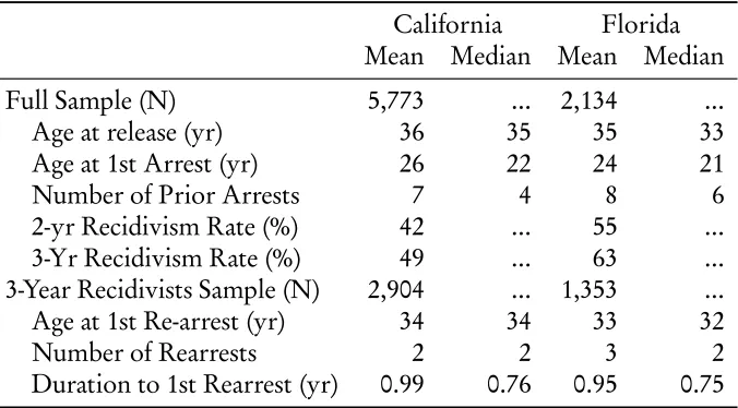
Table 1: Descriptive Statistics of the California and Florida Samples Used in the Analysis.
California Florida Mean Median Mean Median Full Sample (N) 5,773 ... 2,134 ... Age at release (yr) 36 35 35 33 Age at 1st Arrest (yr) 26 22 24 21 Number of Prior Arrests 7 4 8 6 2-yr Recidivism Rate (%) 42 ... 55 ... 3-Yr Recidivism Rate (%) 49 ... 63 ... 3-Year Recidivists Sample (N) 2,904 ... 1,353 ... Age at 1st Re-arrest (yr) 34 34 33 32
Number of Rearrests 2 2 3 2
Duration to 1st Rearrest (yr) 0.99 0.76 0.95 0.75
To make the estimation problem feasible (and realistic), data from only the state of California were used for estimating the model. The models, once es-timated, were validated using data from the state of Florida. These two states were selected from the 15 states included in the underlying data for two reasons. First, they were the largest states in this dataset (in terms of unweighted sample sizes). Second, the unweighted three-year recidivism rate (one of the chief crite-rion variables) was roughly 50% for the California sample but roughly 65% for the Florida sampla. This offers some insights into the out-of-sample predictive performance of the strategy on a validation sample somewhat more crimino-genic than the estimation one. Other than that, the two samples seems very similar (at least in terms of mean characteristics). Table 1 provides a prief sum-mary of the underlying data used for the two states. With the exception of the number of prior arrests before release, for which Florida seems a bit higher than California, the other predictors and manifestations seem very similar across the two states.
A serious limitation of the BJS Recidivism data is the lack of information on the amount of time that the offender may have served in prison in several incarceration episodes prior to the current one or post-release. Despite the avail-ability of adjudication information for each of the arrest cycles, the data do not contain clear information on the amount of time persons may have served in prison if they were incarcerated. This problem is not peculiar to this study alone. Accounting for street-time is a difficult matter in all retrospective or prospective longitudinal designs. The BJS data do, however, contain adjudica-tion outcomes of each of the cycles and the type of adjudicaadjudica-tion at an arrest event. This information is currently being used to derive additional relevant analogies for inclusion in the model as well as to include/exclude individuals from the risk set (i.e. to define f(t) appropriately). The work is ongoing and this measure is not included in the analysis reported here.
4.1. Model Estimates
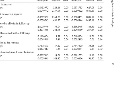
Table 2 provides estimates of the lagrange multipliers from the various analogous constraints imposed to derive the model. Using the negative inverted hessian, a standard error was computed and used to derive the Wald χ2 statistic. The
statistic indicates that almost all of the constraints have informational content. That is, they providestatistically significantinformation about the process under study. The single explnatory variables used in the modeling exercise—age at first arrest—seems to indicate that offenders who initiate their careers later in life, compared to those who start earlier, have parmanently lower hazards (negative coefficient under b); have an upward pressure on the evolution of the hazard with age (positive coefficient under a), but at a decreasing rate (negative coeffi-cient undera2); seem to have higher numbers of crimes accumulated by the end
/
Lear
ning
fr
om
Multiple
Analogies
16
cal Significance for Two-year and Three-year Follow-up Models.
2-Year Follow-up 3-Year Follow-up
Manifestations Lagrange Waldχ2 p- Lagrange Waldχ2 p
Predictors Multiplier Statistic value Multiplier Statistic value
a: Age at 1st rearrest
Intercept -0.0453972 328.16 0.00 -0.0571753 627.09 0.00
Age1st 0.0049772 2757.64 0.00 0.0059822 4846.11 0.00
a2: Age at 1st rearrest squared
Intercept -0.0009862 1164.06 0.00 -0.0008453 1009.52 0.00
Age1st -0.0000243 636.53 0.00 -0.0000344 1492.18 0.00
b: Rearrested at all within follow-up
Intercept -2.0000779 35.07 0.00 -4.1362998 144.41 0.00
Age1st -0.2274956 241.95 0.00 -0.2298919 237.84 0.00
c: Times Rearrested within followup
Intercept 0.1826634 4.31 0.04 0.7984504 118.71 0.00
Age1st 0.0068398 3.49 0.06 0.0002495 0.01 0.94
d: Duration to 1st rearrest
Intercept -0.7115693 17.22 0.00 0.7847820 34.15 0.00
Age1st 0.0177117 6.33 0.01 0.0020134 0.13 0.72
e: Times Arrested since Career Initiation
Intercept -0.0327985 14.08 0.00 -0.0281003 11.12 0.00
[image:17.612.141.651.157.482.2]the hazard path is an aggregation over all of these decompositions.
With few exceptions, the findings are identical across the two follow-up peri-ods. Notably, the effects of Age1st are statistically insignificant for the last three manifestations in the larger follow-up model.
4.2. Model Predictions
The multple analogy models estimated with the California sample were next used to make predictions. The chief criterion that models’ predictive efficacy is assessed on is whether they are able to predict failure at the end of the follow-up period (the binary outcome).In each case, the estimated hazard paths were integrated over the relevant domain and used to compute the probability of re-cidivism using the definition:
Pr(bn=1) =1−exp(− Z
T
ˆrn(t)d t)
Moreover, in each case, the mean recidivism rate of the criterion of interest was used to set the cut-off point to convert this predicted probability into a binary classification.
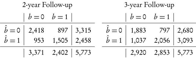
The first set of assessments are for in-sample predictions. That is, models are assessed on their ability to predict the outcomes using the data they were estimated with. These are typically the least challenging of prediction problems. Table 3 provides a cross-tabulation of the models’ predictions (bˆ) versus what was actually observed in the sample (b). The models perform fairly well—both within the 2-year ar the 3-year follow-up periods.
Table 3: Within Sample Predictive Efficacy of Multiple Analogy Models, California Sample.
2-year Follow-up 3-year Follow-up
b=0 b=1 b =0 b =1
ˆ
b=0 2,418 897 3,315 ˆb=0 1,883 797 2,680
ˆ
b=1 953 1,505 2,458 ˆb=1 1,037 2,056 3,093 3,371 2,402 5,773 2,920 2,853 5,773
The model in-sample predictive efficacy was somewhat lower at the 2-year window, although it was still good. Of those predicted to recidivate within the 2-year follow up period, nearly 61% did actually recidivate, and the remaining 38% were erroneous (false positives). However, of the 2-year recidivists, the models accurately identified 62% of them, but missed 38% of them.
Considering that the models used a minimal set of predictors—age at release, prior criminal history, and age at first arrest—and, of these, the first two were used to create new dependentvariables, the predictive accuracy of the models is quite surprising. It can be expected that as additional individual level attributes and, perhaps, demographic attributes are included in the models, they will per-form better yet.
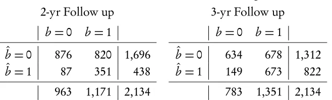
Although in-sample accuracy is interesting, the more challenging prediction problems are predicting out-of-sample and off-the-support. Table 4 presents a cross tabulation for assessing the out-of-sample predictive efficacy of the models by using the California model estimates (the Lagrange Multipliers) and gener-ating predictions—both at the 2-year and 3-year follow-up period—for the state of Florida. As one would expect, the models perform worse when estimating out-of-sample. Note the out-of-sample predictions being assessed here are for a different state. This is a different problem—a more realistic one—that taking a random subset of the estimation sample for validation purposes.
Table 4: Out-of-Sample Predictive Efficacy of Multiple Analogy Models, California Models Assessed on Florida Sample.
2-yr Follow up 3-yr Follow up
b=0 b=1 b =0 b =1
ˆ
b=0 876 820 1,696 ˆb=0 634 678 1,312
ˆ
b=1 87 351 438 ˆb=1 149 673 822 963 1,171 2,134 783 1,351 2,134
and 822 individual would fail within two and three years of release, respectively, whereas 1,171 nd 1,351 individuals actually recidivated within these respective follow-up periods. That is, the models predicted recidivism rates nearly half of what was actually observed. Despite that, the news was not all bad. At least at the three year window, despite very low aggregate predictions, the models were fairly good at finding the recidivists. Of those that actually recidivated within three years of release, the models correctly identified about half of them (49%). Similarly, of those few predicted to recidivate, nearly 81% were actually accurate with a false positive rate of only 19%. Therefore, despite predicting a recidi-vism rate only about half of what was actually observed, the models were fairly accurate in terms of those few that they did identify as recidivists.
The performance of the model was somewhat less encouraging at the two year follow-up period, though. Once again, the models only predicted a recidi-vism rate about half of the actual rate. However, as in the three year case, of those that the model identified as recidivists, nearly 80% were accurate, with a 20% false positive rate. However, at the two year window, the model missed a large portion of actual recidivists. Nearly 70% of those that did fail were not accurately identifed by the models. In some sense, then, the California mod-els were providing conservative predictions in the Florida sample. The modmod-els did not classify nearly enough sample members as recidivists. When they did, however, they were surprisingly accurate.
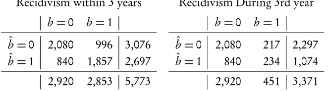
off-the-Table 5: Off-the-Support Predictive Efficacy of Multiple Analogy Models, California 2 year Follow up Models Assessed on 3 Year Recidivism.
Recidivism within 3 years Recidivism During 3rd year
b=0 b=1 b =0 b =1
ˆ
b=0 2,080 996 3,076 ˆb=0 2,080 217 2,297
ˆ
b=1 840 1,857 2,697 ˆb=1 840 234 1,074 2,920 2,853 5,773 2,920 451 3,371
support predictions. Here, models estimated on a 2-year support were used to make projections for a 3-year window. Table 5 provides cross-tabulation for assessing the predictive efficacy of the California 2-year models for projecting 3-year recidivism in California. The first cross-tabulation uses predictions of the
three-year recidivism rate were as the second cross-tabulation uses predictions of thethird-yearrecidivism rate.
The model projected considerably well when considering the three-year re-cidivism measure. The two year model projected a slightly lower overall 3-year recidivism rate (47%) than was observed in the sample (49%). Moreover, of the 2,697 individuals predicted to recidivate within three years of release, 68% actu-ally did. About 31% of these projections were erroneous. On the other hand, of the 2,852 individuals who did recidivate within three years of release, the mod-els correctly identified 65% of them. The modmod-els only missed about a third of them.
[image:21.612.141.473.177.269.2]1,074 individuals would recidivate within the third year of release where as only about 451 actually did. With this over-projections also came a high false positve rate. Of the 1,074 individuals predicted to recidivate during the third year, only about 22% actually did. The false positve rate was very high (nearly 81%). On the other hand, the model had a surprisingly decent hit rate. Of the 451 indi-viduals that did recidivate within the third year of release, the models correctly identified 52% of them.
5. CONCLUSION
The goal of this paper was to develop and apply a semi-parametric, information theoretic approach for utilizing knowledge in multiple analogies for studying and predicting criminal recidivism. It was expected that, despite relying on a minimal set of predictors, models consistent with several analogies simultane-ously should perform well. Although the relative performance of multiple anal-ogy models—both relative to other types of modeling strategies or to models using fewer/more analogies—is yet to be gauged, preliminary findings presented in this paper suggest that the strategy holds promise.
5.1. Discussion of Findings
about the recidivism process “significantly.”
The estimated models were next used to make predictions. Not surprisingly, the in-sample predictive performance of the models were very good. The false positive and false negative rates of the three year model were 34% and 30% re-spectively and those of the two year model were 38% and 29% repectively. Sim-ilarly, the hit rates—proportion of actual recidivists correctly identified—for the three and two year models were, respectively, 72% and 63%.
The estimated California models were also used to predict recidivism among the Florida sample. These out-of-sample predictions were less enocouraging. Despite having acceptible false positive and negative rates (respectively, 18% and 51% for the three year predictions and 20% and 48% for the two year predic-tions), the hit rate was usually low, particularly for the 2 year predictions (50% and 30% for the three and two year predictions, respectively). The models were conservative, though. They predicted very few recidivists but, among those pre-dicted, the error rate was very low.
Finally, the models were gauged on their ability to predict off-the-support. Here the findings were mixed. The two year models predicted failure within three years of release fairly well. However, they were not that accurate at pre-dicting failure within the third year of release. The two-year models predicted nearly 3 times as many third-year recidivists as there really were in the sample. An unacceptibly large proportion of these were false positives (78%). However, even these predictions had a decent hit rate. The predictions were able to accu-rately identify nearly half of those that actually did recidivate during the third year.
The analysis conducted here was very limited. However, the preliminary findings are encouraging and offer several insights.
Second, the out-of-sample predictions were fairly low. This findings is also not suprising, on hind sight. Table 1 shows that the sample of Florida was very similar to the sample in California, as least with respect to the attributes used. However, the failure rate in the Florida sample was considerably higher than that in the California sample. This suggests, perhaps, that the main differences between California and Florida samples was not the individual attributes of the offenders, but the punitiveness of the system or data definition or collecting pe-culiarities. Since the modeling strategy does not takes these differences into ac-count, it should be expected that model estimates from California would under-predict recidivism when used on the Florida sample. The systematic differences between states can be accounted for by appropriately defining the priors (in this analysis the ¯rn(t)). Such advances are currently being developed. However, it is encouraging that despite the overall underprediction of the phenomenon in Florida, the models were conservative (low false positive rates).
Third, the analysis did not take into account various cut-off criteria to make predictions. Judicious selections of an optimal cut-off point for each model may further improve the predictive performance of the models.
5.2. Ongoing and Future Research
The preliminary set of models developed in this paper were designed to gain some insights into the working of the approach and to gauge its predictive per-formance. Given the minimal set of predictors included, the models seem to perform surprisingly well. There are several aspects of the strategy that need further exploration.
Second, other relevant analogies need to be developed that can allow ana-lysts to incorporate knowledge about crime-type-specific recidivism manifesta-tions. For example, a hazard models of general recidivism could have two sub-components—one relating to violent and another to non-violent crimes. Each of these sub-components should yield nuanced insights into the process although the ultimate interest may be in predicting general recidivism. This work is cur-rently under way.
Third, the models, so far, have completely ignored the issues relating to re-incarceration. This needs to be addressed. Although the data source provides less than perfect informationn about this aspect of the model, analogies are cur-rently being developed that will allow the model to learn from such outcomes as whether or not the individual was reincarcerated within the follow-up period, how many times, and the duration to first reincarceration event in addition to outcomes relating to the binary, count, and duration manifestations of rearrest. Finally, a more elaborate assessment of the predictive efficacy of this mod-elling strategy needs to be undertaken. This includes comparing the multiple analogy models with other state-of-the-art survival models as well as using tools like the receiver operating characteristic curves to compare models across a range of cut-off points. This work is currently underway.
MATHEMATICAL APPENDIX
Since a key component of the procedure for learning from multiple analogies outlined in the narrative was the functional form of the information criterion (3), this appendix provides a brief derivation of this measure based on a minimal set of plausible assumptions.
properties for the function f to possess?
The first set of assumptions pertain to the range of values information can take. Keeping in mind that all quantities are indexed by t (i.e., we are talking about information at a particulart), let
f ≥ 0 ∀r, ¯r >0 (8a)
f = 0 ∀r=¯r (8b)
Here, (8a) states that information is a non-negative quantity for all values of the prior and posterior hazard rates and (8b) states that if the posterior is exactly the same as the prior, then no information has been acquired.
The second set of assumptions deal with how information changes as the absolute value of the posterior increases. Let
d f
d r > 0 ∀r >¯r (9a) d f
d r < 0 ∀r <¯r (9b) d f
d r = 0 ∀r =¯r (9c)
These assumptions simply state that the amount of information increases if the posterior moves further away from the prior—whether or not r is higher or lower than ¯r. For example, (9a) implies that if r >¯r then an increase in r adds to information since it takes the analyst further away from the prior. Similarly, (9b) implies that if r <¯r then an increase in r brings the analyst closer to the prior. (9c) implies that f is continuous in r.
hazard were low. This assumptions translates to d f d r
r=r1 >d f
d r
r=r2
∀r1<r2 (10a)
or, put another way, it translates to the second order differential equation
d2f
d r2 = κ0
r ∀r (10b)
whereκ0is the constant of proportionality that can be set to any arbitrary
con-stant without loss of generality. Since the ultimate goal is to derive a measure that will be optimized (maximized or minimized), a scaling constant will make no difference to the final solution of this optimization problem.
Given these assumptions, and setting the constant of proportionality to 1, we can start by integrating (10b) to get
d f d r =
Z
R 1
r d r =log(r) +κ1
where the constant of integration,κ1, can be solved using the initial condition
(9c) to getκ1=−log(¯r). This yields the result
d f d r =log
r
¯
r
which, it can be verified, satisfies each of the conditions (9a)–(9c). This solution can be further integrated to obtain
f =
Z
R log r
¯r d r =rlog r
¯r −r +κ2
where the constant of this integration,κ2, can be solved using the initial
condi-tion (8b) to getκ2=¯r.
conditional (on t) aspect of this measure, we can compute the net information acquired over the entire domainT as
I =
Z
T
I(t)d t =
Z
T
r(t)logr(t)
¯r(t)−r(t) +¯r(t)
d t (11)
Since the analyst modeling criminal recidivism has information only on a limited support of the domainT (e.g., the follow-up period) the measure in (3) appropriately restricts the computation in (11) to a limited support.
Note that (11) is a more general measure of information than the Kullback-Leibler directed divergence measure commonly used in Information Theory (Kullback 1959). To see this, note that if the prior and posteriors were in fact proper probabilities (integrating to 1) then the measure in (11) could be simpli-fied to
I =
Z
T
r(t)logr(t) ¯r(t)d t−
Z
T
r(t)d t+
Z
T
¯r(t)d t =
Z
T
r(t)logr(t) ¯r(t)d t
which is the Kullback-Leibler directed divergence measure between two proper densities. Moreover, with an uninformative or constant (over the domain) prior, the minimization of information amounts to the maximization of Entropy— precisely the procedure Edwin Jaynes initially proposed (Jaynes 1957a,b).
REFERENCES
Allison, P. (1982). Discrete-time methods for the analysis of event histories.
Sociological Methodology13:61–98.
Allison, P. (1984).Event history analysis: Regression for Longitudinal Data. New-bury Park: Sage.
Asadi, M., Ebrahimi, N., Hamedani, G. G., and Soofi, E. (2005). Minimum Dy-namic Discrimination information models. Journal of Applied Probability
42(3):643-660.
Bhati, A.S. (in press). Estimating the number of crimes averted by incapacita-tion: An Information Theoretic approach.”Journal of Quantitative Crim-inology.
Bhati, A.S. (2007). Studying the effects of incarceration on offending trajectories: An Information Theoretic approach. Washington, DC: The Urban Insti-tute.
Bhati, A.S., and Piquero, A.R. (under review). On the effect of incarceration on subsequent individual criminal offending: Deterrent, criminogenic, or null effects.
Beck, N. (1998). Modelling space and time: The event history approach. Pg. 191–213 in E. Scarbrough and E. Tanenbaum eds.Research strategies in the social sciences. New York, NY: Oxford University Press.
Box-Steffensmeier, J.M., and Jones, B.S. (2004). Event history modeling: A guide for social scientists. Cambridge, UK: Cambridge University Press.
Bureau of Justice Statistics. (2002). Recidivism of prisoners released in 1994, Code-book for dataset 3355. Downloaded from NACJD in April 2007.
Cameron, C., and Trivedi, P. (1998). The analysis of count data. New York, NY: Cambridge University Press.
Dean, C.B., and Balshaw, R. (1997). Efficiency lost by analyzing counts rather than event times in Poisson and overdispersed Poisson regression models.
Journal of the American Statistical Association92(440):1387–1398.
Diamond, S. (1959). Information and error: An introduction to statistics. New York, NY: Basic Books.
54:41-81.
Ebrahimi, N., Habibullah, M., and Soofi, E. (1992). Testing exponentiality based on Kullback-Leibler information. Journal of the Royal Statistical So-ciety B54(3):739-748.
Ebrahimi, N., and Kirmani, S. N. U. A. (1996). A characterization of the pro-portional hazard model through a measure of discrimination between two residual life distributions. Biometrika83(1):233-235.
Ebrahimi, N., and Soofi, E. (2003). Static and dynamic information for dura-tion analysis. Invited presentadura-tion given atA conference in honor of Arnold Zellner: Recent developments in the theory, method, and application of infor-mation and entropy econometrics. Washington, D.C. Accessed February, 2007 from
http://www.american.edu/cas/econ/faculty/golan/golan/Papers/8_20soofi.pdf
Ezell, M.E., Land, K.C., and Cohen, L.E. (2003). Modeling multiple failure time data: A survey of variance-corrected proportional hazard models with ap-plications to arrest data. Sociological Methodology33(1):111-167.
Glaser, D. (1955). The efficacy of alternate approaches to parole prediction.
American Sociological Review20:283–287.
Gottfredson, S.D., and Gottfredson, D.M. (1986). Accuracy of prediction mod-els. Pg. 212–290 in eds. Blumstein, Cohen, Roth, and Visher Crimi-nal careers and “career crimiCrimi-nals” volumes II. Washington, DC: National Academy Press.
Greene, W. (2000). Models with discrete dependent variables. Pg. 811–895 in
Econometric analysis(4th edition). Upper Saddle River, NJ: Prentice Hall.
Gull, S.F. (1989). Developments in maximum entropy data analysis. in Maxi-mum entropy and Bayesian statisticsed. Skilling, J. Boston, MA: Kulwer.
Heckman, J., and Singer, B. (1984a). Econometric duration analysis. Journal of Econometrics24:63–132.
Heckman, J., and Singer, B. (1984b). A method for minimizing the impact of dis-tributional assumptions in econometric models for duration data. Econo-metrica52:271–320.
Jaynes, E.T. (1957a). Information Theory and Statistical Mechanics. Physics Review106:620–630.
Jaynes, E.T. (1957b). Information Theory and Statistical Mechanics II. Physics Review108:171–190.
Jaynes, E.T. (1979). Where do we stand on maximum entropy? Pg. 15–118 in R.D. Levine and M. Tribus (eds.) The maximum entropy formalism. Cambridge, MA: MIT Press.
Jaynes, E.T. (1986). Bayesian methods: An introductory tutorial. Pg. 1–25 in J.H. Justice (ed.) Maximum entropy and Bayesian methods in applied statis-tics. Cambridge, UK: Cambridge University Press.
Jaynes, E.T. (1988). Discussion. American Statistician. 42:280–281.
Justice, J.H. ed. (1986). Maximum entropy and Bayesian methods in applied statis-tics. Cambridge, UK: Cambridge University Press.
Kalbfleisch, J.D., and Prentice, R.L. (1980). The statistical analysis of failure time data. New York: Wiley.
King, G. (1977). A solution to the ecological inference problem. Princeton, NJ: Princeton University Press.
King, G. (1989). Variance specification in event count models: From restric-tive assumptions to a generalized estimator. American Journal of Political Science33(3):762–784.
Kullback, S. (1959). Information theory and statistics. New York, NY: John Wiley.
Lancaster, T. (1990). The analysis of transition data. New York, NY: Cambridge University Press.
Langan, P.A., and Levin, D.J. (2002). Recidivism of prisoners released in 1994. Special report. Washington, DC: Bureau of Justice Statistics.
Levine, R.D. and Tribus, M. eds.The maximum entropy formalism. Cambridge, MA: MIT Press.
Lin, D.Y., Wei, L.J., and Ying, Z. (1998). Accelerated failure time models for counting processes. Biometrika85(3):605–618.
Lipton, D., Martinson, R., and Wilks, J. (1975). The effectiveness of correctional treatment: A survey of treatment valuation studies. New York, NY: Praeger Press.
Maltz, M.D. (1984).Recidivism. Orlando, FL: Academic Press, Inc.
Mathai, A.M. (1975). Basic concepts in Information Theory and statistics: Ax-iomatic foundations and applications. New York, NY: John Wiley.
Mayer, K.U. and Tuma, N.B. ed. (1990). Event history analysis in life course re-search. Madison, WI: The University of Wisconsin Press.
Michell, S.M., and Moore, W.H. (2002). Presidential uses of force during the Cold War: Aggregation, truncation, and temporal dynamics. American Journal of Political Science46(2):438–452.
Mittelhammer, R. C., Judge, G. G., and Miller, D. J. (2000). Econometric Foun-dations. Cambridge, UK: Cambridge University Press.
Ryu, H.K. (1993). Maximum entropy estimation of density and regression func-tions. Journal of Econometrics56:397–440.
Shannon, C.E. (1948). A mathematical theory of communication. Bell System Technical Journal27:379-423.
Sherman, L.W., Gottfredson, D., MacKenzie, D., Eck, J., Reuter, P., and Bush-way, S. (1997). Preventing crime: What works, what doesn’t, and what’s promising? A Report to the United States Congress. Washington, DC: National Institute of Justice. (http://www.ncjrs.gov/works )
Skilling, J. (1989). Maximum entropy and Bayesian methods. Dordrecht, the Netherlands: Kluwer.
Soofi, E.S. (1994). Capturing the intangible concept of information. Journal of the American Statistical Association89(428):1243–1254.
Soofi, E.S. (2000). Principal Information Theoretic approaches. Journal of the American Statistical Association95(452):1349–1353.
Soofi, E.S., Ebrahimi, N., and Habibullah, M. (1995). Information distinguisha-bility with application to analysis of failure data. Journal of the American Statistical Association90(430):657–668.
Winkelmann, R. (1995). Duration dependence and dispersion in count-data models. Journal of business & economic statistics13(4):467–474.
Yamaguchi, K. (1991). Event history analysis. Newbury Park, CA: Sage Publica-tions.