Construction and Application of Subdivision Surface Scheme Using Lagrange Interpolation Polynomial

(1)

http://dx.doi.org/10.4236/am.2014.53040

Construction and Application of Subdivision Surface

Scheme Using Lagrange Interpolation Polynomial

Faheem Khan*, Noreen Batool, Iram Mukhtar Department of Mathematics, University of Sargodha, Sargodha, Pakistan

Email: *_{[email protected]}_,_{[email protected]}_,_{[email protected]}

Received April 22, 2013; revised May 22, 2013; accepted May 30,2013

Copyright © 2014 Faheem Khan et al. This is an open access article distributed under the Creative Commons Attribution License, which permits unrestricted use, distribution, and reproduction in any medium, provided the original work is properly cited. In accor-dance of the Creative Commons Attribution License all Copyrights © 2014 are reserved for SCIRP and the owner of the intellectual property Faheem Khan et al. All Copyright © 2014 are guarded by law and by SCIRP as a guardian.

ABSTRACT

This paper offers a general formula for surface subdivision rules for quad meshes by using 2-D Lagrange inter-polating polynomial [1]. We also see that the result obtained is equivalent to the tensor product of (2N + 4)-point n-ary interpolating curve scheme for N ≥ 0 and n ≥ 2. The simple interpolatory subdivision scheme for quadrila-teral nets with arbitrary topology is presented by L. Kobbelt [2], which can be directly calculated from the pro-posed formula. Furthermore, some characteristics and applications of the propro-posed work are also discussed.

KEYWORDS

Subdivision Scheme; Interpolating Subdivision Scheme; Tensor Product Scheme; Auxiliary Points; Lagrange Interpolation Polynomial

1. Introduction

There are two general classes of subdivision schemes, namely, approximating and interpolating schemes. The limit curve of an approximating scheme usually does not pass through the control points of control polygon. As the level of refinement increases, the polygon usually shrinks towards the final limit curve. The interpolating schemes are more attractive than approximating schemes because of their interpolation property. All vertices in the control polygon are located on the limit curve of the interpolation scheme, which facilitates and simplifies the graphics algorithms and engineering designs.

Lian generalized the classical binary 4-point and 6-point interpolatory subdivision schemes to a-ary setting for any integer a ≥ 3. After that, the a-ary 3-point and 5-point interpolatory subdivision schemes for curve design for arbitrary odd integer a≥ 3 [3,4] were introduced. After that, Lian [5] investigated both the 2m-point, a-ary for any a ≥ 2 and (2m + 1)-point, a-ary for any odd a ≥ 3 interpolatory subdivision schemes for curve design. Ko [6] presented explicitly a new formula for the mask of (2N + 4)-point binary interpolating and approximating subdivision schemes with two parameters. The proposed work presents a new observation about the curve case given by Najma [7]. In this work, we avoid finding the mask of subdivision schemes separately, as a result, its approach is simple and avoids complex computation when deriving subdivision rules.

The rest of the paper is organized as follows. Section 2 gives some preliminaries results and a new relation for (2N + 4)-point n-ary interpolating curve scheme for closed and open polygon to access main result. Section 3 presents the construction for general formula of the surface case using Lagrange interpolating polynomial, and some characteristics are also discussed. In Section 4, we also give some numerical examples for the visual per-formance of the proposed work. This work also provides some special cases of the classical subdivision schemes.

*_{Corresponding author.}

(2)

2. Preliminary Results

Let  be the set of integers and a=

{

a ii ∈

}

a set of constants. The general form of univariaten-ary subdi-

vision scheme which maps a polygon k

{ }

ik i

f f

∈

=

 is defined by

1

0,1, 2, , 1, ,

k k

ni s nj s i j

j z

f ++ a + f− s n

∈

=

∑

=  − (2.1)

where the set a=

{

a ii ∈

}

of coefficients is called mask of the subdivision scheme. A necessary condition

for the uniform convergence of the subdivision scheme is

1, 0,1, 2, , 1,

nj s j z

a ₊ s n

∈

=

= −

∑

 (2.2)

Let Ω2N+1 be the space of all polynomials of degree ≤2N+1. Where, N is a non-negative integer. If

( )

{

}

N 1

N

Lµ x _µ

+

=− is fundamental Lagrange polynomial corresponding to the nodes

{ }

1

N N

µ

µ +

=− defined by

( )

1

,

N

j N j k

x j µ j L_µ x

+

=− ≠

− =

−

∏

(2.3)

for which

( )

, , , , 1

µ µ j

L j =δ − µ j= −N N+ and

( ) ( )

( )

1

2 1

,

N

N N

p L_µ x p x p

µ

+

+ =−

= ∈ Ω

∑

where, δ_{µ j}_, is the Kronecker delta, defined as

,

1,

0, µ j

j j

µ δ

µ

= ≠  = 

 (2.4)

Using all the above mentioned identities Ko [6] presented the general formula for the mask of

(

2N+4

)

-point binary interpolating symmetric subdivision schemes. After that Najma [7] generalized the result for

(

2N+4

)

-point n-ary interpolating symmetric subdivision scheme and gave the following formula for the mask of n-ary interpolating schemes.

(

)

(

)

( )

(

)

( )

(

)

, ,0 2

1 1 2 1 3

, ,

, , , , , ,

n j j

nj s n N s n N t

a v N j

a N j n s a N j a N j

δ ξ

ξ ξ ξ

+ + + + +

= −

− −



 ₌

 (2.5)

where

(

)

(

)

( )

(

1

)(

) (

)

1 , , , 2 1 ₁ 1 _! ₁ _!,

N

b N j N N

ni s N j n s

n s nj N j N j

ξ =− −

− + − +

+ =

− + − + +

∏

(

)

₍

( )

_{) (}

( )

(

_{) (}

)

₎

2

1 2 2 !

, ,

! 1 ! 1

j N

N N j

N j N j N j

ξ

+

− +

=

− + + − +

(

)

₍

( )

_{) (}

1

(

_{) (}

)

₎

3

1 2 2 !

, ,

! 1 ! 2

j N

N N j

N j N j N j

ξ

+ +

− +

=

− + + − +

and

( 1) ( 2)

n N s n N s

(3)

The free parameters a_{n N}₍ _{+ +}₁₎ _s can be explicitly defined as

( 1)

(

_{( )}

)(

(2 3)

_{( )}

)

(2

(

3)

₍

(

₎

)

2 2

! , 3

1 2 3

n N s N N

d n d n d Nn n

a

n N

+ + + +

− − +

− +

=  −

where d=n N

(

+ +1

)

s.

Here, n stands for n-ary subdivision scheme (i.e. n = 2(binary), 3(Ternary), 4(quaternary)

···

), N≥0, 1, , , 0,1, 2, , 1 and

j= − −N  N s=  n− t= −n s. Considering the symmetry of the scheme and construction of the mask formula described above,

(

2N+4

)

-point interpolating subdivision schemes are presented in the fol-lowing form

2 1

2 2

1

, where 0,1. N

k k

i l i l

l N

f _α a _αf α

+ +

+ − +

=− −

=

_∑

= (2.7)

Here, N≥0 with the symmetry condition is

( ) ( )

2N 1 2N 1

a₋ _{+ −}_α =a _{+ +}_α

Setting a₂₍_N₊₂₎=0 and a₂₍_N₊₂₎ =ν , the mask a2l−α of the schemes comes from the generalized formula

for the mask of

(

2N+4

)

-point interpolating schemes (2.5). Following the procedure of binary case, we have derived the following form of

(

2N+4

)

-point ternary interpolating subdivision schemes are presented in the following form

2 1

3 3

1

, where 0,1, 2. N

k k

i l i l

l N

f _α a _αf α

+ +

+ − +

=− −

=

∑

= (2.8)

Here, N≥0 and for the symmetry condition, a₋₃₍_N_{+ −}₁₎ _α =a₃₍_N_{+ +}₁₎_α

Setting a₃₍_N₊₂₎ =0 and a₃₍_N₊₁₎=v, the mask a3l−α is calculated from the same mask formula (2.5). In the

same way,

(

2N+4

)

-point quaternary interpolating subdivision scheme has the form 2

1

4 4

1

, where 0,1, 2, 3. N

k k

i l i l

l N

f _α a _αf α

+ +

+ − +

=− −

=

∑

= (2.9)

where, N≥0 and for the symmetry of the scheme, a₋₄₍_N_{+ −}₁₎ _α =a₄₍_N_{+ +}₁₎_α.

Setting a₄₍_N₊₂₎=0 and a₄₍_N₊₁₎ =v. Finally, from (2.7)-(2.9),

(

2N+4

)

-point n-ary interpolating schemes has the following form

2 1

1

, where 0,1, 2, , 1, N

k k

ni nl i l

l N

f _α a _αf α n

+ +

+ − +

=− −

=

∑

=  − (2.10)

With N≥0,n≥2, and for the following symmetry condition ( 1) ( 1) n N n N

a₋ _{+ −}_α =a _{+ +}_α (2.11) where a_{n N}₍ ₊₂₎ =0 and a_{n N}₍ ₊₁₎=v.

Construction of the Schemes for Open Polygon

When dealing with open initial polygon 0

{

0

}

, : 0, ,

i

f = f i=  N it is not possible to refine the first and last edges by rules (2.10) for interpolating subdivision schemes. However the extension of this strategy to deal with open polygon requires a well-define neighborhood of end points. Since the first and last edges can be treated analogously, it will be sufficient to derive the rules only for one side of the polygon. To this aim define the auxiliary point f−0i =2f00−fi0 as extrapolatory rule in the initial polygon

0

f . Then the nonrefined open polygon

(4)

(

2N+4

)

-point interpolating scheme using auxiliary points is defined as following

( )

(

)

1 2

1

0 1 1

1

2 ,

i b

k k k k

ni nl nl i nl i

l N l i

f _α a _αf a _αf a _αf

− − +

+

+ − − − + − +

=− − =−

=

_∑

− +

_∑

(2.12)

where α=0,1, 2,,

(

n−1

)

, N≥0,i=0,1,,N and n≥2, where, the weights satisfies the same condition (2.11).

Example: If an open polygon is refined by using the 6-point ternary interpolating subdivision scheme using (2.10), then two auxiliary points f−02 = f00− f20 and

0 0 0

1 2 0 1

f− = f −f has to be defined in the coarsest polygon

0

f . The first two edges 0 1

k k

f f and 1 2

k k

f f of the nonrefined polygon

{

fik:i=0,, 3kN

}

can be refined by the rules that can be calculated directly by (2.12). Substituting n=3,N =1 in (2.12),

( )

(

)

1 1

3 3 0 3 3

2 0

3

2 ,

i

k k k k

i l l i l l i l

l l

f _α a _αf a _αf a _αf

− − +

+ − − − + − +

=− =

− +

=

∑

where α=0,1, 2.i=0,1. Then, for i=0,

(

)

(

)

(

)

1

0 2 6 2 3 0 0 3 3 1 6 6 2 9 3,

k k k k k

f + = a₋ + a₋ +a f + a −a₋ f + a −a₋ f +a f

(

)

(

)

(

)

1 1 2

1

7 4 0 4 1 5 7 2 8 3

2 2 ,

k k k k k

f + = a₋ + a₋ +a₋ f + a −a₋ f + a −a₋ f +a f

(

)

(

)

(

)

2 2 1

1

8 5 0 5 1 4 8 2 7 3

2 2 .

k k k k k

f + = a₋ + a₋ +a₋ f + a −a₋ f + a −a₋ f +a f

For, i=1

(

)

(

)

1

6 3 0 6 1 3 2

3 2 0 6 3 9 4,

k k k k k k

f + = a₋ +a₋ f + a −a₋ f +a f +a f +a f

(

)

(

)

4 1 5 8 4

1

7 4 0 7 1 2 2 3 ,

2

k k k k k k

f + = a₋ +a₋ f + a₋ −a₋ f +a f +a f +a f

(

)

(

)

5 2 4 7 4

1

8 5 0 8 1 1 2 3 .

2

k k k k k k

f + = a₋ +a₋ f + a₋ −a₋ f +a f +a f +a f

3. Tensor Product of (2N + 4)-Point Interpolating Subdivision Scheme

Given a set of control points , , , , 2,

k N

i j

p ∈R i j∈Z N≥ where k is a non-negative integer indicates the subdivi-sion level. n-ary subdivisubdivi-sion surface is tensor product of n-ary subdivisubdivi-sion curve defined by

1

, , , ,

0 0

, , 0,1, , 1, m m

k k

ni nj r s i r j s r s

p +₊_α ₊_β a_α a_β p₊ ₊ α β n

= =

−

=

_∑∑

= _

(3.1)

where, aα,r satisfies

, 0

0,1 , 1

, , .

1

m

j j

aα α n

=

= −

∑

 (3.2)

Given initial values 0

, , , , , ,

N i j

p ∈R i j∈Z i j∈ then in the limit k→ ∞, the process (3.1) defines an infinite set of points in RN. The sequence of values

{ }

,

k i j

p is related, in a natural way, with a diadic mesh points , ,

k k

i j

n n

 

 

  i j, ∈Z. The process then defines a scheme whereby

1 ,

k ni nj

p +₊_α ₊_β replaces the value pi+αn j, +βn at the

mesh point ,

k k

i n j n

n n

α β

+ +

 

 

  for α β, ∈

{ }

0,n , while the values

1 ,

k ni nj

p +₊_α ₊_β are inserted at the new mesh points ni_k ₁ ,nj_k ₁

n n

α β

+ +

 

 

  for α β, =0,1,,n−1 (where α and β are not zero at the same time). Labeling of old

(5)

1, k i j p₊ , k i j p , 1 k i j

p + 1,1

k i j

p+ +

1 2 ,2 1

k i j

p+ + 1

2 ,2 2

k i j

p+ +

1 2 1,2 2

k

i j

p++ + 212,2 2

k

i j

p+₊ ₊

1 2 2,2 1

k

i j

p+₊ ₊

1 2 2,2

k

i j

p++ 1

2 1,2

k

i j

p++ 1 2 ,2 k i j p+ 1 2 ,2 1

k i j

p+ +

1 3 1,3 3

k

i j

p++ +

1, k i j p+ , k i j p ,1 k i j

p + 1, 1

k i j

p+ + 1 3 2,3 3

k

i j

p++ + 1 33,3 3

k

i j

p++ + 1

3 ,3 3

k i j

p+ +

1 3 3,3 2

k

i j

p++ +

1 3 3,3 1

k

i j

p++ + 1

3 ,3 2

k i j

p+ +

1 3 ,3 1

k i j

p+ +

1 3 ,3

k i j

p+ 3 1,31

k

i j

p++ 1 3 2,3

k

i j

p++ 1 33,3

k

i j

p++

1 4 2,4 4

k

i j

p++ + 414,4 4

k

i j

p+₊ ₊

1 4 4,4 2

k

i j

p+₊ ₊

1 4 ,4 2

k i j

p+ + 1 4 ,4 4

k i j

p+ +

1 4 ,4

k i j

p+ 1

4 2,4

k

i j

p++

1, k i j p₊ , k i j p , 1 k i j

p ₊ k_1, ₁

i j

p_{+ +}

1 4 4,4

k

i j

p++

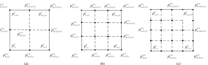
[image:5.595.96.536.82.221.2]

(a) (b) (c)

Figure 1. Solid lines show one face of coarse polygons whereas dotted lines are refined polygons. (a)-(c) can be ob-tained by subdividing one face into four, nine and sixteen new faces by using (3.1) for n = 2,3,4 respectively.

Construction

Let be the set of integers and the space of all polynomials of degrees ≤2γ +1 and ≤2σ+1 is denoted by 2γ+1

Ω and Ω2σ +1 respectively. If

{

( )

}

1

µ _µ

L x γ

γ

+

=− are fundamental Lagrange interpolating polynomials corres-

ponding to the nodes

{ }

µ γ_µ+₌₋1_γ and

{ }

υ σ_{υ σ}₌₋+1 . The Lagrange interpolation polynomial for tensor product case is defined as [1],

(

,

)

1 1 µ,?

(

,

) (

,

)

,

µ

p x y L x y p

γ σ

υ

γ υ σ

µ ν

+ + =− =−

=

_{∑ ∑}

where

(

)

1 1

,?

, ,

µ

i i j j

x i x j

L x y

i j

γ υ

υ

γ µ σ υµ υ

+ +

=− ≠ =− ≠

− −

= ×

− −

∏ ∏

(3.3)

, , 1, , , 1.

µ= −γ  γ+ υ= −σ σ+

,

µ i

δ and δυ_,_j are Kroneker delta symbols defined as,

, 1, 0, µ i i i µ δ µ = ≠  =   and , 1, 0, i i i ν ν δ ν = = ≠   

Here, some important results for the formulation of required form of tensor product scheme can be verified using (2.3). That is for each µ= − −γ 1,,γ and υ= −σ−1,,σ (Using the result [1]),

(

1

)

₍

( ) (

_{) (}

1 2

_{) (}

2 !

)

₎

,

! 1 ! 1

i

L

i i i

γ

γ γ

γ γ γ

+ − − + − − + + − + = −

(

)

₍

( ) (

_{) (}

1 2

_{) (}

2 !

)

₎

1 ,

! 1 ! 1

j

L

j j j

σ _σ

σ

σ σ σ

+ − − + − − + + − + = −

(

2

)

₍

( )

_{) (}

1 1

(

2

_{) (}

2 !

)

₎

,

! 1 ! 2

i

L

i i i

γ _γ

γ

γ γ γ

(6)

(

2

)

₍

( )

_{) (}

1 1

(

2

_{) (}

2 !

)

₎

,

! 1 ! 2

j

L

j j j

σ

σ σ

σ σ σ

+ + − − + + − + + + + = ( )

(

)

( ) ( )

(

)(

) (

)

1 1 1

2 1 1

1

2 2 1

2 1

2 ₂ ₁ ₂ ₂ ₁ _! _{1 !}

b

i i

nb s

s L

n _n _ni _s _i _i

γ γ

γ γ _γ _γ

=− + − + − + − + + + − + + −  _{ =}     + +

∏

( )

(

)

( ) ( )

(

)(

) (

)

1

2 1 1

2 2

2

2 2 1

2 1

,

2 2 1 2 2 1 ! 1 !

b

j j

mb s

s L

m m mj s j j

σ σ σ σ σ σ =− + − + − + −  + + + − + + − + =    +  

∏

(

)

( )

(

)(

) (

)

1 1 1 2 1 1 1 ,

1 ! 1 !

b

i i

nb s L

ni s i i

s

n n

γ γ γ

γ _γ _γ

=− − −   =  ₊ − + −   + − + − + +

∏

(

)

( )

1

(

1

)(

) (

)

2 1

2 2

2

.

1 ! 1 !

b j j mb s L mj s s j

m _m _j

σ σ σ σ σ σ =− − −   = _{ } + − + − + − + − + +

∏

The mask of a subdivision scheme shows the contribution of a single original vertex to each new, subdivided vertex. To find the mask of a scheme, we need to find all ways to get from the origin to each point in the grid. For the tensor product scheme, this is simply the tensor product of the univariate case.

Lemma 3.1. [8] Given initial control polygon 0

. ,

i j i j

p = p , i j, ∈Z，let the values . ,

k i j

p k≥1 be defined recursively by subdivision process (3.1) together with (3.2) then the scheme derived by tensor product naturally get four-sided support region.

It can be loosely say that the support is the tensor product of the supports of the two regions, just as one can loosely say that Doo-Sabin is the generalization of the tensor product of two Chaikin constructions.

Lemma 3.2. [9] Given initial control polygon pi j0, = pi j, , i j, ∈Z, let the values , , 1

k i j

p k≥ be defined re- cursively by subdivision process (3.1) together with (3.2), then if a scheme is derived from a tensor product, then the level of continuity can be determined between pieces by reference to the underlying basis functions, i.e. all the tensor product schemes have the same continuity as their counterparts.

The general formula which generates the mask

{ }

2 3 2 3

i i

a _{=− −}γ+_γ and

{ }

2 3 2 3

j _j

a σ₌₋+_σ₋ of n-ary approximating schemes presented by [7] is

( )

(

)

₍ ₎

( )

₍ ₎

( )

1 1 1

,0 2

1 1 1 2 1 3

,

, , , , , ,

ni i

ni s n s n t

a v j

a i n s a _γ i a _γ i

δ ξ γ

ξ γ ξ γ ξ γ

+ + + + + =  − = − −  

 (3.4)

and

(

)

(

)

₍ ₎

( )

₍ ₎

(

)

2 2 2

,0 2

1 2 1 2 1 3

,

, , , , , ,

mj j

mj s n s n t

a v j

a j n s a _σ j a _σ j

δ η σ

η σ η η η σ

+ + + + +

= −

= − −

 

 (3.5)

where

(

)

( )

(

)

( ) ( )

(

)(

) (

)

1 1

1 1 2 1 1

1

, , , ,

1 ! 1 !

b i

nb s i n s

n ni s i i

γ γ γ γ ξ γ γ γ =− + + − + − + = − + − + +

∏

(

)

( )

(

)

( )

(

)(

) (

)

2 1

1 2 2 1 1

2

, , , ,

1 ! 1 !

b j

mb s j m s

m mj s j j

σ σ σ σ η σ σ σ =− + + − + − + = − + − + +

∏

( )

₍

( ) (

_{) (}

)

₎

2

1 2 2 !

, ,

! 1 ! 1

i

i i i

γ _γ

ξ γ

γ γ γ

+

− +

(7)

(

)

₍

( ) (

_{) (}

)

₎

2

1 2 2 !

, ,

! 1 ! 1

j

j j j

σ

σ η σ

σ σ σ

+

− +

− + + − + =

( )

₍

( )

_{) (}

1

(

_{) (}

)

₎

3

1 2 2 !

,

! 1 ! 2

i

i i i

γ _γ

ξ γ

γ γ γ

+ +

− +

− + + + + =

(

)

₍

( )

_{) (}

1

(

_{) (}

)

₎

3

1 2 2 !

, .

! 1 ! 2

j

j j j

σ

σ η σ

σ σ σ

+ +

− +

− + + + + =

Here, n, m stands for n-ary, m-ary subdivision schemes respectively (i.e n, m = 2(binary), 3(ternary), 4(quaternary)

···

), γ σ, ≥0 i= − −γ 1,, ,γ j= − −σ 1,, ,σ s₁=1, 2,,n−1, s2 =1, 2,,m−1,t1= −n s1,

and t2= −m s2

The free parameter ₍ ₎ 1 1

n s

a _γ_{+ +} and ₍ ₎ 2 1

m s

a _σ_{+ +} are defined as

( 1) 1

(

_{( )}

)(

2 3

_{( )}

)

2

(

3

₍

(

₎

)

2 2 3

,

1 2 3 !

n s

d n d n d n n

a

n

γ γ γ

γ γ

+ + + +

− −

= − +

− +



(3.6)

where d=n

(

γ+ +1

)

s1 and

( 1) 2

(

_{( )}

)(

2 3

_{( )}

)

2

(

3

₍

(

₎

)

2 2 3

,

1 2 2 3 !

m s

e m e m e m m

a

m

σ σ σ

σ σ

+ + + +

− −

= − +

− +



(3.7)

where e=m

(

σ+ +1

)

s2.

As each mask a_{i j}_, of the refinement rule satisfies a_{i j}_, =b b_i _j, where b b_i, _j are the mask of univariate sub-division schemes, then

(ni s mj s1, 2) ni s1 mj s2

a ₊ ₊ =a ₊ a ₊ .

The tensor product of

(

2N+4

)

-point interpolating subdivision scheme is presented as,

( 1 2 ) 1 2

1 2

2 2

1

, , ,

1 1

,

k k

ni mj nl ml i l j l

l l

f a f

γ σ

α β σ β

γ σ

+ +

+

+ + − − + +

=− − =− −

=

∑ ∑

(3.8)

where, α=0,1, 2,,

(

n−1

)

, β =0,1, 2,,

(

m−1

)

, γ σ, ≥0, and n m, ≥2 and symmetry conditions are, ( ) ( )

( ) ( )

1 1

1 1 .

n n

m m

a a

γ α γ α

σ β σ β

− + − + +

= = 



 (3.9)

Taking an₍γ+2₎ =am₍σ=2₎ =0, and the constants anl1− −1αand aml2− −1 β could be evaluated by using the results (3.4) and (3.5).

Example: Consider the tensor product of the 4-point DD interpolating subdivision scheme, while DD scheme can be calculated using the result (2.5) mentioned in Section 2. The Laurent polynomial of the scheme is given as

( )

1

(

3 1 1 3

)

9 1 9 1 .

16

a z = −z− + z− + + z − z

This implies

( )

(

3 1 3

)

1 1 1 1 1

1

9 1 9 ,

16

a z = −z− + z− + + z −z

( )

(

3 1 3

)

2 2 2 2 2

1

9 1 9 .

16

a z = −z− + z− + + z −z

Since, a

(

z1,z2

)

=a

( ) ( )

z a z1 2 then, we can obtain the Laurent polynomial of the 4-point tensor product

(8)

(

)

(

)

(

1

2 ,2 ,

1

2 1,2 1, , 1, 2,

1

2 ,2 1 , 1 , , 1 , 2

1

2 1,2 1 1, 1 , 1 1, 1 2, 1

1, , 1,

9 9 ,

9 9 1

9 9

9 81 81 9

,

1 16

1

, 16

1 256

k k

i j i j

k k k k k

i j i j i j i j i j

k k k k k

i j i j i j i j i j

k k k k k

i j i j i j i j i j

k k k

i j i j i j

f f

f f f f f

f f f f

+

+ − + +

+

+ − + +

+

+ + − − − + − + −

− +

− + + −

− − +

− +

=

+ −

=

)

2, 1, 1

, 1 1, 1 2, 1 1, 2

, 2 1, 2 2, 2

9

81 81 9

9 9

k k

i j i j

k k k k

i j i j i j i j

k k k

i j i j i j

f

f f f f

f f f

+ − +

+ + + + + − +

+ + + + +

         

 −



 + + − +



 − − +

 

(3.10)

Using the result obtained above for the tensor product of interpolatory scheme (3.8), tensor product of 4-point DD scheme can be calculated directly. Since the DD scheme has 1

C continuity, then by lemma (3.2) its tensor product has the same continuity. Substituting n=m=2 in (3.8) and (3.9), α β, =0,1 and γ σ= =0, the symmetry conditions becomes

2 2

,

a a

α α

β β

− − +

= 

 ₌

 (3.11)

then formula (3.8) attains the form,

( 1 2 ) 1 2 1 2

2 2 1

2 ,2 2 ,2 ,

1 1

,

k k

i j l l i l j l

l l

f +₊_α ₊_β a ₋_σ ₋_β f₊ ₊

=− =−

=

∑ ∑

(3.12)

As each mask ai j, of the refinement rule satisfies ai j, =b bi j, then

(2l1 ,2l2 ) 2l1 2l2 a ₋_σ ₋_β =a ₋_αa ₋_β

As n=m=2 so a4=0 for both n and m, when υ υ1= 2=0, 1 2

1 16

ω =ω = − , b1=b2=0 and s s1, 2=1 is

substituted in (3.8) and (3.9) our requirement is fulfilled, that is the rules (3.10) are obtained.

Example: A simple interpolatory subdivision scheme for quadrilateral nets with arbitrary topology is pre-sented by L. Kobbelt [2] which generates C1 surfaces in the limit. In the first step they present the refinement rules derived by the modification of the well-known Dyn et al. [10] 4-point interpolatory subdivision scheme for curve design. The natural way to define refinement operators for quadrilateral nets is therefore to modify a ten-sor product scheme such that special rules for the vicinity of non regular vertices are found.

The modified form of Dyn scheme can be evaluated by setting the value of n = 2, N = 𝜐𝜐 = 0, a4=0 and

3 16

a = −ω (where 0< <ω 2

(

5 1−

)

) in (2.10) and (2.11), the following refinement rules are obtained

(

)

(

)

1 2

1

2 1 1 1 2

8

. 16

,

16

k k

i i

k k k k k

i i i i i

f f

f ω f f ω f f

+

+ + − +

= +

= + − +

  

 (3.13)

They used the simple tensor product as the basis for the modification of refinement rules of irregular quadri-lateral nets. Since it is interpolating scheme, so 2 ,21 ,

k k

i j i j

f + = f and the edge points 2 11,2

k i j

f ₊+ and 2 ,21 1

k i j

f + ₊ are given as,

(

)

(

)

(

)

(

)

1

2 1,2 , 1, 1, 2,

1

2 ,2 1 , , 1 , 1 , 2

8

,

16 16

8

.

16 16

k k k k k

i j i j i j i j i j

k k k k k

i j i j i j i j i j

f f f f f

ω ω

+

+ + − +

+

+ + − +

+

= + − +

+ = 



+ −



+ 

(9)

Finally, the face point 2 1,21 1

k i j

f +₊ ₊ is,

(

)

(

)

(

)

(

)

(

)

(

)

(

)

(

)

(

)

(

)

(

)

(

)

1 2

2 1,2 1, 1 , 1 1, 1

2 2

2

2, 1 1, , 1,

2

2, 1, 1 , 1

2 2

1, 1 2, 1 1, 2

, 2

1

8 8

256

8 8 8

8 8

k k k k

i j i j i j i j

k k k k

i j i j i j i j

k k k

i j i j i j

k k k

i j i j i j

k

i j i

f f f f

f f f

f f

ω ω ω ω ω

ω ω ω ω

+

+ − − − + −

+ − − +

+ − + +

+ + + + − +

+ +

= − + − +

+ − + + + + +

− + − +



+

+ + − +

− −



+

+ +



+

)

2

1, 2 2, 2

k k

j+ +ω fi+ j+

(3.15)

Instead of taking the tensor product the above rules can be directly obtained by substituting n=m=2 in (3.8) and (3.9), then α β= =0,1 and γ σ, =0, the symmetry conditions are then written as,

2 2

,

a a

α α

β β

− − +

= 

 ₌

 (3.16)

then the formula (3.8) acquires the form,

( 1 2 ) 1 2 1 2

2 2 1

2 ,2 2 ,2 ,

1 1

,

k k

i j l l i l j l

l l

f +₊_α ₊_β a ₋_σ ₋_β f₊ ₊

=− =−

=

_{∑ ∑}

(3.17)

At each mask ai j, of the refinement rule satisfies ai j, =b bi j, then (2l1 ,2l2 ) 2l1 2l2

a ₋_σ ₋_β =a ₋_αa ₋_β

Using the result (3.4) and (3.5) the constants a2l₁−α and a2l₂−β are evaluated by substituting υ υ1= 2 =0,

3 16

a = −ω , γ σ= =0, s s₁, ₂=1 and a4=0 for both n and m. After substituting the weights in (3.17) we

get the same rules (3.14) and (3.15).

Example: Using the results for the interpolating curve subdivision schemes (2.10) the 4-point interpolatory scheme [3] is obtained. Further here the tensor product of the scheme is evaluated by using the result (3.8). Put n= =m 3,b1=b2=0 in (3.8),

( 1 2 ) 1 2 1 2

2 2 1

3 ,3 3 ,3 ,

1 1

,

k k

i j l l i l j l

l l

f ++α +β a −σ −β f+ + =− =−

=

∑ ∑

(3.18)

Also, from (3.9)

2 2

,

a a

α α

β β

− − +

= 

 ₌



Taking α β= =0,1, 2, υ υ1= 2=a3=0,ω ω1 = 2 =a5 = −5 81, µ1=µ2=a4= −4 81. Also for

interpola-tory scheme a_n₍_γ₊₂₎ =a_m₍_σ₊₂₎=0, as n=m=3gives a6=0 for both n and m.

After calculating the mask from (3.4) and (3.5) and substituting all the results in equation (3.18) following 4-point ternary interpolating tensor product scheme is obtained

(

)

(

)

(

)

1

3 ,3 ,

1

3 1,3 1,

1

3 2,3 1,

1

3 ,3 1 ,

, 1, 2,

, , 1 , 2

1

, 1

60 30 4

5 ,

4 ,

81 1

30 60 5

81 1

60 30 4

81 5 ,

k k

i j i j

k k

i j i j

k k

i j i

k k k

i j i j i j

k k k

i j i j i j

k k k

i j i

j

k k

i j i j j i j

f f

f f f

f f

f

f f

f

f f

f

+

+ −

+

+ −

+ +

+

−

+ +

+

+ +

+ + =

= −

=

+

−

+ −

(10)

(

, 1 1, 2,

1, , 1, 2,

1, 1 , 1 1, 1 2, 1

1, 2 , 2 1,

1

3 1,3 1 1,

2 1

2

1

240 120 16

6561

150 1800 900 120

300 3600 1800 240

25 300 15

20

0 20

k k k

i j i j i j

k k k k

i j i j i j i j

k k k k

i j i j

k k

i j i j

k k k

i j i j i j i

i j i j f f f

f f f f

f f

f

f f

f − + +

− + +

+

+ + − −

− + + + + + +

− + + + + +

− − +

− + + −

=

− + + −

+ − − + k _,j+₂

)

,

(

, 1 1, 1 2, 1

1, , 1, 2,

1, 1 , 1 1, 1 2, 1

1, 2 , 2

1

3 2,3 1

1 2

1,

, 1

1

150 300 25

6561

240 1800 3600 300

120 900 1800 150

16 120 4

0

0 2

2 2

k k k k k

i j i j i j

k k k k

i j i j i j i j

k k k k

i j i j i j i j

k k k

i j i j i

j i

j

i j f f f

f f f f

f

f f

− + − + −

− +

+ +

+

− + + + + + +

− + +

+ − −

+ +

− − +

− + + −

+ − − +

=

)

2, 2

0fik+ j+ ,

(

)

1

3 ,3 2 , 1 , , 1 , 2

1

30 60

4 5

81 ,

k k k

i j i j i

i j j

k k

i j f f

f + + = − f − + + + − f +

(

, 1 1, 1 2, 1

1, , 1, 2,

1, 1 , 1 1, 1

1

2, 1

1, 2 , 2 1

3 1,3 2 1, 1

, 2

1

240 120 16

6561

150 1800 900 120

300 3600 1800 240

25 30

2

50 2

0

0 1 0

k k k

i j i j i j

k k k k

i j i j i j i j

k k k k

i j i j

k k

i j i j

k k k

i j i j i j

f f f

f f f f

f

f f

− + − + −

− + +

− + + + + + +

+

+ +

− + + + +

− − − − +

− + + −

− + +

− −

=

−

+ + 2, 2

)

,

k

i j

f+ +

[image:10.595.115.512.57.541.2]

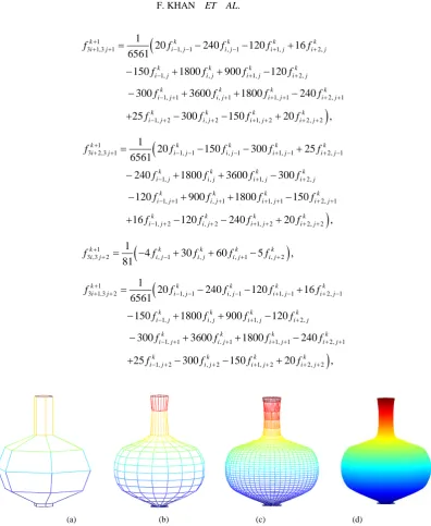
(a) (b) (c) (d)

Figure 2. Performance of tensor product of 4-point ternary interpolating scheme: (a), (b), (c) and (d) show the initial polygon, 1st, 2nd subdivision levels and limit surface respectively. (a) Initial polygon; (b) 1st level; (c) 2nd level; (d) Lim-it surface.

(a) (b) (c) (d)

[image:10.595.118.511.593.700.2]

(11)

Lim-it surface.

(

, 1 1, 1 2, 1

1, , 1, 2,

1, 1 , 1 1, 1

1

2, 1

1, 2 , 2 1

3 2,3 2 1, 1

, 2

1

120 240 20

6561

120 900 1800 150

240 1800 3600 300

20 15

1

00 2

6

0 3 5

k k k

i j i j i j

k k k k

i j i j i j i j

k k k k

i j i j

k k

i j i j

k k k

i j i j i j

f f f

f f f f

f f

f

− + − + −

− + +

− + + + + + +

+

+ +

− + + + +

− − − − +

− + + −

− + +

− −

=

− + + fik+_2,j+₂

)

,

(3.19)

4. Numerical Examples

Here, the performances of some of the schemes which are deduced from the proposed formula are shown. Fig-ure 2 shows the tensor product of 4-point ternary interpolating scheme (3.19), and Figure 3gives the perfor-mance of the proposed 4-point binary scheme (3.10).

REFERENCES

[1] G. Dahlquist and A. Bjork, “Numerical Methods in Scientific Computing,” SIAM, Vol. 1, 2008. http://dx.doi.org/10.1137/1.9780898717785

[2] L. Kobbelt, “Interpolatory Subdivision on Open Quadrilateral Nets with Arbitrary Topology,” Computer Graphics Forum, Vol. 15, No. 3, 1996, pp. 409-420.http://dx.doi.org/10.1111/1467-8659.1530409

[3] J. A. Lian, “On A-Ary Subdivision for Curve Design: 4-Point and 6-Point Inerpolatory Schemes,” Application and Applied Mathematics: International Journal, Vol. 3, No. 1, 2008, pp. 18-29.

[4] J. A. Lian, “On A-Ary Subdivision for Curve Design. II. $3$-Point and $5$-Point Interpolatory Schemes,” Applications and Applied Mathematics: International Journal, Vol. 3, No. 2, 2008, pp. 176-187.

[5] J. A. Lian, “On A-Ary Subdivision for Curve Design. III. 2m-Point and (2m+1)-Point Interpolatory Schemes,” Applications and Applied Mathematics: International Journal, Vol. 4, No. 2, 2009, pp. 434-444.

[6] K. P. Ko, “A Study on Subdivision Scheme-Draft,” Dongseo University Busan South Korea, 2007. http://kowon.dongseo.ac.kr/$\sim$kpko/publication/2004book.pdf

[7] G. Mustafa and A. R. Najma, “The Mask of (2b+4)-Point n-Ary Subdivision Scheme,” Computing, Vol. 90, No. 1-2, 2010, pp. 1-14.

[8] M. Sabin, “Eigenanalysis and Artifacts of Subdivision Curves and Surfaces,” In: A. Iske, E. Quak and M. S. Floater, Eds., Tu-torials on Multiresolution in Geometric Modelling, Chapter 4, Springer,Berlin, 2002, pp. 51-68.

[9] N. A. Dodgson, U. H. Augsdorfer, T. J. Cashman and M. A. Sabin, “Deriving Box-Spline Subdivision Schemes,” Sprin-ger-Verlag, Berlin, 2009, pp. 106-123.