A Regularized Newton Method with Correction for Unconstrained Convex Optimization

(1)

http://dx.doi.org/10.4236/ojop.2016.51006

How to cite this paper: Li, L.M., Qin, M. and Wang, H. (2016) A Regularized Newton Method with Correction for Uncon-strained Convex Optimization. Open Journal of Optimization, 5, 44-52. http://dx.doi.org/10.4236/ojop.2016.51006

A Regularized Newton Method with

Correction for Unconstrained

Convex Optimization

Liming Li, Mei Qin

*

, Heng Wang

College of Science, University of Shanghai for Science and Technology, Shanghai, China

This work is licensed under the Creative Commons Attribution International License (CC BY). http://creativecommons.org/licenses/by/4.0/

Abstract

In this paper, we present a regularized Newton method (M-RNM) with correction for minimizing a convex function whose Hessian matrices may be singular. At every iteration, not only a RNM step is computed but also two correction steps are computed. We show that if the objective function is LC2_{, then the method posses globally convergent. Numerical results show that the new algorithm}

performs very well.

Keywords

Regularied Newton Method, Correction Technique, Trust Region Technique, Unconstrained Convex Optimization

1. Introduction

We consider the unconstrained optimization problem [1]-[3]

( )

min ,

n

x R f x

∈

(1.1)

where f R: n→R is twice continuously differentiable, whose gradient ∇f x

( )

and Hessian ∇2f x

( )

are denoted by g x

( )

and H x

( )

respectively. Throughout this paper, we assume that the solution set of (1.1) is nonempty and denoted by X, and in all cases ⋅ refers to the 2-norm.

It is well known that f x

( )

is convex if and only if H x

( )

is symmetric positive semidefinite for all

n

x∈R . Moreover, if f x

( )

is convex, then x∈X if and only if x is a solution of the system of nonlinear

(2)

equations

( )

0.

g x =

(1.2) Hence, we could get the minimizer of f x

( )

by solving (1.2) [4]-[8]. The Newton method is one of efficient solution methods. At every iteration, it computes the trial step

1 , N

k k k

d = −H g− (1.3) where g_k =g x

( )

_k and H_k =H x

( )

_k . As we know, if H_k is Lipschitz continuous and nonsingular at the so-lution, then the Newton method has quadratic convergence. However, this method has an obvious disadvantage when the H_k is singular or near singular. In this case, we may compute the Moore-Penrose step [7]

MP

k k k

d = −H g+ . But the computation of the singular value decomposition to obtain H_k+ is sometimes prohibi-tive. Hence, computing a direction that is close to d_kMP may be a good idea.

To overcome the difficulty caused by the possible singularity of H_k, [9] proposed a regularized Newton method, where the trial step is the solution of the linear equations

(

Hk+

λ

kI d

)

= −gk, (1.4)

where I is the identity matrix. µ_k is a positive parameter which is updated from iteration to iteration.

Now we need to consider another question, “how to choose the regularized parameter µ_k?” Yamashita and Fukushima [10] chose λ_k = g_k 2 and showed that the regularized Newton method has quadratic convergence under the local error bound condition which is weaker than nonsingularity. Fan and Yuan [11] took λ_k = g_k δ with

δ

∈

[ ]

1, 2 and showed that the Levenberg-Marqulardt method preserves the quadratic convergence. Nu-merial results ([12][13]) show that the choice of

λ

_k = F_k performs more stable and preferable.

Inspired by the regularized Newton method [13] with correction for nonlinear equations, we propose a mod-ified regularized Newton method in this paper. At every iteration, the modmod-ified regularized Newton method first solves the linear equations

(

Hk+

λ

kI d

)

= −gk with

λ

k =

µ

k gk (1.5)

to obtain the Newton step d_k, where µ_k is updated from iteration to iteration, and solves the linear equations

(

Hk+

λ

kI d

)

= − +gk

λ

kdk (1.6)

to obtain the approximate Newton step s_k. It is easy to see

 

₍

₎

1

, .

k k k k k k k k

s =d +d d =λ H +λ I − d

(1.7) Then it solves the linear equations

(

Hk+

λ

kI s

)

= −g y

( )

k with yk =xk+sk (1.8)

to obtain the approximate Newton step s_k.

The aim of this paper is to study the convergence properties of the above modified regularized Newton me-thod and do a numerical experiment to test its efficiency.

The paper is organized as follows. In Section 2, we present a new regularized Newton algorithm with correc-tion by trust region technique, and then prove the global convergence of the new algorithm under some suitable conditions. In Section 3, we test the regularized Newton algorithm with correction and compared it with a regu-larized Newton method. Finally, we conclude the paper in Section 4.

2. The Algorithm and Its Global Convergence

In this section, we first present the new modified regularized Newton algorithm by using trust region technique, then prove the global convergence. First, we give the modified regularized Newton algorithm.

(3)

Define the actual reduction of f x

( )

at the kth iteration as

( )

(



)

.

k k k k k

Ared = f x − f x + +s s (2.1)

Note that the regularization step d_k is the minimizer of the convex minimization problem

2

T T

1 1

min .

2 2

n k k k

d R

d H d g d λ d

∈ + +

If we let

(

)

1

,1 ,

k dk Hk

λ

kI gk

−

∆ = = − +

then it can be proved [4] that d_k is also a solution of the trust region problem

( )

T T

,1

1

min ,

2 . . .

n k k

d R

k

d d H d g d

s t d ϕ

∈ = +

≤ ∆

By the famous result given by Powell in [14], we know that

( ) ( )

1

0 min , .

2

k

k k k

k g

d g d

H

ϕ −ϕ ≥ _ _

 

  (2.2)

By some simple calculations, we deduce from (1.7) that

( ) ( )

   

  

   

T T T T

T T

T

T T

1 1

2 2

1 2 1 2 1

2 0,

k k k k k k k k k k k k

k k k k k k k k

k k k k k k

d s g d d H d g s s H s

g d d H d d H d

d d d H d

d H d d d

ϕ ϕ

λ

− = + − −

= − − −

= −

= +

≥

so, we have

( ) ( )

0 s_k

( ) ( )

0 d_k .

ϕ

−

ϕ

≥

ϕ

−

ϕ

(2.3)

Similar to d_k, s_k is not only the minimizer of the problem

( )

T 1 T

(

)

min

2

n k k k

s R

g y s s H λ I s

∈ + +

but also a solution to the trust region problem

( )

T

( )

T

,2

1

min ,

2 . . ,

n k k

s R

k

s s H s g y s

s t s φ

∈ = +

≤ ∆

where k,2

(

Hk

λ

kI

) ( )

1g yk sk

−

∆ = − + = . Therefore we also have

( )

 1

_{( )}



( )

0 min , .

2

k

k k k

k g y

s g y s

H

φ −φ ≥ _ _

 

 

(2.4)

Based on the inequalities (2.2), (2.3) and (2.4), it is reasonable for us to define the new predicted reduction as

( ) ( ) ( )

₀ ₀

( )

 _,

k k k

(4)

which satisfies

( )



( )

1 1

min , min , .

2 2

k k

k k k k k

k k

g y g

Pred g d g y s

H H

 

   

≥ _ _+ _ _

   

   

(2.6)

The ratio of the actual reduction to the predicted reduction

, k k

k Ared r

Pred

= (2.7)

plays a key role in deciding whether to accept the trial step and how to adjust the regularized parameter.

The regularized Newton algorithm with correction for unconstrained convex optimization problems is stated as follows.

Algorithm 2.1

Step 1. Given x₀∈Rn, ε ≥0, µ > >₀ m 0, 0< p₀ ≤ p₁≤ p₂ <1. Set k: 0= . Step 2. If gk ≤

ε

, then stop.

Step 3. Compute

λ

k =

µ

k gk .

Solve

(

Hk+

λ

kI d

)

= −gk

(2.8)

to obtain d_k. Solve

(

Hk +

λ

kI d

)

= − +gk

λ

kdk

(2.9)

to obtain s_k and set

.

k k k

y =x +s

Solve

(

Hk+

λ

kI s

)

= −g y

( )

k (2.10)

to obtain s_k and set



k k k

t = +s s

Step 4. Compute k k k Ared r

Pred

= . Set

0 1

,

, if ,

otherwise.

k k k

k k

x t r p

x x

+

+ ≥

 = 

 (2.11)

Step 5. Choose µ_k₊₁ as

[

]

{

}

1

1 1 2

2

4 , if ,

, if , ,

max 4 , , if .

k k

k k k

k k

r p

r p p

m r p

µ

µ µ

µ

+

 <



=_ ∈

 ₊



(2.12)

Set k:= +k 1 and go step 2.

Before discussing the global convergence of the algorithm above, we make the following assumption.

Assumption 2.1. g x

( )

and H x

( )

are both Lipschitz continuous, that is, there exists a constant L₁>0,

2 0

L > such that

( )

1 , ,

n

g y −g x ≤L y−x ∀x y∈R (2.13) and

( )

2 , , .

n

(5)

It follows from (2.14) that

( ) ( )

( )(

)

2

2 , , .

n

g y −g x −H x y−x ≤L y−x ∀x y∈R (2.15) The following lemma given below shows the relationship between the positive semidefinite matrix and sym-metric positive semidefinite matrix.

Lemma 2.1. A real-valued matrix A is positive semidefinite if and only if

(

T

)

2

A+A is positive semidefi-nite.

Proof. See [4]. ♢ Next, we give the bounds of a positive definite matrix and its inverse.

Lemma 2.2. Suppose A is positive semidefinite. Then,

A+

ϕ

I ≥

ϕ

and

(

)

1 1

A+

ϕ

I − ≤

ϕ

−

hold for any

ϕ

>0.

Proof. See [13]. ♢

Theorem 2.1. Under the conditions of Assumption 2.1, if f is bounded below, then Algorithm 2.1 terminates in finite iterations or satisfies

lim inf _k 0.

k→∞ g =

(2.16)

Proof. We prove by contradiction. If the theorem is not true, then there exists a positive τ and an integer k

such that

, . k

g ≥ ∀ ≥

τ

k k

(2.17) Without loss of generality, we can suppose k=1. Set T =

{

k x| k ≠xk+1

}

. Then

{

1, 2,

}

=T

{

k x| k =xk+1

}

.

Now we will analysis in two cases whether T is finite or not. Case (1): T is finite. Then there exists an integer k₁ such that

1 1 1 1 2 .

k k k

x =x + =x + =

By (2.11), we have

0, .1 k

r < p ∀ ≥k k

Therefore by (2.12) and (2.17), we deduce

, .

k k

µ → ∞ λ → ∞ (2.18)

Since x_k+₁=x_k, ∀ ≥k k1, we get from (2.8) and (2.18) that

(

)

1 1

0.

k k k k k k

d = − H +

λ

I − g ≤

λ

− g →

(2.19)

Duo to (1.7), we get

 2 , 0.

k k k k k

s = d +d ≤ d s →

From (2.10), we obtain



₍

_{) ( )}

(

)

(

( )

)

(

)

(

)

1

1 1

2 1 2

1 ,

k k k k

k k k k k k

k k k k k k k

k k k k

k

s H I g y

H I g y g H s

H I g H I H s

L s d s

d

λ λ

λ γ

−

− −

−

= − +

≤ + − −

+ + + +

≤ + +

≤

(6)

where γ₁ is a positive constant. It follows from (2.1) and (2.5) that

( )

(



)

(

_{( ) ( ) ( )}

( )



)



(

)

( )

 

_{( )}



( )

 T T T T 2 2 0 0 1 2 1 2 .

k k k k k k k k

k k k k k k k

k k

Ared Pred f x f x s s s s

f y s f y s H s g y s

f y f x s H s g s

o s o s

ϕ ϕ φ φ

− = − + + − − + −

≤ + − − −

+ − − −

≤ +

(2.21)

Moreover, from (2.6), (2.17), (2.13) and (2.19), we have

1

1 1

min , ,

2 2

k k k

Pred d d

L

τ

 

τ

≥  ≥

  (2.22)

for sufficiently large k.

Duo to (2.21) and (2.22), we get

( )

(



)

(

_{( ) ( ) ( )}

( )



)

( )

 1 2 2 1 0 0 1 min , 2 0, k k k k

k k k k k k

k k k k Ared Pred r Pred

f x f x s s s s

d L

o s o s

d

ϕ ϕ φ φ

τ τ − − = − + + − − + − ≤       + ≤ → (2.23)

which implies that rk →1. Hence, there exists positive constant γ2 such that µk ≤γ2, holds for all large k,

which contradicts to (2.18).

Case (2): T is infinite. Then we have from (2.6) and (2.17) that

( )

(

( )

)

( )

(

)

(

)

( )



( )

1 1 1 1 0 0 0 1 lim inf 1 1

min , min ,

2 2

min , ,

2

k i i

k

i

k k k

k T k T

k k

k k k k

k T k k

k k T

f x f x f x f x

f x f x p Pred

g y g

p g d g y s

H H p d L τ τ ∞ + →∞ ₌ + ∈ ∈ ∈ ∈

∞ > − ≥ −

= − ≥  _ _ _ _   ≥ _ _+ _ _  __ __ __ __     ≥ _ _  

∑

(2.24)

which implies that

,

lim k 0.

k→∞ ∈k Td = (2.25)

The above equality together with the updating rule of (2.12) means

. k

λ → ∞ (2.26)

Similar to (2.20), it follows from (2.25) and (2.26) that 

3 , 2 ,

k k k k

(7)

for some positive constant γ₃. Then we have



₍

₃ 2

₎

, .

k k k k

t ≤ s + s ≤

γ

+ d ∀ ∈k T

This equality together with (2.24) yields

, k k T

t

∈

< ∞

∑

which implies that

* . k

x →x (2.27) It follows from (2.8), (2.27), (2.26) and (2.20) that



0, 0.

k k

s → s → (2.28) Since

(

H_k+µ_k g_k I d

)

_k = −g_k from (2.8), we have from (2.13), (2.17) and (2.28) that

1

1 k k k k k k k ,

k

H L

d d d d

g

µ

τ

µ

≤ + ≤ +

which means

. k

µ → ∞ (2.29)

By the same analysis as (2.23) we know that

1. k

r →

(2.30) Hence, there exists a positive constant γ >₄ m such that µ_k ≤γ₄ holds for all sufficiently large k, which gives a contradiction to (2.29). The proof is completed. ♢

3. Numerical Experiments

In this section, we test the performance of Algorithm 2.1 on the unconstrained nonlinear optimization problem, and compared it with a regularized Newton method without correction. The function to be minimized is

( )

1

(

)

1

(

)

2 4

1 1

,

2 12

n n

i i i i i

i i

f x x x α x x

− −

+ +

= =

=

∑

− +

∑

− (3.1)

where α ≥i 0

(

i=1,,n−1

)

are constants. It is clear that function f x

( )

is convex and the minimizer set of

( )

f x is

{

| 1 2

}

n

n S= x∈R x =x ==x

The Hessian ∇2f x

( )

is given by

( )

1 1

1 1 2 2

2

2 2 1 1

1 1

1 2 1

,

1 2 1

1 1

n n n n

n n

a a

a a a a

f x

a a a a

a a

− − − −

− −

−

−  

 

 

₋ ₋  ₋ ₊ ₋

 

∇ = +

 

− + −

− − _ _

 

 ₋   ₋ 

   

  

where a_i =a x_i

( )

=a x

(

_i−x_i₊₁

)

2,

(

i=1, 2,,n−1

)

. Matrix ∇2f x

( )

is positive semidefinite for all x, but singular as the sum of every column is zero. Since the Hessian H_k is always singular, the Newton method cannot be used to solve nonlinear Equations (1.2). But by using the regularization technique, both regularized Newton method and Algorithm 2.1 work quite well.

The aims of the experiments are as follows: to check whether Algorithm 2.1 converges quadratically as stated in Section 3 and also to see how well the technique of correction works. We set p₀ =0.001, p₁=0.25,

2 0.75

p = , p₁=0.25, p₃=4,

µ

0 102

−

= and m= =ε 10−5 for Algorithm 2.1.

(8)

(

)

1 1, 2, , 1

i i n

β

= = _ − and x₀=

(

1, 2,,10

)

T. Algorithm 2.1 only take four iterations to obtain the minimizer of f x

( )

; g_k decreases very quickly. The results show the sequence

{ }

g_k quadratic convergence. The iteration is as follows

(

)

T

1 3.2142, 3.4357, 3.8874, 4.4813, 5.1523, 5.8477, 6.5187, 7.1126, 7.5643, 7.7858

x =

(

)

T

2 5.2666, 5.2742, 5.3159, 5.3859, 5.4690, 5.5391, 5.6161, 5.6841, 5.7258, 5.7334

x =

(

)

T

3 5.4991, 5.4991, 5.4992, 5.4995, 5.4998, 5.5002, 5.5005, 5.5008, 5.5009, 5.5009

x =

(

)

T

4 5.5000, 5.5000, 5.5000, 5.5000, 5.5000, 5.5000, 5.5000, 5.5000, 5.5000, 5.5000

x =

(

)

T

5 5.5000, 5.5000, 5.5000, 5.5000, 5.5000, 5.5000, 5.5000, 5.5000, 5.5000, 5.5000 .

x =

We may observe that the whole sequence

{ }

xk converges to

(

)

T *

5, 5, , 5, 5

x =  .

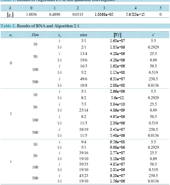
We also ran the regularized Newton algorithm (RNA) without correction, that is, we do not solve the linear equations (2.9)-(2.10) and just set the solution of (2.8) to be the trial step. Then, we tested the regularized New-ton algorithm without correction and Algorithm 2.1 for various of n, α_i and different choices of the starting point. The results are listed in Table 2. α_i: the selected value of α_i; Dim: the dimension n of the problem; x₀: the ith element x₀; niter: the number of iterations required; ∇f : the final value of ∇f x

( )

_k ; x*: the final value of x_k. We use

( )

5

10

k

f x −

[image:8.595.141.484.349.722.2]

∇ ≤ as the stopping criterion.

Table 1. Results of Algorithm 2.1 to test quadratic convergence.

k 0 1 2 3 4 5

k

g 1.8856 0.4890 0.0315 1.0368e−05 5.6523e−15 0

Table 2. Results of RNA and Algorithm 2.1.

i

α Dim x0 niter ∇f

*

x

0

10 i 3/1 1.63e−07 5.5

1/i 2/1 1.85e−06 0.2929

50 i 13/4 4.28e−06 25.5

1/i 19/6 4.28e−06 0.09

100 i 16/3 1.62e−06 50.5

1/i 5/2 1.15e−08 0.519

500 i 49/6 6.31e−07 250.5

1/i 18/8 2.08e−08 0.0136

1

10 i 5/1 2.66e−06 5.5

1/i 8/2 5.6e−12 0.2929

50 i 7/3 3.84e−10 25.5

1/i 25/14 4.86e−09 0.09

100 i 8/2 4.95e−06 50.5

1/i 11/5 2.30e−06 0.519

500 i 38/19 3.45e−07 250.5

1/i 11/5 5.48e−06 0.0136

i

10 i 9/4 9.56e−08 5.5

1/i 5/1 9.00e−06 0.2929

50 i 39/16 2.77e−07 25.5

1/i 19/10 3.10e−08 0.09

100 i 59/35 4.85e−07 50.5

1/i 19/10 2.81e−06 0.519

500 i 45/23 6.20e−07 250.5

(9)

Moreover, we can see for the same α_i, n and x₀, the number of iterations of Algorithm 2.1 is always less than that of RNA. And the correction term does help to improve RNA when the initial point is far away from the minimizer. These facts indicate that the introduction of correction is really useful and could accelerate the con-vergence of the regularized Newton method.

4. Concluding Remarks

In this paper, we propose a regularized Newton method with correction for unconstrained convex optimization. At every iteration, not only a RNM step is computed but also two correction steps are computed which make use of the previous available Jacobian instead of computing the new Jacobian. Numerical experiments suggest that the introduction of correction is really useful.

Acknowledgements

This research is supported by the National Natural Science Foundation of China (11426155) and the Hujiang Foundation of China (B14005).

References

[1] Yang, W.W., Yang, Y.T., Zhang, C.H. and Cao, M.Y. (2013) A Newton-Like Trust Region Method for Large-Scale Unconstrained Nonconvex Minimization. Abstract and Applied Analysis, 2013.

[2] Polyak, R.A. (2009) Regularized Newton Method for Unconstrained Convex Optimization. Mathematical Program-ming Series B, 120, 125-145. http://dx.doi.org/10.1007/s10107-007-0143-3

[3] Shen, C.G., Chen, X.D. and Liang, Y.M. (2012) A Regularized Newton Method for Degenerate Unconstrained Opti-mization Problems. Optimization Letters, 6, 1913-1933. http://dx.doi.org/10.1007/s11590-011-0386-z

[4] Sun, W. and Yuan, Y. (2006) Optimization Theory and Methods. Springer Science and Business Media, LLC, New York.

[5] Zhou, W. and Li, D. (2008) A Globally Convergent BFGS Method for Nonlinear Monotone Equations without Any merit Functions. Mathematics of Computation, 77, 2231-2240. http://dx.doi.org/10.1090/S0025-5718-08-02121-2

[6] Argyros, I.K. and Hilout, S. (2012) On the Convergence of Damped Newton Method. Applied Mathematics and Com-putation, 219, 2808-2824. http://dx.doi.org/10.1016/j.amc.2012.09.011

[7] Nashed, M.Z. and Chen, X. (1993) Convergence of Newton-Like Method for Singular Operator Equations Using Outer Inverses. Numerische Mathematik, 66, 235-257. http://dx.doi.org/10.1007/BF01385696

[8] Kelley, C.T. (1999) Iterative Methods for Optimization. In: Frontiers in Applied Mathematics, Vol. 18, SIAM, Phila-delphia, 2. http://dx.doi.org/10.1137/1.9781611970920

[9] Sun, D. (1999) A Regularization Newton Method for Solving Nonlinear Complementarity Problems. Applied Mathe-matics and Optimization, 40, 315-339. http://dx.doi.org/10.1007/s002459900128

[10] Li, D.H., Fukushima, M., Qi, L. and Yamashita, N. (2004) Regularized Newton Methods for Convex Minimization Problems with Singular Solutions. Computational Optimization and Applications, 28, 131-147.

http://dx.doi.org/10.1023/B:COAP.0000026881.96694.32

[11] Fan, J.Y. and Yuan, Y.X. (2005) On the Quadratic Convergence of the Levenberg-Marquardt Method without Non-singularity Assumption. Computing, 74, 23-39. http://dx.doi.org/10.1007/s00607-004-0083-1

[12] Fan, J.Y. and Pan, J.Y. (2009) A Note on the Levenberge-Marquardt Parameter. Applied Mathematics and Computa-tion, 207, 351-165. http://dx.doi.org/10.1016/j.amc.2008.10.056

[13] Fan, J.Y. and Yuan, Y.X. (2014) A Regularized Newton Method for Monotone Nonlinear Equations and Its Applica-tion. Optimization Methods and Software, 29, 102-119. http://dx.doi.org/10.1080/10556788.2012.746344

[14] Powell, M.J.D. (1975) Convergence Properties of a Class of Minimization Algorithms. In: Mangasarian, O.L., Meyer, R.R. and Robinson, S.M., Eds., Nonlinear Programming, Vol. 2, Academic Press, New York, 1-27.