Dynamical properties of a particle in a
time-dependent double-well potential
Edson D. Leonel and P.V.E. McClintock
Department of Physics, Lancaster University, Lancaster, LA1 4YB, United Kingdom
Abstract. Some chaotic properties of a classical particle interacting with a time-dependent double-square-well potential are studied. The dynamics of the system is characterised using a two-dimensional nonlinear area-preserving map. Scaling arguments are used to study the chaotic sea in the low energy domain. It is shown that the distributions of successive reflections and of corresponding successive reflection times obey power laws with the same exponent. If one or both wells move randomly, the particle experiences the phenomenon of Fermi acceleration in the sense that it has unlimited energy growth.
1. Introduction
The dynamics of systems interacting with time-dependent potentials has received close attention in theoretical and experimental physics over many years. In quantum systems, one interesting question is the tunnelling time through a potential barrier [1]. It is well known that it depends on the energy of the particle and the height of the potential, but the situation becomes much more complicated [2] when the height of the barrier is time-dependent. Considerable effort has been devoted to trying to understand such systems, including numerical studies of the transmission probability spectrum in a driven triple diode in the presence of a periodic external field [3], photon-assisted tunnelling through a GaAs/AlxGa1−xAs quantum dot induced by a microwave external frequency [4], sequential tunnelling in a superlattice induced by an intense electric field [5], transmission above a quantum well considering the effect of possible capture into a bound state in the well due to dissipation [6], and the probability of tunnelling in the presence of friction in Josephson junction circuits [7].
case of an infinite chain of oscillating square wells they showed that, although there is an intricate and complex dynamics, a chaotic orbit does not have unlimited energy gain. This is closely related to the fact that the phase space presents invariant spanning curves. A different version of this problem considering a classical particle interacting with an infinite box of potential that contains one oscillating square well was discussed in [11] using a formalism that could be interpreted as equivalent to studying the problem of a particle interacting with an oscillating square well with periodic boundary conditions; it could also be applied to the problem of an infinite chain of oscillating square wells. The authors found an abrupt transition in the Lyapunov exponent and suggested that it was due to destruction of the first invariant spanning curve and the consequent merging of different large chaotic regions.
It is also interesting to study problems where a classical particle interacts with a static or time-dependent multi-well potential in the presence of noise. Recent results include exact solutions for the problem of diffusion within static single and double square wells [12, 13], an introduction of external fields for a two-level system in a classical potential [14], a general solution of the problem of activated escape in periodically-driven systems [15], analytical solutions for the problem of a piecewise bistable potential in the limit of low external perturbation [16], the escape flux from a multi-well metastable potential preceding of the formation of quasi-equilibrium [17], activation over a randomly fluctuating barrier [18, 19], diffusion across a randomly fluctuating barrier [20] and diffusion of a particle in a piecewise potential in the presence of small fluctuations of the barriers [21]. The main result of this latter paper is that the flux of particle through the barrier may either increase or decrease, a result that is independent of the frequency of the oscillations.
The well known billiards problems are closely related. They consist basically of quantum or classical particles confined within closed boundaries with which they undergo elastic collisions [22, 23, 24, 25, 26], producing a variety of behaviours. Depending on the boundary and the control parameters, as well as on the initial conditions, it is possible to observe integrability, non-integrability, and ergodicity. The main question with a time-dependent boundary is whether or not the system exhibits the phenomenon of Fermi acceleration [27]. A more detailed discussion of this very interesting question together with specific examples can be found in Ref. [28] where the authors proposed the following conjecture: “chaotic dynamics of a billiard with fixed boundary is a sufficient condition for the Fermi acceleration in the system when a boundary perturbation is introduced”.
Depending on the energy, the particle may stay trapped in one well for some interval of time. We show that the time that the particle remains trapped in the well, also called the reflection time, obeys a distribution fitted by a power law that has the same exponent for both wells. This distribution is observed only for chaotic orbits located below the first invariant spanning curve. In a similar way, we have observed that for very specific values of the energy, the particle can exhibit the phenomenon ofresonance in which it exits the well with the same energy as it had on entry. As we will see, the introduction of random fluctuations in the depths of one or both wells confers unlimited energy growth on the particle.
The paper is organised as follows: in section 2, we describe in full detail all the steps used to construct the map. We present in Sec. 3 our results for the deterministic version of this problem, while Sec. 4 discusses the stochastic model. Finally, we summarise and and make our concluding remarks in Sec. 5.
2. The model with periodic oscillations
We consider the problem of a classical particle moving inside an infinite box of potential that contains two oscillating square wells. It could be related directly to mesoscopic systems [3] with time-dependent potentials [3, 6] with the square wells representing the conduction band for a heterostructure of GaAs/AlxGa1−xAs while the time-dependent potential could represent the electron-phonon interaction [29]. Furthermore, the formalism used to derive the scaling relation for the chaotic low energy region in this problem could be very useful and directly applicable to billiards problems. Such formalism was recently applied to the careful investigation of the chaotic sea in the Fermi-Ulam accelerator model [30].
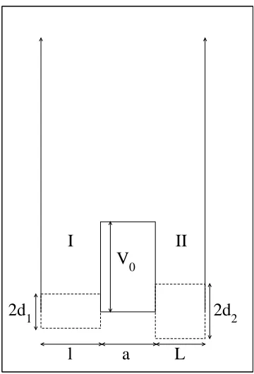
The problem relates to a typical one-dimensional system and may be described using the HamiltonianH(x, p, t) =p2/2m+V(x, t). HereV(x, t) describes the potential within which the particle must remain, which can be written as
V(x, t) =
⎧ ⎪ ⎪ ⎪ ⎪ ⎨ ⎪ ⎪ ⎪ ⎪ ⎩
∞ if x≤0 and x≥l+a+L
d1sin(ω1t) if 0< x < l
V0 if l≤x≤l+a
d2sin(ω2t) if l+a < x < l+a+L
2d1 2d2
l a L
V
0
[image:4.612.204.384.67.332.2]I II
Figure 1. Sketch of the potential V(x, t). The zero of x is in the bottom left-hand corner.
2.1. Map derivation
We now describe in detail the steps used in construction of the map. We adopt the same general procedures [9] recently applied [31] to the problem of a time modulated barrier. Suppose that the particle is atx=ltravelling to the left with total energyEn=Kn+V0 at time t=tn. As it enters well I, it experiences an abrupt change in its kinetic energy, and the new value is given by Kn =En−d1sin(ω1tn). Inside well I, the particle travels with constant velocity vn = 2[En−d1sin(ω1tn)]/m because there are no potential gradients. It undergoes an elastic collision with the wall at x= 0, and is reflected back. The time taken by the particle in travelling the distance 2listn= 2l/vn. When it arrives at x= l again, it will escape from well I only if En =Kn +d1sin[ω1(tn+tn)]> V0. If
En ≤V0, the particle is reflected inside well I, travels the distance 2l again, and so on.
It will escape from well I only when the following condition is satisfied
En =Kn +d1sin[ω1(tn+itn)]> V0 . (1)
time spent in this way above the barrier is tn = a/vn. On entry to well II, the particle again suffers an abrupt change in its kinetic energy and the new relation is
Kn = En −d2sin[ω2(tn+itn+tn)]. The velocity of the particle inside the well II is
vn =2Kn/m. When it reaches the right hand wall atx=l+a+L, it experiences an elastic collision and is reflected backwards at same velocity. So the time spent by the particle in travelling the distance 2L istn = 2L/vn. The particle will escape from well II ifEn+1 =Kn+d2sin[ω2(tn+itn +tn+tn)]> V0. But ifEn+1 ≤V0, the particle will be reflected again inside well II, travel the distanceLand, after suffering another elastic collision, will be reflected back again. It will escape from well II only if the following condition is fulfilled
En+1 =Kn+d2sin[ω2(tn+itn+tn+jtn)]> V0 , (2)
where j is the smallest integer for which equation (2) is true. Escaping from well II, the particle travels the distance a with velocity vv
n =
2(En+1−V0)/m in time
tv = a/vv until reaches the entrance of well I. The total time thus expended is
tn+1 =tn+itn+tn+jt+tv, so that the map T can be written as
T :
En+1 =Kn+d2sin[ω2(tn+itn+tn+jtn)]
tn+1 =tn+itn+tn+jt+tv
. (3)
Because of the way in which the map was derived, there are an excessive number of control parameters, 8 in total, including l, L, a, ω1, ω2, d1, d2 and V0. It is much more convenient to rewrite the map (3) in terms of dimensionless parameters, retaining only those that are relevant and effective. We use both normalised energy en = En/V0 and normalised amplitudes δ1 = d1/V0 and δ2 = d2/V0 of oscillation of the bottoms of the wells. A practical measure of time could be by counting the number of oscillations of well I, so that we can define the phaseφn=ω1tn. We define the ratio of the frequencies as r=ω2/ω1. It is also interesting to define the following parameter,
Nc =
m
2V0 2l
τ1 , (4)
whereτ1 = 2π/ω1 is the oscillation period of well I. The parameterNc then gives us the number of oscillations of well I during the length of time in which the particle travels distance 2l inside it at constant kinetic energy K = V0, in the absence of oscillations. Using these new variables, the map T can be rewritten as
T : ⎧ ⎪ ⎪ ⎪ ⎪ ⎨ ⎪ ⎪ ⎪ ⎪ ⎩
en+1 =en−δ1sin(φn) +δ1sin(φn+iΔφa)
−δ2sin[r(φn+iΔφa+ Δφb)]
+δ2sin[r(φn+iΔφa+ Δφb+jΔφc)]
φn+1 =φn+iΔφa+ Δφb+jΔφc + Δφd
, (5)
where the auxiliary variables are given by
Δφa = 2πNc
en−δ1sin(φn)
, Δφb = a
l
πNc
√
Δφc = L
l
2πNc
en−δ2sin[r(φn+iΔφa+ Δφb)]
,
Δφd= a
l
πNc
√
en+1−1 ,
i is the smallest integer for which equation (6) is true,
en=en−δ1sin(φn) +δ1sin(φn+iΔφa)>1 , (6)
and j is the smallest integer number for which equation (7) is true,
en+1 =en−δ2sin[r(φn+iΔφa+ Δφb)]
+ δ2sin[r(φn+iΔφa+ Δφb+jΔφc)]>1 . (7) This map is area-preserving because it possesses the property that detJ = 1, where J is its Jacobian matrix. Using these variables the map now has six dimensionless and effective control parameters namely δ1, δ2, Nc, r, a/l and L/l.
The case of synchronised oscillations (r = 1) of equal amplitude (δ1 = δ2) for symmetrical wells (L/l = 1) has already been studied [10, 11]. For the special case where the driving is also in-phase, the system must be related to the problem of a time-modulated barrier [8, 9] (see also [31] for recent results) because the relative movement of the different parts of the potential is then identical. As we will see, however, it is also of interest to investigate the dynamical properties in the more general cases that arise where the oscillations may be of unequal amplitude, not necessarily synchronised, and where the wells may be asymmetrical as well as symmetrical.
3. Numerical results
We now present and discuss our numerical results for the model defined in Sec. 2. The first step is choose appropriate control parameters and to start investigating the corresponding dynamical properties. We will consider first the symmetrical case and then, secondly, the asymmetrical one.
3.1. The symmetrical case
The symmetrical case consists basically in analysing the system specified bya/l=L/l= 1, such that each well and the barrier (see Fig. 1) are of the same width. Before choosing the value of the control parameter Nc, let us first discuss its physical significance. As originally defined (see eq. (4)), it gives information about the frequency of oscillation of well I, and we can rewrite it in a more appropriate form as Nc = tc/τ1. The time
tc = 2l
m/(2V0) gives the interval within which the particle travels the distance 2lwith kinetic energy K = V0. Related to this time, we can define a characteristic frequency
ωc = 2π/tc. Using such a relation, and a similar one for the period τ1, the control
0
1
2
3
4
5
6
φ
2
4
6
8
10
e
0
1
2
3
4
5
6
φ
2
4
6
8
10
e
(a)
[image:7.612.143.446.38.474.2](b)
Figure 2. Phase space for the mapT. The control parameters used werea/l=L/l= 1,Nc=G,δ1=δ2= 0.25, with: (a) r= 2; and (b)r= 3.
ofNc, we obtain thatω1 = 0.618. . . ωc, characterising the fact that well I oscillates with a frequency that is low compared toωc. Having defined the control parameters, we now construct the phase space for this model. Fig. 2 shows the phase spaces for (a) r = 2 and (b) r = 3 with a fixed amplitude of oscillation δ1 = δ2 = 0.25. They exhibit a very rich hierarchy of behaviours including KAM islands, invariant spanning curves and chaotic seas. We also see that variation of the control parameter r influences the shape of the phase space directly, changing the positions of the invariant spanning curves and KAM islands. An immediate consequence is that the shape of the chaotic sea is also modified. We will use Lyapunov exponent to characterise the chaotic sea.
0
1.5e+08
3e+08
4.5e+08
n
0.7
0.725
0.75
0.775
λ
0
1.5e+08
3e+08
4.5e+08
n
0.78
0.81
0.84
0.87
λ
(a)
[image:8.612.141.449.45.467.2](b)
Figure 3. Asymptotic convergence of the positive Lyapunov exponent for the chaotic sea. The control parameters used werea/l=L/l= 1, Nc =G, δ1=δ2= 0.25with: (a)r= 2; and (b) r= 3.
rate of expansion or contraction of nearby initial conditions in the phase space. In this sense, negative exponents mean convergence of two slightly different initial conditions, whereas a positive Lyapunov exponent implies their divergence. If two initial conditions diverge exponentially in time, the system presents a chaotic component and the orbit is said to be chaotic. Periodic or quasi-periodic behaviour is characterised by negative Lyapunov exponents. We use the algorithm of triangularisation proposed by Eckmann and Ruelle [33] to evaluate the Lyapunov exponents. They are defined as
λj = limn→∞ n
k=1
1
nln|Λ
k
1
10
100
1000
10000
r
0.8
1.2
1.6
2
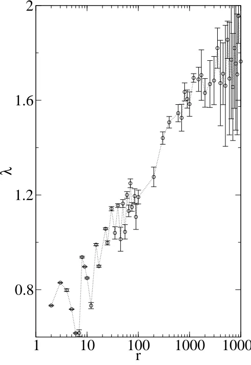
[image:9.612.166.411.46.403.2]λ
Figure 4. Positive Lyapunov exponent, λas a function ofr for the chaotic sea. The control parameters used werea/l=L/l= 1,Nc=Gandδ1=δ2= 0.25.
where Λk
j are the eigenvalues of M =
n
k=1Jk(ek, φk) and Jk is the Jacobian matrix
evaluated on the orbit (ek, φk). In order to calculate the eigenvalues of M, we use the fact that J can be written as the product J = ΘT, where Θ is an orthogonal matrix and T is a triangular one. We now define the elements of these matrices as
Θ =
cos(θ) −sin(θ) sin(θ) cos(θ)
, T =
T11 T12
0 T22
.
Introducing the identity operator, we rewrite M = JnJn−1. . . J2Θ1Θ−11 J1, and thus define Θ−11 J1 = T1. The product J2Θ1 defines a new matrix J2∗. As a next step, we may then write M =JnJn−1. . . J3Θ2Θ−12 J2∗T1. The same procedure yieldsT2 = Θ−12 J2∗. The problem is thus reduced to the evaluation of the diagonal elements of Ti :T11i , T22i . Using the Θ and T matrices, we find the eigenvalues of M, given by
T11 = j 2 11+j212
j112 +j212
, T22= j11j22−j12j21
j112 +j212
We can then evaluate the Lyapunov exponent using the relation
λj = limn→∞ n
k=1
1
nln|T
k
j|, j = 1,2.
The Lyapunov exponents possesses the property λ1 =−λ2 because the map T is area-preserving. Fig. 3 shows the convergence of the positive Lyapunov exponent from 5 different initial conditions for the chaotic low energy regions shown in Fig. 2. Each initial condition was iterated 5×10⁸ times to guarantee that the asymptotic value has been reached. The ensemble average of the five samples is: (a) λ = 0.733 ±0.001 and (b) λ = 0.831 ±0.002. We also obtain the behaviour of the positive Lyapunov exponent for the chaotic low energy region as function of r, as shown in Fig. 4 for control parameters a/l =L/l = 1, Nc =G and δ1 =δ2 = 0.25. Because of the change in the shape of the chaotic sea caused by variation ofr, and in particular the position of the first invariant spanning curve, the asymptotic convergence of the positive Lyapunov exponent requires progressively longer runs in order to approach its asymptotic value as r increases. Equivalently, with a fixed maximum iteration number nmax = 5×10⁸, the error bars for large values ofr are bigger than for those for smallr.
Let now us discuss some scaling properties for this model in the region related to the chaotic sea. We choose to characterise the behaviour in terms of the variance of the average energy, which we will refer to it as theroughness ω[34]. The procedure adopted here has already been used to characterise the chaotic low energy region of the Fermi-Ulam accelerator model [30] and to investigate scaling present in the chaotic sea for a time-modulated barrier [31]. Given the large number of control parameters present in this model, we will shall consider the following parameters to be fixed: a/l =L/l = 1;
δ1 = δ2 = 0.25; r = G (unsynchronised case). We then study the behaviour of the
roughness as function of the parameter Nc. To define the roughness we must first consider the average of the energy over the orbit generated from one initial condition
e(n, Nc) = 1
n
n
i=0
ei , (8)
and then evaluate the interface width around this average energy. We can thus define the roughness formally, considering an ensemble of B different initial conditions, as
ω(n, Nc)≡ 1
B
B
j=1
e2j(n, Nc)−e2j(n, Nc)
. (9)
An ensemble of initial conditions is used to smooth the roughness evolution, for which a typical curve is shown in Fig. 5(a); it was constructed by fixing the initial energy at
e0 = 1.001 and then ensemble-averaging 5,000 different initial phases in the interval
φ0 ∈ [0,2π), all of which gave rise to chaotic behaviour. The main idea of averaging
1
100
10000
1e+06
n
0.1
1
10
100
ω
1.002e-07
1.005e-07
1/n
91.22
91.24
91.26
ω
Numerical Data
Linear fit
a
b
n
xI
[image:11.612.151.446.41.451.2]II
β
Figure 5. (a) Roughness evolution for an ensemble of 5,000 different initial phases and same the initial energy e0 = 1.001, all of them leading to chaotic behaviour. (b) Procedure used to extrapolate the roughness after application of the transformation
n→1/n. The values of control parameters werea/l=L/l= 1,δ1=δ2= 0.25,r=G
andNc= 3000.
the iteration number increases, the roughness eventually bends towards the direction of a saturation regime that is obtained only for long enough iteration number (see below the details used to extrapolate the saturation of the roughness). The changeover from growth to convergence on saturation is characterised by a crossover iteration number
nx. It is well known that the chaotic sea is limited by the first invariant spanning
spanning curve changes. For the range of Nc over which we will investigate scaling in the roughness, an increase in Nc implies a rise in the position of the first invariant spanning curve so that, as a consequence, the roughness saturates at a higher value. We can then start to characterise the roughness scaling, supposing that:
(i) After the brief initial transient, the roughness grows as function of iteration number according to
ω(n, Nc)∝nβ. (10)
This growth can be seen in region I of Fig. 5. β is called the growth exponent. Equation (10) is valid for nnx.
(ii) As the iteration number increases, the roughness reaches saturation, as can be seen in region II of Fig. 5. The behaviour of the roughness within the saturation regime follows the equation
ωsat(Nc)∝Ncα, (11)
where α is the roughening exponent. Equation (11) is only valid forn nx. (iii) The crossover iteration number nx that tells us when the roughness growth slows
and saturation is being approached is given by
nx(Nc)∝Ncz (12)
where z is called the dynamical exponent.
We now summarise the procedure adopted to obtain the saturation value. Even for our maximum iteration number (n ≈500nx), we can see from the numerical simulations that growth of the roughness has not quite reached saturation. But if we choose to increase the maximum iteration number even more, this carries the disadvantage of leading to very much longer simulations. We therefore take the option of finding the saturation value by extrapolation. We apply the transformationn →1/n for the iteration number, which is applicable because the saturation grows slowly and linearly for sufficiently large values of n, yielding
ω(n, Nc) =ωsat(Nc) + const.
n . (13)
Considering the case of n → ∞, it is easy to see that Eq. (13) gives us that
ω(n, Nc) → ωsat(Nc), which may be obtained after doing a linear fit to the results. The procedure is illustrated in Fig. 5(b).
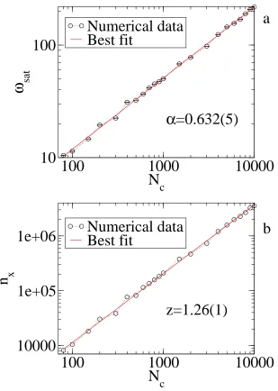
Next we discuss how to obtain the exponents α and z. The intercept of the power law (see Fig. 5(a)) with the linear coefficient obtained from Eq. (13) gives the crossover iteration numbernx. The exponentsαandz are then obtained from the graphs ofn(Nc) and ωsat(Nc) as shown in Fig. 6. Applying the power law fit, we find that α= 0.632(5) and z = 1.26(1). Obtaining β by averaging over all curves in the range of Fig. 6, we find β = 0.500(2).
100
1000
10000
N
c10
100
ω
satNumerical data
Best fit
100
1000
10000
N
c10000
1e+05
1e+06
n
xNumerical data
Best fit
a
b
α
=0.632(5)
[image:13.612.144.453.39.473.2]z=1.26(1)
Figure 6. (a) Roughness saturation ωsat and (b) crossover iteration number nx as functions of the control parameterNc. A power law fit gives us thatα= 0.632(5)and
z= 1.26(1).
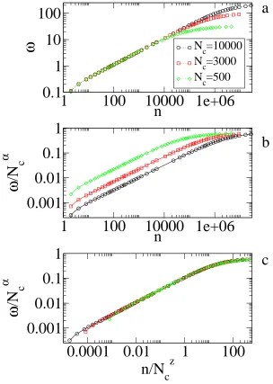
relocates all curves to the same saturation value, as shown in Fig. 7(b). The second step is to relocate all the curves to the same crossover iteration number, which is done by taking the ratio n/nx as shown in Fig. 7(c).
The success of this procedure for obtaining a universal plot for the roughness allows us to describe it using the following scaling function
ω(n, Nc) =ζω(ζbn, ζcNc), (14) where ζ is the scaling factor. We can then chooseζ =n−1b and rewrite Eq. (14) as
1
100
10000 1e+06
n
0.1
1
10
100
ω
N
c=10000
N
c=3000
N
c=500
1
100
10000 1e+06
n
0.001
0.01
0.1
1
ω
/N
c
α
0.0001 0.01
1
100
n/N
cz0.001
0.01
0.1
1
ω
/N
c
α
a
b
[image:14.612.146.450.50.477.2]c
Figure 7. (a) Roughness evolution for different values of Nc. (b) Collapse of the curves onto the same saturation value. (c) Collapse of the curves onto the same saturation value and same crossover iteration number.
The function ω1(n−cbNc) = ω(1, n−cbNc) is assumed constant for n nx. Considering Eq. (10) we obtain
n−1b =nβ ,
and β =−1/b. From our numerical simulations we have β = 0.500(2). Our second choice is ζ =N−1c
c and we have that
ω(n, Nc) =N−1c
c ω2(N−
b c
c n),
where the function ω2(N−bc
c n) = ω(1, N−
b c
Using Eq. (11) we obtain that
N−1c
c =Ncα ,
with α=−1/c.
Using the two previous relations together with the scaling factor and the corresponding relations for the exponents b andc, it is easy to show that the exponents
α, β and z are mutually connected by the following relationship
z = α
β . (15)
Evaluating Eq. (15) with our numerical results for α and β, we find that z = 1.264(5), which is gratifyingly close to the result obtained in Fig. 6(b).
3.2. The asymmetrical case
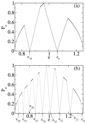
We now discuss a resonance phenomenon that manifests in the chaotic sea. It depends specifically on the energy of the particle immediately after it enters a well, and it may occur in either of the wells (see also Ref. [31] for a fuller discussion of resonances in the problem of a time modulated barrier). Entering the well, the corresponding range of energy where the resonance can take place is: (a) well I,e∈[eI
min, eImax] and (b) well II,
e∈[eII
min, eIImax] whereeImin = 1−δ1,eImax= 1 +δ1, eIImin = 1−δ2 andeIImax= 1 +δ2. The
resonances can be determined directly from the length of time that the particle spends travelling inside each well. For well I, this time is
Δφa= 2πNc
en−δ1sin(φn)
,
and for well II it is
Δφc = L
l
2πNc
en−δ2sin[r(φn+iΔφa+ Δφb)]
.
If either of these times is a multiple of 2π, the particle will not remain trapped within the corresponding well. From the range of energy within the relevant well, we can estimate the number of oscillations, the resonance energy, and the time of flight. The corresponding maximum and minimum values for the number of oscillations are given by: (a) well I,kI
max=Nc/
eI
min andkminI =Nc/
eI
max; (b) well II, kIImax = Ll√NeIIc min
and
kII min = Ll
Nc
√
eIImax
. After obtaining the range ofk values, the respective resonance energies for the two wells II are
eIk = N
2
c
k2 , e
II
k =
L
l
2 N2
c
k2 .
To illustrate the occurrence of such resonances, we choose to characterise the synchronised case (r = 1) and asymmetric case a/l = 1, L/l = 2.5 by different amplitudes of oscillation, δ1 = 0.25, δ2 = 0.35 for Nc = 15G. The latter value of
0.8
1
1.2
e
0
0.2
0.4
0.6
0.8
1
P
e0.8
1
1.2
0
0.2
0.4
0.6
0.8
1
0.8
1
1.2
e
0
0.2
0.4
0.6
0.8
1
P
e0.8
1
1.2
0
0.2
0.4
0.6
0.8
1
(a)
(b)
e
9e
10e
20e
22e
23e
24e
25e
26e
27 [image:16.612.150.441.43.465.2]e
28e
21Figure 8. Normalised distribution of successive reflection energies for the control parametersr= 1,a/l= 1,L/l= 2.5,δ1= 0.25,δ2= 0.35andNc = 15Gfor (a) well I and (b) well II.
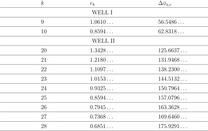
k ek Δφa,c
WELL I
9 1.0610. . . 56.5486. . . 10 0.8594. . . 62.8318. . .
WELL II
[image:17.612.77.507.42.312.2]20 1.3428. . . 125.6637. . . 21 1.2180. . . 131.9468. . . 22 1.1097. . . 138.2300. . . 23 1.0153. . . 144.5132. . . 24 0.9325. . . 150.7964. . . 25 0.8594. . . 157.0796. . . 26 0.7945. . . 163.3628. . . 27 0.7368. . . 169.6460. . . 28 0.6851. . . 175.9291. . .
Table 1. Resonance energies and flight times inside both well I and well II for the control parametersr= 1,a/l= 1,L/l= 2.5,δ1= 0.25,δ2= 0.35 andNc= 15G.
energy to escape. We now consider this case.
We discussed in Sec. 2 how, depending on the energy of the particle as it enters the well, it can stay trapped there while suffering successive reflections. After some interval of time, however, after satisfying some specific conditions, it will exit the well, and evolve inside the system (mainly in chaotic behaviour) until it again becomes trapped, not necessarily in the same well. In this way, we can characterise the distribution of successive reflections as well as the length of time during which the particle stays trapped in the well. It is expected that very long times (i.e. large number of successive reflections) should be observed less commonly than short times (small numbers of successive reflections). To characterise such behaviour, we choose the following combination of control parameters: the asymmetric case (a/l = 10), (L/l= 3) considering non-synchronised oscillations (r=G and Nc = 15G) of differing amplitude
δ1 = 0.25 and δ2 = 0.35. Fig. 9 shows the distributions of successive reflections, Pn,
and corresponding successive reflection times, Pt, for well I (a similar result is in fact also observed for well II). The analysis of Fig. 9 allows us to describe such distributions as Pn ∝ tγn and P
t ∝ tγt. After performing a power law fit, we obtain for well I that:
γn = −2.99(1) and γt = −3.00(2). A similar analysis for well II yields γn =−3.00(1)
1
10
100
1000
n
1
100
10000
1e+06
1e+08
P
n1
10
100
1000
t
100
10000
1e+06
1e+08
P
t(a)
[image:18.612.138.448.43.472.2](b)
Figure 9. (a) Distribution of successive reflections, Pn, and (b) successive reflection times Pt obtained for well I. The values of control parameters used were a/l = 10,
L/l= 3, r =G,Nc = 15G, δ1 = 0.25 and δ2 = 0.35. A power law fit gives us that
γn =−2.99(1)andγt=−3.00(2).
barrier [8, 9] and for a well beside a time-dependent barrier [31], and accounted for analytically in the case of a particle moving within a random well [11].
4. The stochastic model
numbers uniformly distributed between [−1,1] with the property that fk= 0. Using this formalism, the map T is written as
T : ⎧ ⎪ ⎪ ⎪ ⎪ ⎨ ⎪ ⎪ ⎪ ⎪ ⎩
en+1 =en−δ1f1(tn) +δ1f1(tn+iΔta)
−δ2f2[r(tn+iΔta+ Δtb)]
+δ2f2[r(tn+iΔta+ Δtb+jΔtc)]
tn+1 =tn+iΔta+ Δtb+jΔtc+ Δtd
,
where the auxiliary variables are given by
Δta= 2πNc
en−δ1f1(tn)
, Δtb = a
l
πNc
√
en−1 ,
Δtc = L
l
2πNc
en−δ2f2[r(tn+iΔta+ Δtb)]
,
Δtd= a
l
πNc
√
en+1−1 ,
i is the smallest integer number for which the following equation is true
en=en−δ1f1(tn) +δ1f1(tn+iΔta)>1 ,
and j is the smallest integer number that makes true the equation
en+1 =en−δ2f2[r(tn+iΔta+ Δtb)]
+δ2f2[r(tn+iΔta+ Δtb +jΔtc)]>1 .
We consider three different kind of stochastic perturbation to this system:
(1) Well I is periodic and well II moves randomly. In this situation, f1(t) = sin(t) and
f2(t) give uncorrelated random numbers.
(2) Well II is periodic and well I moves randomly. With these conditions, f1(t) give uncorrelated random numbers and f2(t) = sin(rt).
(3) Wells I and II both move randomly, i.e. f1(t) and f2(t) both give uncorrelated random numbers, and in addition, function f1(t) and f2(t) are mutually uncorrelated.
The introduction of the stochastic perturbation affects directly the complex structure of the phase space. In particular, for the range of control parameters used, it is possible to observe unlimited energy growth in the time evolution of the particle. To make evident this behaviour, we evaluate the following observables
¯
e= 1
B B i=1 ⎡ ⎣1 n n j=1 ej,i ⎤
⎦ , ¯t = 1
B B i=1 ⎡ ⎣1 n n j=1 tj,i ⎤
⎦ . (16)
0
5e+06
1e+07
n
0
150
300
450
Energy
Simulation
Best Fit
0
5e+06
1e+07
t
0
150
300
450
Energy
Simulation
Best Fit
(a)
[image:20.612.143.446.47.463.2](b)
Figure 10. Behaviour of the average energy as function of (a) iteration number n and (b) average time ¯t for the case where f1(t) is random and f2(t) is periodic. The control parameters used were Nc =r =G, δ1 =δ2 = 0.25, a/l=L/l = 1. A power law fit gives thatδn= 0.498(3)andδt= 0.647(2).
initial condition is sufficient to provide evidence for such growth, averaging over an ensemble of initial conditions makes the energy curve smoother and much easier to characterise. Fig. 10 shows the behaviour of ¯e(n) and ¯e(¯t). The control parameters used werea/l =L/l = 1,r =G, δ1 =δ2 = 0.25 and Nc =G. Similar results can be obtained for other combinations of control parameters. We use an ensemble of 10,000 different initial conditions, starting with an initial energy e0 = 1.001 and different initial seeds for the random number generator. Each initial condition was iterated 107 times. The analysis of Fig. 10 allow us to describe the growth of the energy as: (a) ¯e∝nδn and (b)
¯
our results shows that δn = 0.498(3) and δt = 0.647(2) (as in Fig. 10). For the case where well I is periodic and well II behaves randomly, we obtain that δn = 0.496(4) and δt = 0.644(7). Finally, considering the case where both wells behaves randomly, a power law fit givesδn = 0.497(4) andδt= 0.648(3). We can see that both exponents are robust, in the sense that they are independent of which well (I, or II, or both) is behaving randomly. The averages of the latter three exponents are given by ¯δn = 0.497(4) and ¯
δt = 0.646(4). It is especially gratifyingly that the exponent ¯δn has the same value as
that obtained from a random walk, given that the dynamics is essentially the same. In an attempt to account for the difference between the exponents ¯δn and ¯δt we point out that, during a given interval, a particle with high energy can iterate many more times within a well than a particle with low energy. The authors of [28] conjectured that Fermi acceleration should be observed for a billiard with a time-dependent boundary if the corresponding version for a fixed boundary presents chaotic components. However, we can conclude that for the system studied in the present paper (see also [11] and [31] for comparable results in other systems) which exhibits chaotic behaviour under a time-dependent (periodic) perturbation, Fermi acceleration is observed only after the introduction of random (stochastic) motion to the time dependent potential.
5. Final remarks and conclusions
We have studied the problem of a classical particle inside an infinite box of potential that contains two time-dependent square wells. We describe this problem via the formalism of a discrete map, considering two types of time dependence: (i) periodic and (ii) stochastic. For the periodic dependence we discuss results for both the symmetrical and asymmetrical cases, as well as for both the synchronised and unsynchronised cases. We concentrate on the chaotic low energy region, which we characterise in terms of Lyapunov exponents. We derive a scaling relation for the variance of the average velocity (roughness) and show that the critical exponents obeys an analytic relationship. In the low energy region, the particle may stay temporarily trapped in the time-dependent well. We shown that the distributions of successive reflection numbers and successive reflection times obey power laws with the same exponent. The particle may also experience the phenomenon of resonance, i.e. it may exit the well with same energy as it had when it entered. For the case in which one or both wells move randomly, we have shown that the particle exhibits growth in velocity and correspondingly in kinetic energy. Such behaviour is clear evidence of the Fermi acceleration phenomenon.
Acknowledgements
References
[1] Cohen-Tannoudji C, Diu B and Lalo¨e F 1977 Quantum Mechanics Vol I (Wiley New York); Gasiorowicz S 1974Quantum Physics(Wiley New York)
[2] B¨utiker M and Landauer R 1982Phys. Rev. Lett.491739 [3] Wagner M 1998Phys. Rev. B.5711899
[4] Kouwenhoven L P, Jauhar S, Orenstein J, McEuen P L, Nagamune Y, Motohisa J and Sakaki H 1994Phys. Rev. Lett.733443
[5] Guimar˜aes P S S, Keay B J, Kaminski J P, Allen Jr S J, Hopkins P F, Gossard A C, Florez L T and Harbison J P 1993 Phys. Rev. Lett.70 3792
[6] Cai W, Hu P, Zheng T F, Yudanin B and Lax M 1990Phys. Rev. B.413513 [7] Caldeira A O and Leggett A J 1981Phys. Rev. Lett.46211
[8] Mateos J L and Jos´e J V 1998 Physica A257434 [9] Mateos J L 1999Phys. Lett. A256113
[10] Luna-Acosta G A, Orellana-Rivadeneyra G, Mendoza-Galv´an A and Jung C 2001Chaos, Solitons and Fractals12 349
[11] Leonel E D and da Silva J K L 2003Physica A323181 [12] Berdichevsky V and Gitterman M 1996Phys. Rev. E531250
[13] Berdichevsky V and Gitterman M 1996J. Phys. A: Math. Gen.291567 [14] Berdichevsky V and Gitterman M 1999Phys. Rev. E59R9
[15] Dykman M I, Golding B, McCann L I, Smelyanskiy V N, Luchinsky D G, Mannella R and McClintock P V E 2001 Chaos11 587
[16] Berdichevsky V and Gitterman M 1996J. Phys. A: Math. Gen.29L447
[17] Array´as M, Kaufman I Kh, Luchinsky D G, McClintock P V E, Soskin S M 2000Phys. Rev. Lett.
842556
[18] Iwaniszewski J 2003Phys. Rev. E68027105
[19] Iwaniszewski J, Kaufman I Kh, McClintock P V E, McKane A J 2000Phys. Rev. E611170 [20] Iwaniszewski J 1996Phys. Rev. E543173
[21] Berdichevsky V and Gitterman M 1999Phys. Rev. E607562 [22] Karner G 1994Journal of Stat. Phys.77867
[23] Seba P 1990Phys. Rev. A41 2306
[24] Tsang K Y and Ngai K L 1997Phys. Rev. E56R17 [25] Berry M V 1981Eur. J. Phys.291
[26] Robnik M and Berry M V 1985J. Phys. A181361 [27] Fermi E 1949Phys. Rev.751169
[28] Loskutov A, Ryabov A B and Akinshin L G 2000J. Phys. A: Math. Gen.337973 [29] Cai W, Zheng T F, Hu P, Yudanin B and Lax M 1989Phys. Rev. Lett.63418 [30] Leonel E D, McClintock P V E and da Silva J K L 2004Phys. Rev. Lett.9314101 [31] Leonel E D and McClintock P V E 2004Phys. Rev. E70 16214
[32] Lichtenberg A J and Lieberman M A 1992 Regular and Chaotic Dynamics (Appl. Math. Sci.38 Springer Verlag New York)
[33] Eckmann J -P and Ruelle D 1985Rev. Mod. Phys.57617