Parallel algorithm based on Fast Fourier transforms

Journal of Chemical and Pharmaceutical Research, 2014, 6(3):188-195

Research Article

_{CODEN(USA) : JCPRC5}

ISSN : 0975-7384

Parallel algorithm based on Fast Fourier transforms

Yuhuan Cui

*

_{, Jingguo Qu and Guanchen Zhou}

Qinggong College, Heibei United University, Tangshan, China

_____________________________________________________________________________________________

ABSTRACT

Digital signal processing technology over the last decade with the digital computer, large scale integrated circuits and other advanced technologies, with rapid advances, has formed a strong technical and scientific vitality. Because it itself has a range of advantage, so effective in promoting the field of engineering technology transformation and subject development, more extensive application fields, in-depth, more and more people's attention. First, the fast Fourier transform (FFT) digital signal processing is the most basic computing, this article describes the beginning of the fast Fourier transform definition and the most widely used types. Then, the definition of parallel algorithms and matrix operations and matrix multiplication parallel algorithms parallel algorithms, parallel algorithms are also introduced performance metrics. Finally, a practical application, reflects the fast Fourier transform algorithm used in parallel, through the main parallel FFT algorithm is studied, expect that the parallel Fast Fourier Transform algorithm has a clear understanding.

Keywords:Digital signal processing; Fast Fourier transform; Parallel algorithm; FPGA

_____________________________________________________________________________________________

INTRODUCTION

So far, FFT algorithm has development for 30 years, in 1965, the first time before the Fast Fourier Transform (FFT) algorithm proposed. The application of Discrete Fourier Transform (DFT) has been difficult to expand. Because of FFT is proposed, make the realization of DFT becomes closer to reality. DFT applications are also expanding rapidly [1].

In digital signal processing DFT is the transform approach used in common. It plays an important role in a variety of digital signal processing systems. The history of Fourier transform is about one hundred years, we know that the frequency-domain analysis is often better than the time-domain analysis. It is not only simple, and easy to analyze complex signals. But use numerical methods with more accurate, that is DFT spectral analysis. Appear before the FFT is impractical, because the calculation of DFT is too big. FFT is not another transformation that different from DFT. It is a fast and effective algorithm to reduce calculation times of DFT.

FFT considers the constraints to achieve the computer and digital hardware .study on the operational structure for machine operation, the DFT computing time is shortened by 1 to 2 orders of magnitude，It can effectively reduce the storage capacity required，it can reduce the capacity required of storage effectively.

2. Fast Fourier Transform 2.1. Definition of the FFT

When calculate the signal sequence of

x n

( )

do a discrete Fourier transform, the direct transformation is

 

1

0

( )

0,1, 2,...,

1

N

nk N n

X k



x n W

k

N











(1)

The inverse transformation is

 

1

 

0

1

0,1, 2,...,

1

N

nk N n

x n

X k W

n

N

N













(2)

Where

W

_N



e

j2/N,

x

 

n

and

X

 

k

type can be real or complex. Seen from the above equation, to calculate a sample sequence is N times to do complex multiplication and n-1 time’s complex adder.

The basic idea of ​​FFT algorithm design, it is to make full use of the periodicity and symmetry of DFT, reduce duplication of calculation, and make the N-point long sequence into several short sequences, reducing the length of each sequence, can greatly reduce the amount of calculation [2].

The signal sequence of length is

N



2

M , which,

M

is positive integer, the time domain signal sequence, even part of the

x

 

2

n

and the odd part of

x



2

n



1



, among

1

2

,...,

2

,

1

,

0





N

n

, Then the discrete Fourier transform signal sequence of A can use the discrete Fouriertransform of two B sampling points are represented and calculation. Considering A and the periodicity of discrete Fourier transform. Formula (1) can be written as

 

2 1

 

2 1





 

 

0 2 0 2

2

2

1

N N

nk k nk k

N N N N

n n

X k

x n W

W

x n

W

G k

W H k

 

 















(3)

Among

 

2 1

 

0 2

2

N nk N n

G k

x n W









(4a)

 

2 1





0 2

2

1

N nk N n

H k

x n

W











(4b)

Thus, Formula (4) is the two discrete Fourier transform that contains only A points of the discrete Fourier transform,

 

k

G

includes only the even number sequence of original signal sequence, A includes only the odd point sequence. Though

k



0

,

1

,

2

,...,

N



1

, but the cycle of

G

 

k

and

H

 

k

is

N

/

2

. Their value to

N

/

2

cycle is repeated.

Because

2

/2 2

₁

N j N N N

W

e

    _ _



 

. So, _Nk

N k

N

W

W

2





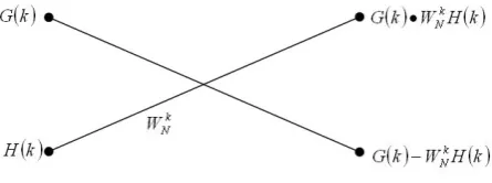
_{. So by the formula (3) and (4) to get}

 

 

 

0,1, 2,...,

1

2

k N

N

X k



G k



W H k

k





(5a)

 

 

2

k N

N

X k



_





_



G k



W H k





(5b)

[image:3.595.198.421.82.165.2]

Figure 1 Butterfly Fast Fourier Transform

Commonly used signal butterfly algorithm flow chart representation (5) of the discrete Fourier transform.

2.2. Frequency extraction algorithm

According to the frequency of extraction FFT algorithm. The algorithm is a frequency-domain signal is decomposed into a sequence of parity

X k

( )

in two parts, but the algorithm is still sequential operation start signal from a time domain sequence, the same is divided into the point

N

,

N

2

calculated points FFT, can directly calculate the discrete Fourier transform

N

2multiplications needed to be reduced to

N

log

₂

N

2



times.

In the case of

N



2

before and after the point input sequence

N

,

x n

( )

into two halves

 

 

 

1

2

0,1, 2,...,

1

2

2

x n

x l

N

l

N

x n

x l







_

_



_



_









_

_



(6)

1

( )

2

( )

x n



x n

is the length of time series

N

2

, so the point discrete Fourier transform can be written as

N

.

 

2 1 1

 

2

 

0 2

2

N

nl N n

X

l

x n

x n W











_





_

(7a)





2 1 1

 

2

 

0 2

2

1

N

k nl

N N

n

X

l

x n

x n W W





 





_





_



(7b)

Frequency signal sequence

X l

(2 )

is

N

2

discrete Fourier transform of the time signal sequence

x n

₁

( )



x n

₂

( )

, Frequency signal sequence

X l

(2



1)

is

N

2

discrete Fourier transform of the time signal sequence



x n

₁

( )



x n W

₂

( )



_Nn, therefore,

Calculation of the point

N

discrete Fourier transform, through the two plus (minus) method and one multiplication, obtain two sub sequences from the original sequences, so, Frequency extraction algorithm also has butterfly form. The base 2 FFT butterfly basic formula is:

 

 

 

 

 

 

1 2

1 2

0,1, 2,...,

1

2

n N

a n

x n

x n

_N

n

b n

x n

x n W







_

_



















(8)

The computation is same as the time extraction algorithm completely. That is, it just needs

N

log

₂

N

multiplications and

N

log

₂

N

plus (minus) method operation

3. Parallel Algorithms

Algorithms in the climax, the 1970s to the 1980s; To the 1990s hit bottom; currently, they are in the hot phase of the study. Now, people can build their own PC cluster, to solve practical problems.

3.1. Parallel matrix multiplication algorithm

The definition and calculation structure of matrix multiplication are very simple, but the amount of calculation is large, the computational complexity of

n

order matrix multiplication serial is

2

n

3



n

2 . In order to save computation, there are such as Strassen, Winograd, V.Pan and other fast matrix multiplication, among, Calculate the amount of the proposed algorithm by V.Pan had dropped to

O



n

2.496



, unfortunately, the parallelism of many fast matrix multiplications are not very good. Not easy to implement on parallel computers.

Set up

A



 

a

_ij is

m



n

order matrix,

B



 

b

_ij is

n



p

order matrix, its product

C



 

c

_ij is

m



p

order matrix [4]:







n

k kj ik

ij

a

b

c

1

m

i



1

,

2

,

3

,



,

，

j



1

,

2

,

3

,



,

p

（9）

A parallel algorithm of matrix multiplication commonly used has two kinds: inner product algorithm and outer product algorithm.

Inner product algorithm refers to the formula (9) in two n-dimensional vector inner product forms. That is





_









_{i i in j j nj}

ij

a

a

a

b

b

b

c

₁

,

₂

,



,

₁

,

₂

,



,

According to the formula calculated for parallel matrix multiplication algorithm called the inner product, It is generally used

n

processors. With a multiplicative calculated all

a

_ik



b

_kj for

k



1

,

2

,



,

n

Do



log

₂

n



additions can find

c

_ij.

There are two outer product algorithms; one is the column vector notation of the matrix

C





_







 

_



n

k k k mk kj

mj j

j

j

c

c

c

a

a

a

b

C

1 1 2

2 1

*

,

,



,

,

,



,

,

j



1

,

2

,

3

,



,

p

The

j

columns of

C

matrix is

C

*_j

Where

C

*_j refers to the first row

j

,

C

matrix. It is used when the number of processors is

p

，

j

units respectively by the first processor calculates the first row vectors

j

of

C

.

Where

C

_i* refers to the first row

i

,

C

matrix. It is used when the number of processors is

m

，

i

units respectively by the first processor calculates the first row vectors

i

of

C

. Matrix multiplication parallel algorithm in an outer product in the process of calculation, a row or column element of each node machine at least

C

calculation. Compared to the inner product algorithm, the task granularity is bigger, the parallel computation of computation and communication of the relatively large, distributed system which is suitable for loosely coupled.

3.2. Parallel algorithm performance metrics

For a given problem, we need to evaluate the performance of parallel algorithms, parallel algorithms to determine which meets our needs. We will measure the performance of a number of parallel algorithms are introduced, such as speedup and efficiency of the algorithm running time and the degree of parallelism and algorithms [5].

3.2.1 Running time

3.2.2 Parallelism

Algorithm parallelism (Degree of Parallelism, DOP) is the number of operation of the algorithm can be executed in parallel. Few parallel algorithms can maintain the same degree of parallelism during the execution of the algorithm, and therefore more accurate to say they should add time constraints, namely the degree of parallelism within a certain time frame. From the intuitive sense, the amount of parallelism is portrayed "degree of parallelism" in a parallel algorithm, which reflects the degree of parallelism in the software and hardware parallelism match.

And algorithms related to the concept of parallelism granularity, in general, a large particle size means that independent parallel execution of tasks large and small algorithm parallelism; Small particle size means that small independent parallel execution of tasks, parallel algorithm is large. The average degree of parallelism parallel algorithms can be defined as: Assuming parallel algorithm can be done in parallel within the

m

-step, the degree of parallelism of the algorithm when the step is

DOP

 

l

, the average degree of parallelism of the algorithm

 







m

l

l

DOP

m

A

1

1

3.2.3 Speedup and efficiency

Speedup of parallel algorithm is defined as:

p p

T

T

S

_

1 _{，Among them,} 1

T

is the optimal serial algorithm running

time on a single processor;

T

_prefers to the time required for parallel algorithms in parallel processor computer using the

p

units. Not difficult to see,p bigger the better.The ideal case

S

p



P

. But actually, only similar to the very

special circumstances of vector addition and so on in order to achieve full speedup. Generally, it is

S

p



P

. A

parallel algorithm although there is a good speedup, However, the utilization of the processor may be low, especially when the number of processor units

p

 

n

is not fixed,

S

_pnot the best evaluation criteria. After the introduction of efficient parallel algorithms, the system can measure the degree of parallel processors the ability to play. Obviously

0



E

p



1

.

If you keep to calculate the size of each processor,

S

_pspeedup of parallel algorithms and

P

is proportional to the number of units processor, called parallel algorithm on a parallel computer with a linear speedup. If the

S

p



P

,

the algorithm is said to have super-linear speedup. Should be noted that, the above theoretical speedup, more suitable theoretical analysis. In practical applications, the accelerator is often used to define the ratio [6]:

time

running

algorithm

Parallel

time

running

Crossed



p

S

Obviously, Accelerate the parallel algorithm in terms of running time savings ratio

S

_p flag，The efficiency of the parallel algorithm

E

_p characterize the amount of overhead in terms of computing. It is noteworthy that, The main factors affect parallel algorithm speedup and efficiency, in addition to the algorithm itself lacks sufficient parallelism and data communications, as well as access conflict and synchronization overhead, the number of units in both cases will cause the processor idle.

4. Fast Fourier Transform algorithm for parallel applications 4.1. Algorithms constitute

4.1.1 FFT algorithm selection

The two main ways to improve the speed of FFT is the use of pipeline structure and parallel computing. For this system own characteristics, where time selected by the algorithm for analysis. Because 32 is not satisfied in

N



4

m

, So can not use 32-point FFT algorithm based -4 FFT computation. When analyzed in detail Radix-2 Butterfly diagram, some butterfly operation did not need to do multiplication, for example

J

W

W

N

N

N







4 /

4.1.2 Arithmetic program

Performed for the two-dimensional image of 32 × 32 points 16bit Fast Fourier Transform (FFT), requires the completion of the operation within 0.5ms, so using fixed-point arithmetic system more in line with the requirements of the time. For fixed-point arithmetic, must be used to prevent the overflow proportion method, the dynamic range of issues that must be addressed. If

 

x

 

n

is



N

-point sequence, DFT is



X

 

K



,

 

 

1 1 ₂

2

0 0

1

N N

n K

x n

X K

N

 

 







(10)

By the formula (10) shows that the mean square value of the transform result is the mean square value of the input

sequence

N

times. Considering eighth butterfly algorithm radix-2 butterflies, with

X i X

m

( ),

m

( )

j

_represents

the original complex, the one pair of the new complex

X

m1

( ),

i X

m1

( )

j

_{is [7]:}

1

1

( )

( )

( )

( )

( )

( )

m m m

m m m

X

i

X i

X

j W

X

j

X i

X

j W

















(11)

Among them,

W

is the rotation factor. First, consider the root of the equation are complex values​ ​ . From (11) we obtain:

 

2

 

2 1₂

 

2

 

2 1₂

1 1

2

2

2

m m m m

X

_

i

X

_

j

X

i

X

j



_





_





























(12)







1 1







max

X i

_m

( ) ,

X

_m

( )

j



max

X

_m

( ) ,

i

X

_m

( )

j



2 max

X i

_m

( ) ,

X

_m

( )

j

Therefore, Maximum modulus complex array is non decreasing. Therefore, DITFFT, the value increases by

1



2 2.414



times, after each stage of the butterfly operation. After each operation is complete, the results shall 2bits right to meet the requirements.

4.2 system implementation

The FFT arithmetic processing unit is divided into three parts: a storage unit, the butterfly operation unit, an address generator.

4.2.1 Memory

This system receives real-time image of the front-end CCD camera. To ensure the accuracy of the CCD camera to capture images of each line of the image, between each frame must have a certain time interval, so the use of two storage units as the temporary storage unit of the input data and intermediate data, to save time in real time process. When the system is working, the image is stored in memory, calculating a collection of images on the memory of the resulting output, which three working simultaneously with a simple way to reduce the flow of time required to store data.

4.2.2 Butterfly operation unit

As discussed above, the calculation from level to another level, the magnitude of the sequence of values ​ ​ will generally increase. If there is no overflow, calculated as usual; if overflow, put the overflow data to the right, until no overflows. Proportion of the total number (1 or 2), and the entire sequence of the same number of bits to the right, shift to the total accumulated as the cumulative number of the negative power of 2, thereby to obtain the final shift of the sequence of records factor. The scale factor is defined by the following formula:

1

0 1 2 ,

1

2

,

0 1 ,

2,3, 4,5

s

k

bi

i

s

bi

i











_

_



_{ }







 



(13)

[image:7.595.137.444.182.376.2]

Here bi is the scaling parameter.

Figure 3 Structure-2 disc units

Figure 3, for a Radix-2 butterfly unit, when the input data Bbit read from the memory unit into a butterfly operation PE1, after multiplication (MU1) is multiplied by the twiddle factors, the data becomes (B + Bω) bit, and then make plus (minus) method, the results obtained butterfly operation (B + Bω +1) bit. In order to prevent overflow, shift operation. M1, M2 for the ratio selector, depending on the number of stages, to select a different scale factor. Finally, the output data is put back into memory.

4.2.3 Numerical examples

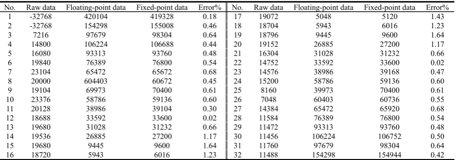
[image:7.595.74.541.528.692.2]

Image of solar granulation process (experimental data shown in Table 1), the results showed that data errors are about 1%. Such errors meet space solar telescope mirror placed in the related system requirements.

Table 1 Experimental data

No. Raw data Floating-point data Fixed-point data Error% No. Raw data Floating-point data Fixed-point data Error%

1 -32768 420104 419328 0.18 17 19072 5048 5120 1.43

2 -32768 154298 155008 0.46 18 18704 5943 6016 1.23

3 7216 97679 98304 0.64 19 18796 9445 9600 1.64

4 14800 106224 106688 0.44 20 19152 26885 27200 1.17

5 16080 93313 93760 0.48 21 16304 31028 31232 0.66

6 19840 76389 76800 0.54 22 14752 33592 33600 0.02

7 23104 65472 65672 0.68 23 14576 38986 39168 0.47

8 20000 604403 60672 0.45 24 15200 58786 59136 0.60

9 19104 69973 70400 0.61 25 8160 39973 70400 0.61

10 23376 58786 59136 0.60 26 7048 60403 60736 0.55

11 20128 38986 39104 0.30 27 14384 65472 65920 0.68

12 18688 33592 33600 0.02 28 11584 76389 76800 0.54

13 19680 31028 31232 0.66 29 11472 93313 93760 0.48

14 19536 26885 27200 1.17 30 11456 106224 106752 0.50

15 19680 9445 9600 1.64 31 11760 97679 98304 0.64

16 18720 5943 6016 1.23 32 11488 154298 154944 0.42

CONCLUSION

specific topology on solving parallel algorithm reduces the complexity and computational time complexity. Finally, the parallel fast Fourier transform algorithm combined with the practical, which resolves the contradiction between the rails large amounts of data in real time image processing and lack of aerospace grade DSP computing speed and improve the real-time processing capabilities. With the development of digital signal processing technology, the fast Fourier transform parallel algorithms in many practical problems will be widely used.

REFERENCES

[1]Yu Xiumin , Parallel Algorithms for Fast Fourier Transform, Chinese information technology,2005(10):203-205 [2] E.O. Brigham forward, Liu Qun translation 《Fast Fourier Transform》 Shanghai Science and Technology Press,1979(9):14-18

[3] Liu Zhaohui, Han Yueqiu, Implementation of FFT with FPGA Technology-Beijing Institute of Technology,

1999(02):58-61

[4] Geng Lihong,Sun Cai hong,Li Changsong.Chinese Journal of Electronics,2006(1):101-105

[5] Algorithms for Fast Fourier Transform Author:Ji Hu Xia Shengping Yu Wenxian Periodical Modern Electronic Technique,2001(08):88-93

[6] Sun Shixinet al. The Research of Parallel Algorithm Beijing: Mechanical Industry Press,2005(5):61-66. [7]Zhou Xinlun, Liu Jian, Liu ZhiHua. Digital Image Processing, Beijing: National Defense Industry Press,