Design Optimization of Plate Girder Using Generalized Reduced Gradient and Constrained Artificial Bee Colony Algorithms

International Journal of Emerging Technology and Advanced Engineering

304

Design Optimization of Plate Girder Using Generalized

Reduced Gradient and Constrained Artificial Bee Colony

Algorithms

F. Faluyi1 and C. Arum2

1

Research Scholar, Department of Civil Engineering, Federal University of Technology; Akure, Nigeria

2

Senior Lecturer, Department of Civil Engineering, Federal University of Technology; Akure, Nigeria

Abstract—The Generalized Reduced Gradient (GRG) algorithm available in Excel Solver, and the Constrained Artificial Bee Colony (CABC) algorithm were utilized to optimize the design of plate girder for minimum weight, given the span and grade of the material of the girder. The cross sectional areas of the girder and stiffeners were minimized subject to the provisions of the Code of Practice BS 5950: 2000, as well as the Steel Designers’ manual provisions. A typical example in the Steel Designers’ manual was used to test the design models (excel spreadsheet model for GRG and a Delphi program for CABC). The results obtained include curves of optimal pairs of web depth and web thickness, web depth and flange thickness, and flange width and flange thickness. A curve was also obtained which for a given web depth, gives the optimal cross sectional dimensions of the girder and the stiffener. Although the results obtained using the GRG and the ABC algorithms were very close, the GRG algorithm was slightly superior, giving a 7.44% reduction in area compared to the initial design.

Keywords— Constrained Artificial Bee Colony (CABC), Generalized Reduced Gradient (GRG), plate girder design.

I. INTRODUCTION

Optimization is a procedure through which the best possible values of decision variables are obtained under the given set of constraints and in accordance to a selected optimization objective function. The most common optimization procedure applies to a design that will minimize the total cost or maximize the possible reliability or any other specific objective. Fields of science and engineering, business decision-making and industry are all rich in problems that require the implementation of optimization approach.

In the face of increase in price of materials, civil engineers and manufacturers are forced to reduce the costs of construction and shorten the implementation period to maintain their competitiveness.

It is not just in civil engineering that the search for minimum weight is the main goal; quantity of material is an important factor in most design fields. Everyone naturally tries to achieve as much as possible using as little as possible. The ability of engineers to produce better designs relies on the techniques available for design optimization.

The main goal of this paper is to optimize the steel girder cross section in order to achieve minimum weight. The spacing of intermediate stiffeners will also be optimized.

II. OPTIMIZATION ALGORITHM

A. Generalized Reduced Gradient Method

International Journal of Emerging Technology and Advanced Engineering

305 If the economic model and constraints are linear this procedure is the Simplex Method of linear programming, and if no constraints are present it is gradient search.

The GRG method is based on the idea of elimination of variables using the equality Constraints. The idea of generalized reduced gradient is to convert the constrained problem into an unconstrained one by using direct substitution. The development of the generalized reduced gradient method follows that of constrained variation. The generalized reduced gradient method uses an approach which is to find an improved direction for the economic model and also to satisfy the constraint equations. Microsoft Excel Solver uses the Generalized Reduced Gradient (GRG2) algorithm for optimizing nonlinear problems. This algorithm was developed by Leon Lasdon, of the University of Texas at Austin, and Allan Waren, of Cleveland State University (Microsoft Inc. 2011).

B. Artificial Bee Colony Algorithm

Swarm intelligence has become a research interest to many research scientists of related fields in recent years. Bonabeau (1999) has defined the swarm intelligence as ―any attempt to design algorithms or distributed problem-solving devices inspired by the collective behaviour of social insect colonies and other animal societies‖ The classical example of a swarm is bees swarming around their hive. The Artificial Bee Colony (ABC) Algorithm for solving global optimization problems was developed in 2005 by Dervis Karaboga based on the idea of intelligent behaviour of honey bee swarm. Bee foraging behavior was studied and a new artificial bee colony (ABC) algorithm simulating this behaviour of real honey bees was developed for solving multidimensional and multimodal optimization problems.

In the ABC algorithm, the colony of artificial bees contains three groups of bees: employed bees, onlookers and scouts. The number of employed bees is equal to the number of food sources and an employed bee is assigned to one of the sources. In the ABC algorithm, while onlookers and employed bees carry out the exploitation process in the search space, the scouts control the exploration process. Every bee colony has scouts that are the colony’s explorers. The explorers do not have any guidance while looking for food.

They are primarily concerned with finding any kind of food source. The scouts are characterized by low search costs and a low average in food source quality (Karaboga and Bastuk, 2007). According to Karaboga (2007), in ABC algorithm, the position of a food source represents a possible solution to the optimization problem and the nectar amount of a food source corresponds to the quality (fitness) of the associated solution. An important difference between ABC and other swarm intelligence algorithms is that in the ABC, the solutions of the problem are represented by the food sources, not by the bees. The food source of which the nectar is abandoned by the bees is replaced with a new food source by the scouts which involves calculating a new solution at random. The employed bee of an abandoned food source becomes a scout. An onlooker bee chooses a food source depending on the probability value associated with that food source.

The basic steps of the algorithm as expressed by Karaboga (2005) are shown below:

 Send the scouts onto the initial food sources REPEAT

 Send the employed bees onto the food sources and determine their nectar amounts

 Calculate the probability value of the sources with which they are preferred by the onlooker bees.  Send the onlooker bees onto the food sources and

determine their nectar amounts

 Stop the exploitation process of the sources exhausted by the bees

 Send the scouts into the search area for discovering new food sources, randomly

 Memorize the best food source found so far UNTIL (requirements are met)

C. Constrained Artificial Bee Colony Algorithm

International Journal of Emerging Technology and Advanced Engineering

306 In order to adapt the ABC algorithm to solve constrained problems, Karaboga used Deb’s constrained handling method instead of the greedy selection process of the pure ABC algorithm.

Pseudo-code of the ABC algorithm according to Karaboga and Bastuk for Constrained Optimization problems is:

 Initialize the population of solution  Evaluate the population

 Cycle = 1  Repeat

 Produce new solutions for the employed bees by using

…..1

 Apply selection process based on Deb’s method  Calculate the probability values for the

solution using fitness of the solutions and the

constraint violation (CV) using

…… 2

Where CV is defined by

………….. 3

 Produce a new solution for each onlooker bee in the neighborhood of the solution selected

depending on and evaluate their fitness value  Apply selection process between and based

on Deb’s method

 Determined the abandoned solutions by using ―limit‖ parameter from the scout. If it exists, replace it with a new randomly produced solution by step 5

…… 4

 Memorize the best solution achieved so far  Cycle = cycle+1

 Until cycle = MCN(maximum cycle number)

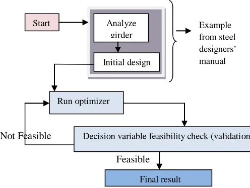
III. METHODOLOGY

The design optimization was carried out on an example in the Steel Designer’s Manual (2003) using Generalized Reduced Gradient (GRG2) nonlinear optimization algorithm found in Excel solver and Artificial Bee Colony (ABC) algorithm

The steps for is as highlighted below:

Carried out initial design (example from steel designer’s manual)

Optimization of the initial design using an optimizer Compared the final design result with the initial design to evaluate the success of the optimization (validation of result)

Not Feasible

Feasible

Figure 1: Optimization Process

A. Problem Formulation

This constrained optimization problem, which is a practical optimization problem, was formulated in terms of some parameters and restrictions. Mathematical formulation of the optimization problem in a standard mathematical function formula F(x) is described in the following sections. Stiffeners spacing was also maximized

Start Analyze girder

Initial design

Run optimizer

Decision variable feasibility check (validation)

Final result

International Journal of Emerging Technology and Advanced Engineering

307 d

T

t Wt

Wb

b

B. Design Parameters 1) Fixed Values

The fixed values arise from designed usage of the structure and code specifications, therefore could not be varied. In this case the fixed values are;

 Girder span  Steel yield strength

2) Design variables

The design variables in this structural optimization problem were the dimensions which control the cross– sectional area. These are the parameters that determine the geometry of the optimized girder.

They are;

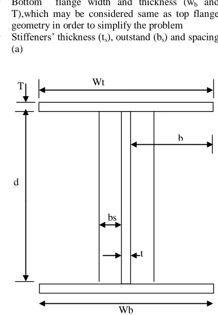
 Top flange width and thickness (wt and T)  Web height and thickness (d and t)

 Bottom flange width and thickness (wb and T),which may be considered same as top flange geometry in order to simplify the problem

 Stiffeners’ thickness (ts), outstand (bs) and spacing (a)

Figure 2: Welded Beam Section

920kN 92kN/m 920kN

3900 3900 56500mm

1550mm

30000mm

Figure 3: Beam Loading

C. Assumptions

Steel girder has a uniform cross section through its length

Web and flanges were made from the same homogenous material

The plate girder is simply supported

No longitudinal stiffeners are used; transfer stiffeners are used where necessary.

D. Design objective

The main objective is to minimize the weight given the design constraints. To minimize the weight, the cross section was minimized subject to the provisions in BS 5950-1(2000) and guides in Steel Designers’ Manual (2003).

The objective function;

Z = L{(wt x T) + (d x t) + (wb x T)} + {2(ts x bs x d)(L/a)}

Minimize Z subject to the following code/design constraints

E. Constraints

 Dimension/ sizing of plate girder element  Sectional classification/ proportional limitation  Moment resistance( flanges only method)  Shear capacity (strength)

 Serviceability  Stiffener Check 

International Journal of Emerging Technology and Advanced Engineering

308 Dimension/ Sizing of plate girder element

t ≥ d/250* minimum web thickness cl 4.4.3.2(BSI 2000)

t ≥ (d/250)(pyf/345)

where pyf is the compression flange strength.

The recommended span/depth ratio for simply supported non-composite girders varies between 12 for short span girders and 20 for long span girders.

L/20 ≤ d ≤ L/12 ………… (SCI,2003)

where L = length of girder

Section Classification / Proportional Limitation

Flange is assumed at least compact since the flange alone will resist the moment. Therefore;

b/T ≤ 9ε ……outstand element of compression flange (table 11. BSI 2000)

where ε = (275/ pyf) 0.5

pyf = 275 if T ≤ 16 265 if 16 <T ≤ 40

255 if 40 <T < 63

0.3d ≤ W ≤ 0.5d …………. (SCI,2003)

Note: W = 2b + t

W = width of flange

Moment resistance (flanges only method) (cl. 4.2.5 BSI 2000)

Mf > Mu

where Mu = maximum applied moment

Mf = pyf Af hs

hs = distance between centroid of flanges = d+T

Af = flange area

Shear capacity (without tension field action) (clause 4.4.5.1and 4, H.2 BSI 2000)

Since the web will likely be slender, i.e d/t > 62ε therefore shear buckling might be the governing criterion in the interior panels and critical shear buckling at the end panels.

Vcr> Fv

Vcr is the critical shear buckling resistance

If Vw = Pv, Vcr = Pv

If Pv >Vw > 0.72Pv, Vcr = (9Vw – 2Pv)/7

If Vw ≤ 0.72Pv, Vcr = (Vw/0.9)2/Pv

Fv is the maximum shear force;

Vw is the simple shear buckling resistance.

Vw = dtqw, Pv = 0.6pywdt Stiffner Check/Design

Maximum outstand of web stiffeners (clause 4.5.1.2 BSI 2000)

bs ≤ 13 ε ts

Spacing (clause 4.4.3 BSI 2000)

a > 1.5d

Minimum stiffness (clause 4.4.6.4 BSI 2000)

I > Is

Is = 0.75dt3min

I = ts x (2bs+t) 3

12

Load applied between stiffeners if the compression flange is restrained against rotation relative to the web (clause 4.5.3.2 BSI 2000)

Fed < Ped

where Fed = udl/t

and Ped = [2.75 + 2/ (a/d) 2] E/ (d/t) 2

F. Optimizers’ Settings

International Journal of Emerging Technology and Advanced Engineering

309

2) ABC Program: The parameters for the ABC algorithms were population (swam size), cycle, SPP (scout production period), perturbation rate and number of run.

Various settings were used but the best result was obtained with Population = 50, Cycle = 2000, SPP = 400, Perturbation rate = 1.0 and number of run = 50

IV. RESULTS AND DISCUSSION

A. Results

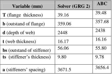
Though the solver settings were done with an intention of 200 iterations, it was however observed that after 10 iterations the solver stopped having reached convergence. For the ABC several runs were carried out with varying control settings. The reports are presented in Appendix 2. The best result is as shown in Table 4.1

TABLE I RESULT OF OPTIMIZED SECTION’S PARAMETERS

Variable (mm) Solver (GRG 2) ABC

T (flange thickness) 39.16 39.48

b (outstand of flange) 359.06 357.68

d (depth of web) 2448 2438

t (web thickness) 16.17 16.16

bs (outstand of stiffener) 56.06 55.80 ts (stiffener’s thickness) 9.80 9.78

a (stiffeners’ spacing) 3671.5 3656.4

The denotations are as earlier defined. It is important however to compare the initial design’s parameters with the result of the optimization. This is also presented in the table 4.2 below

TABLE II COMPARISON BETWEEN INITIAL AND OPTIMIZED SECTIONS’S

PARAMETERS

Optimized Section (mm)

Variable Initial Section (mm)

Solver (GRG

2) ABC

T 50 39.16 39.48

b 367.5 359.06 357.68

d 2000 2448 2438

t 15 16.17 16.16

bs 80 56.06 55.80

ts 15 9.80 9.78

a 3750 3671.5 3656.4

The optimization produced a 7.44% and 7.25% reduction in cross-sectional area for Solver and ABC respectively; if as assumed the elements are made from the same homogenous steel, this will translate into 7.44% and 7.25% reduction in weight as well. Since the outcome of the Solver (GRG 2) was better than ABC, the solver result was considered above that of the ABC. In real life design, while the flange width may not be subjected to space constraint, the depth of a girder is usually an issue in building. The headroom is of great importance in many designs both residential and industrial, therefore an optimization process was also carried out various depths. By keeping d constant while solver minimizes the other variables the response of the other variables (parameters) relative to the depth of the girder is shown in Table 4.4. Each trial converged after 10 iterations.

TABLE III PARAMETRIC OPTIMIZATION WITH VARIOUS WEB DEPTHS (d)

Variables (mm)

d= 2000

d= 2100

d= 2200

d= 2300

d= 2400

d= 2448

T 60 54.8 50 46 42.3 39.16

b 293.1 307.3 323 337 352 359.06

d(constant) 2000 2100 2200 2300 2400 2448

t 15.12 15.4 15.6 15.8 16 16.17

bs 44.85 47.35 49.86 52.36 54.86 56,06

ts 7.3 7.5 8 8 8 9.79

International Journal of Emerging Technology and Advanced Engineering

310

B. Discussion

From the closeness of the result obtained using Solver (Generalized Reduced Gradient Algorithm) and ABC (Artificial Bee Colony Algorithm) which is evolutionary, there is much assurance that the function was not trapped in the local minima thus lending credibility to the result.

As illustrated in Figure 4 it was observed that the reduction in depth (d) of the girder caused increase in thickness (T) of flange plate. This is logical since moment capacity is dependent on the flange area and depth of girder (for flange only method, moment resisting capacity is a product of flange area and the lever arm which is depth of girder). 35 40 45 50 55 60 65

1900 2000 2100 2200 2300 2400 2500 2600

web depth (d) mm

fl a n g e t h ic k n e s s ( T ) m m

Figure 4: Relationship between Web Depth and Flange Thickness

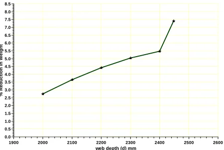
Figure 5 shows that increase in depth (d) of the girder translates to reduction in cross sectional area of the girder and by inference reduction in weight of girder. This shows that deeper girders are more economical. However, depth of girder cannot be increased infinitely due to headroom constraint and increasing susceptibility to web buckling.

0.96 0.97 0.98 0.99 1.00 1.01 1.02 1.03 ·105

1900 2000 2100 2200 2300 2400 2500 2600

Depth of web (d) mm

B e a m c ro s s -s e c ti o n a l a re a ( m m ) 2

Figure 5: Relationship between Web Depth and Cross- Section Area

0.0 0.5 1.0 1.5 2.0 2.5 3.0 3.5 4.0 4.5 5.0 5.5 6.0 6.5 7.0 7.5 8.0 8.5

1900 2000 2100 2200 2300 2400 2500 2600

web depth (d) mm

% R e d u c ti o n i n W e ig h t

International Journal of Emerging Technology and Advanced Engineering

311

15.0 15.5 16.0 16.5

1900 2000 2100 2200 2300 2400 2500 2600

Depth of web (d) mm

T

h

ic

k

n

e

s

s

o

f

w

e

b

(

t)

m

m

Figure 7: Relationship between Web Depth and Web Thickness

From Figure 7 abovethat there was slight increase in web thickness (t) with increase in depth of girder. This was probably influenced by the code provision to prevent occurrence of a web that is too slender.

560 580 600 620 640 660 680 700 720 740 760 780

36 38 40 42 44 46 48 50 52 54 56 58 60 62 64 Thickness of flange (T) mm

W

id

th

o

f

fl

a

n

g

e

(

W

)

m

m

Figure 8: Relationship between Flange Width and Flange Thickness

560 580 600 620 640 660 680 700 720 740 760 780

1900 2000 2100 2200 2300 2400 2500 2600

Depth of web (d) mm

W

id

th

o

f

fl

a

n

g

e

(

W

)

m

m

Figure 9: Relationship between Web Depth and Flange Width

From Figure 8 it was observed that the width of flange (W) reduces as the thickness of the flange (T) increases. Moment resistance depend on the product of these two variables (flange area), increase in one will only result in the decrease in the other.

V. CONCLUSION

This research has demonstrated how parametric optimization of a welded beam section can lead to significant reduction in weight of the beam. In particular, the GRG 2 algorithm yielded a 7.44% reduction in girder cross sectional area compared to the initial design while the ABC algorithm enabled a 7.25% reduction in the area.

References

[1] Adeli, H. & Sarma, K.C. 2006 Cost Optimization of Structures: Fuzzy Logic, Genetic Algorithms, and Parallel Computing. John Wiley & Sons, Ltd.

[2] Angira, R. & Babu, B. V. Evolutionary Computation for Global Optimization of

[3] Non-linear Chemical Engineering Processes,Department of Chemical Engineering; Birla Institute of Technology & Science, Pilani, India

[4] Anjos, M. & Zhang, H. 2006 Optimization and Engineering Applications, BIRS Workshop Report, Version 6

[5] Brajevic, I., Tuba, M. and Subotic, M 2011 Performance of The Improved Artificial Bee Colony Algorithm on Standard Engineering Constrained Problems; International Journal of Mathematics And Computer in Simulation, Issue 2, Volume 5, 2011 137

International Journal of Emerging Technology and Advanced Engineering

312

[7] Bonabeau, E., Dorigo, M. and Theraulaz, G. 1999 ―Swarm Intelligence: From Natural to Artificial Systems‖, Oxford University Press, New York.

[8] Deb, K 2000 An Efficient Constraint-handling Method for Genetic Algorithms, Computer Methods in Applied Mechanics and Engineering, Vol. 186, No. 0045-7825, 2000, pp. 311-338.

[9] Erwin 2009 Modeling with Excel+OML, a practical guide; Amsterdam Optimization Modeling Group LLC .

[10]Flager, F 2009 Interactive Collaborative Optimization – A Multidisciplinary Optimization Method Applied to the Design of Steel Building and Civil Structures. Center for Integrated Facility Engineering (CIFE), Stanford University, Stanford.

[11]Hinton, E. Sienz, J. Mustafa, O. 2003 Analysis and optimization of prismatic and axisymmetric shell structures. Springer

[12]Karaboga, D 2005 An Idea Based on Honey Bee Swarm For Numerical Optimization

[13]Technical Report -TR06, Computer Engineering Department, Erciyes University, Kayseri; Turkey

[14]Karaboga, D and Basturk, B 2007 Artificial bee colony(ABC) optimization algorithm for solving constrained optimization problems, Advances in Soft Computing: Foundations of Fuzzy Logic and Soft Computing, Vol. 4529/2007, No. 0302-9743, 2007, pp.789–798.

[15]Knight, R. P. 2003 Economical Steel Plate Girder Bridges, Journal of American Institute of Steel Construction.

[16]Lam, D. et al 2004 Structural Steelwork: Design to Limit State Theory 3e; Elsevier Butterworth-Heinemann,Linacre House, Jordan Hill, Oxford OX2 8DP 200 Wheeler Road, Burlington; MA 01803.

[17]Microsoft Support; (Accessed on 28 of October, 2011) Article Q82890, http://support.microsoft.com/kb/82890

[18]Rao, S.S. 2009 Engineering Optimization: Theory and Practice, Fourth Edition; John Wiley & Sons, Inc. New Jersey.

[19]Schreyer, A. C. 2005 Thermal and Structural Stud Wall Design Optimization in Excel Using Genetic Algorithms (Term Paper), Building Materials and Wood Technology Dept, University of Massachusetts, Amherst.

[20]Segui, G 1994 LRFD steel design, PWS Publishing Company.

[21]Steel Construction Institute (SCI) 2003 The Steel Designers’ Manual (6th _{Edition); Blackwell Publishing, London.}

[22]U.S. Department of Transportation, 2008 Final Report on Prefabricated Bridge Elements and Systems, United States Department of Transportation - Federal Highway Administration.

[22]Vasan, A. 2008 Optimization Using Differential Evolution, Department of Civil and Environmental Engineering; The University Of Western Ontario, London, Ontario, Canada.

[23]Vu, A.T. & Werner, F. 2009 Optimization of Steel Frame Structures Based on Differential Evolution Algorithm, 18th International

Conference on the Application of Computer Science and Mathematics in Architecture and Civil Engineering; Weimar, Germany.