Position Sensorless Control of a Permanent Magnet Stepping Motor Based on Sliding Mode Observer

(1)

Position Sensorless Control of a Permanent Magnet

Stepping Motor Based on Sliding Mode Observer

A. Mbarek, K. Ben Saad

*

_{, M. Benrejeb}

Research Unit LARA, National Engineering School of Tunis, ENIT BP 37, 1002 Tunis Belvédère *Corresponding Author: [email protected]

Abstract

This paper deals with a position sensorless

control of a permanent magnet stepping motor. The proposed controller is designed to reduce the studied actuator oscillations and overshoot which can induce an erratic working. As the mechanical solutions are expensive and cumbersome, the control ones are considered to be the most suitable. Closed loop control of these motors offers significant performance advantages. But, the use of position sensors complicates the drive design and its control system. To avoid the use of position sensors which are costly and cumbersome, we propose in this paper a sliding mode observer allowing the estimation of the motor position from the statoric voltages and currents. It is proven that a sliding mode observer is robust against observed systems parametric uncertainties and well adapted to a large variety of nonlinear systems such as electrical motors. The performances of the sensorless position proportional derivative controller and the robustness of the sliding mode observer are tested by numerical simulations. The obtained results show the efficiency of the proposed control law.

Keywords

Permanent Magnet Stepping Motor, Sliding

Mode Observer, Proportional Derivative Control, Robustness

1. Introduction

A stepping motor is an electromechanical actuator which produces incremental movements called steps. It is known by its positioning accuracy. Moreover, it is an actuator designed to operate in open-loop motion control [1, 2].

The stepping motor position evolution presents some oscillations and a long settling time which can disturb some applications requiring high positioning precision. Moreover, the oscillations can induce the motor, at some control frequencies, to an erratic working.

There are several solutions allowing the elimination of the stepping motor oscillations which can be classified into mechanical solutions and control solutions [1-7].

The mechanical solutions consist into connecting a mechanical reductor to the motor which is often costly or increasing friction at the expense of machine output.

The control solutions, more flexible than the mechanical ones, consist of closed-loop control solutions which require position sensor considered to be cumbersome and expensive [3]. Consequently, for the case of the stepping motors it is interesting to apply a position sensorless control.

In this paper, a position sensorless control based on a proportional derivative control is proposed to reduce the position oscillations of a stepping motor. The position of the studied actuator is estimated by a sliding mode observer.

This paper is organized as follows. In section 2, the studied stepping motor model is presented. The proposed Sliding Mode Observer is designed in section 3. In section 4, the proposed position sensorless stepping motor Proportional Derivative control is described.

2. Studied Stepping Motor Model

The studied bipolar permanent magnet stepping motor is described by the following differential nonlinear dynamical equations [1,4]:

( )

(

)

( )

sin( )

cos( )

sin cos

v f

di

L u Ri K p

dt di

L u Ri K p

dt

K f

d _i _p _i _p

dt J J

C sign J d

dt

α

α α φ

β

β β φ

φ

α β

θ

θ θ

θ

 ₌ ₋ ₊ _Ω 



 ₌ ₋ ₋ _Ω 



 Ω_{= −} ₋ ₋ _Ω 

 

− Ω

   _{= Ω}  

(1)

The application of the DQ transformation allows the transformation of the stationary coordinate system to the rotating one.

(2)

( )

cos( ) sin

sin cos

d q

u p p u

α β θ θ θ θ       =     ₋      

   

(2)

( )

cos( ) sin

sin cos

d q

i p p i

α β θ θ θ θ       =     ₋      

    (3)

The application of the DQ transformation yields to the following expressions:

( )

d

d d q

q

q q d

f q v

di

L _dt u Ri Lp i di

L u Ri Lp i K dt

C d

J K i f sign

dt J d dt φ φ θ

 ₌ ₋ ₊ _Ω

 

 ₌ ₋ ₋ _{Ω −} _Ω

 

Ω

 ₌ _{− Ω −} _Ω

   _{= Ω} 

(4)

The studied motor is characterized by the following electrical and mechanical parameters:

R 18= Ω _{; L 12 2mH}₌ _, _{; p 12}₌ _; _{J 6,67.10 kg m}₌ -7 _. 2 1

K 0 03V rad s, . .−

φ= ; Un =24V ; fv =0,21.0 N.s.rad-4 -1

5 f

C =10 N−

3. Proposed Sliding Mode Observer

Several methods of observer design have been proposed for different types of nonlinear models. Moreover, there are no systematic methods for designing a nonlinear observer. Sliding mode observers are known to be robust nonlinear observers [8-12]. In order to avoid the use of a position sensor a sliding mode observer allowing the estimation of the motor position and speed is proposed in the following.

3.1. Principle

With reference to the stepping motor model (1) and considering the stator currents as the system outputs, the dynamics of the proposed sliding mode observer can be constructed as follows [13]:

( )

(

)

( )

(

)

( )

(

)

( )

(

)

(

)

(

)

(

)

1 1 2 2 3 3

ˆ _ˆ _ˆ _ˆ ₁

sin ˆ ˆ ₁ ˆ ˆ ˆ _cos ˆ

ˆ _ˆ _ˆ _ˆ _ˆ

sin sin

ˆ ˆ

ˆ _ˆ _ˆ _ˆ



= − + Ω + 



 ₊ ₋

 

 = − − Ω + 

+ −

 Ω_{= −} ₋

− Ω − Ω

+ − + −

= Ω + − + −

f v

K

di _{R i} _p _u

dt L L L

K sign i i di _{R i} K

p u

dt L L L

K sign i i K

d _i _p _i _p

dt J C

f _sign

J J

K sign i i K sign i i d _{K sign i} _i _{K sign i} _i

dt φ α α α α α β φ β β β β φ α β

α α β β

θ θ θ θ θ             (5)

where

∧

denotes estimated value and K1, K2 and K3 are the observer gains which are determined by Lyapunov stability analysis.

Let the error difference between real state and the observer estimate defined as follows:

ˆ ˆ ˆ ˆ

i i i i i i

α α α

β β β

θ θ θ  = − 

= − 



Ω = Ω − Ω   = −      (6)

For a good estimation errors tend toward zeros.

From (5) and (6), the estimation errors dynamics of the sliding mode observer can be expressed as:

( )

(

)

( )

(

)

( )

(

( )

)

( )

(

)

( )

1 1 2 2 3 ˆ ˆ sin sin ˆ ˆ cos cos sin sin ˆ ˆ

ˆ sin ˆ sin

ˆ

= − + Ω − Ω −

= − − Ω − Ω −

Ω_{= −} ₋

− +

− Ω − − − Ω − Ω = Ω − −

 _          _ _ v f K

di _{R i} _p _p

dt L L

K sign i di _{R i} K

p p

dt L L

K sign i K

d _i _p _i _p

dt J

i p i p

f _{K sign i} _{K sign i} J

C

sign sign J

d _{K sign i} _K dt φ α α α β φ β β φ α β α β α β α θ θ θ θ θ θ θ θ

θ

_{( )}

3                        

 sign iβ

(7)

The sliding surface is defined as follows:

S S S i i α β α β   =     =    (8)

Consider the following positive definite Lyapunov function candidate [14, 15]:

(

)

2

1 2

V= iα+ + Ω +iβ  θ (9)

From equation (7) and equation (9) the time derivative of V can be expressed as:

( )

(

)

( )

(

)

( )

2 2 1 2 1 2 3 ˆ ˆ sin sin ˆ ˆ cos cos ˆ ˆ

ˆ sin ˆ cos

sin cos

ˆ

 

= − + _Ω − Ω _

 

− − + _−Ω + Ω _

 

− − Ω − _− + _

 

− _ − _

− Ω Ω − Ω

−Ω +

− Ω −

               v f K R

V i i p p

L L

K R

K i i i p p

L L

K f

K i i p i p

J J

K

i p i p

J C

signe signe J

K signe i signe i K signe i

φ

α α

φ

α β β

φ

β α β

φ α β α β α θ θ θ θ θ θ θ θ

θ θ

(

+signe i

( )

β

)

(3)

If the derivative of the chosen Lyapunov function is definite negative, the estimated state space variables converges asymptotically to the real ones [9,10].

Assume that: Ωsin

( )

pθ − Ωˆsin

( )

pθˆ < Ω2 max , we obtain:

( )

(

sin ˆsin ˆ

)

4max max

iα Ω pθ − Ω pθ < i Ω (11) where: iα = iβ <2i_max

We can also establish the following inequalities:

( )

(

( )

)

max max ˆ ˆ

sin cos sin

ˆ ˆ

ˆ _sin ˆ _cos ₈

i p i p i p

i p i p i

α β α

α β

θ θ θ

θ θ

Ω − + −

− + < Ω



(12)

( )

(

sign iα sign iβ

)

4 max

Ω  +  < Ω ₍₁₃₎

max max 4

θ θ

Ω <  Ω (14)

( )

(

sign iα sign iβ

)

4 max

θ  +  < θ ₍₁₅₎

By considering the inequalities (11), (12), (13), (14) and (15) we can deduce that:

2 2

max max 1 max

2

max max 2 max

max max 3 max

8 4

4 4

v

K

R R

V i i i K i

L L L

K

f _i _K

J J

K

φ

α β

φ

θ θ

< − − + Ω −

− Ω + Ω − Ω

+ Ω −

  

 ₍₁₆₎

As V must be negative definite to insure the convergence of the estimated space variables to the real ones, it is sufficient to choose the gains K1

,

K2

and

K3 so that:

1 max

2 max

3 max

2

K K

L K

K i

J K

φ

φ 

> Ω 

 

>  

> Ω   

(17)

3.2. Proposed Observer Validation

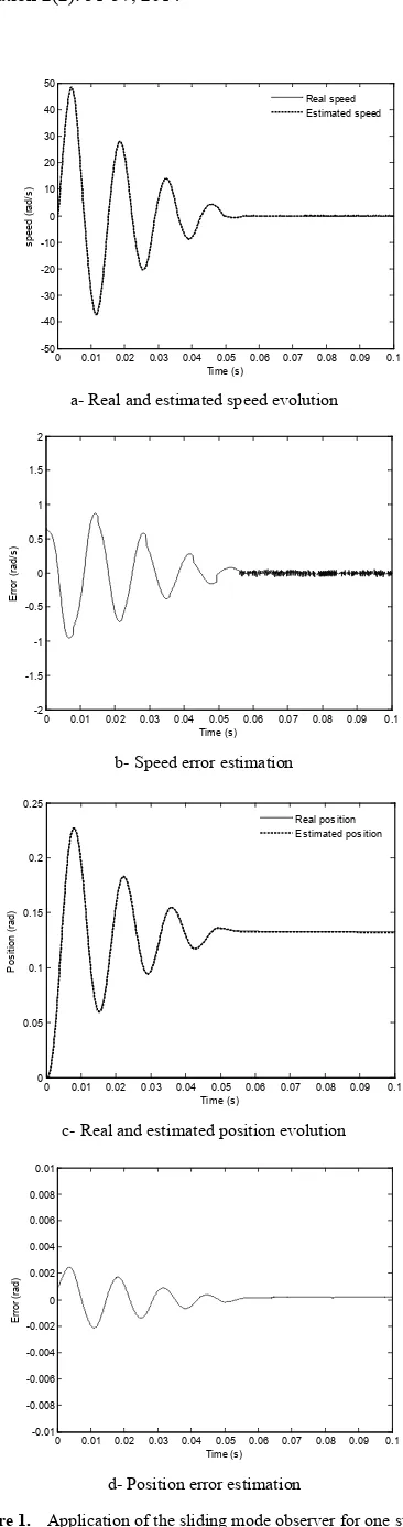
The proposed sliding mode observer is tested by numerical simulations. The first test is carried out by application of the nominal voltage to the motor. Thus the rotor moves with a step of 0.13 rad which is the studied motor elementary incremental movement. The obtained results are presented in Fig. 1. Fig.1-a and Fig. 1-b presents respectively the real and estimated rotor positions.

We can deduce that the observer allows the good estimation of the motor position and speed from the speed error estimation and the position error estimation Fig. 1-c and Fig.1-b.

a- Real and estimated speed evolution

b- Speed error estimation

c- Real and estimated position evolution

[image:3.595.339.522.43.736.2]

d- Position error estimation

Figure 1. Application of the sliding mode observer for one step

(

Uα=0 =, U Uβ n

)

0 0.01 0.02 0.03 0.04 0.05 0.06 0.07 0.08 0.09 0.1 -50

-40 -30 -20 -10 0 10 20 30 40 50

Time (s)

speed (

rad/

s)

Real speed Estimated speed

0 0.01 0.02 0.03 0.04 0.05 0.06 0.07 0.08 0.09 0.1 -2

-1.5 -1 -0.5 0 0.5 1 1.5 2

Time (s)

E

rro

r (ra

d/

s)

0 0.01 0.02 0.03 0.04 0.05 0.06 0.07 0.08 0.09 0.1 0

0.05 0.1 0.15 0.2 0.25

Time (s)

P

os

iti

on (

rad)

Real position Estimated position

0 0.01 0.02 0.03 0.04 0.05 0.06 0.07 0.08 0.09 0.1 -0.01

-0.008 -0.006 -0.004 -0.002 0 0.002 0.004 0.006 0.008 0.01

Time (s)

E

rro

r (ra

(4)

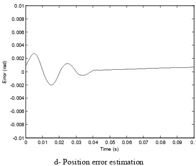
In order to generalize the obtained result, the observer was tested also for the case of one step position evolution and by application of the half of the nominal voltage. The obtained results are given in the Fig. 2.

[image:4.595.335.527.77.240.2]

Figure 2. Application of the sliding mode observer for one step

(

Uα=0 =, U U /β n 2

)

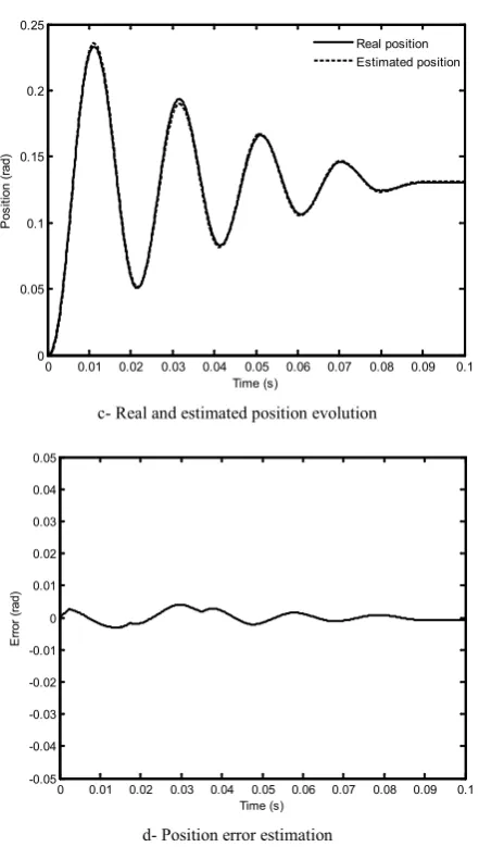
[image:4.595.67.534.131.696.2]

The robustness of the proposed was tested for the case of the rotor inertia variation. The obtained results, given by the Fig. 3, show the efficiency of the proposed nonlinear observer.

0 0.01 0.02 0.03 0.04 0.05 0.06 0.07 0.08 0.09 0.1 -50

-40 -30 -20 -10 0 10 20 30 40 50

Time (s)

S

peed (

rad/

s)

Real speed estimated speed

0 0.01 0.02 0.03 0.04 0.05 0.06 0.07 0.08 0.09 0.1 -2

-1.5 -1 -0.5 0 0.5 1 1.5 2

Time (s)

E

rro

r (ra

d/

s)

0 0.01 0.02 0.03 0.04 0.05 0.06 0.07 0.08 0.09 0.1 0

0.05 0.1 0.15 0.2 0.25

Time (s)

P

os

iti

on (

rad)

0 0.01 0.02 0.03 0.04 0.05 0.06 0.07 0.08 0.09 0.1 -0.01

-0.008 -0.006 -0.004 -0.002 0 0.002 0.004 0.006 0.008 0.01

Time (s)

E

rro

r (ra

d)

0 0.01 0.02 0.03 0.04 0.05 0.06 0.07 0.08 0.09 0.1 -50

-40 -30 -20 -10 0 10 20 30 40 50

Time(s)

S

peed (

rad/

s)

0 0.01 0.02 0.03 0.04 0.05 0.06 0.07 0.08 0.09 0.1 -5

-4 -3 -2 -1 0 1 2 3 4 5

Time (s)

E

rro

r (ra

d/

(5)

[image:5.595.68.289.70.460.2]

Figure 3. Application of the nonlinear observer for one step by increasing the rotor inertia (2×J)

4. Position Sensorless Stepping Motor

PD Control

4.1. Principle

In order to apply a PD control to eliminate the position oscillations, we propose to simplify the mathematical model of the studied stepping motor by considering a current control. For such case, the electrical equations are expressed as follows:

(

)

(

)

1 _{sin( )}

1 _{cos( )}

i u K p

R

i u K p

R

α α φ

β β φ

θ

 = + Ω

 

 = − Ω



(18)

Thus, by neglecting the dry friction, the mechanical equations describing the slow motor dynamic are given by the following expressions:

( )

(

)

2

sin cos

1 _v

K

u p u p

JR K f

J R

φ

α β

φ θ

θ θ

   = Ω 

Ω = − −

 

  

 −  + Ω

 

 _ _

 

 ₍₁₉₎

The application of the DQ transformation to the eq. (19) leads to the following linear equation:

2 1

q v

K K

u f

JR J R

φ φ

θ  = Ω

 _ _

 _ _

Ω = − − + Ω

 _ _

  





 (20)

From the eq. (20) we can define the following transfer function:

( )

₂

1 q

v

K u JR s

K

s s f

J R

φ

θ =

  

 +  + 

 

 _ _

 

(21)

The PD-controller transfer function is expressed as follows:

( )

p d

C s =K +K s₍₂₂₎ where:

p

K and K_d are respectively the proportional and integral gains,

ref

θ is the desired reference position.

The closed loop control system of model (21) can then be written as:

( )

(

₂

)

2 1

p d

v d p

K

K K s JR

s

K K K

s f K s K

J R JR JR

φ

φ φ φ

θ = +

        + _ + _+ +

 _ _ 

 

(23)

The determination of the Kp and Kd parameters can be done by a pole placement technique.

To avoid the use of a position sensor the PD control will be associated with the proposed sliding mode observer, fig. 4.

0 0.01 0.02 0.03 0.04 0.05 0.06 0.07 0.08 0.09 0.1 0

0.05 0.1 0.15 0.2 0.25

Time (s)

P

os

iti

on (

rad)

0 0.01 0.02 0.03 0.04 0.05 0.06 0.07 0.08 0.09 0.1 -0.05

-0.04 -0.03 -0.02 -0.01 0 0.01 0.02 0.03 0.04 0.05

Time (s)

E

rro

r (ra

(6)

[image:6.595.332.524.94.554.2]

Figure 4. Motor closed loop PD control strategy

4.2. Simulation Results

The simulation results obtained by application of the proposed sensorless position control are given by fig. 5. The figures 5-a, 5-b, 5-c and 5-d present the obtained position, speed and statoric currents of the phase α and β

respectively.

Fig. 5-a shows the real and the estimated position of the stepping motor where all the oscillations and the overshoot, observed for the one step open-loop position evolution, are eliminated.

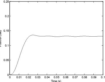
Fig. 6 gives the simulation results by increasing the rotor inertia two times. The obtained results prove the efficiency of the proposed control by association the proposed sliding mode observer.

a- Position evolution

b- Speed evolution

c- Phaseα current

[image:6.595.91.268.416.727.2]

d- Phase βcurrent

Figure 5. Application proposed sensorless controlled for one step

Figure 6. Position evolution (2×J) 0 0.01 0.02 0.03 0.04 0.05 0.06 0.07 0.08 0.09 0.1

0 0.05 0.1 0.15 0.2 0.25

Time (s)

P

os

iti

on (

rad)

0 0.01 0.02 0.03 0.04 0.05 0.06 0.07 0.08 0.09 0.1 0

5 10 15 20 25

Time (s)

S

peed (

rad/

s)

0 0.01 0.02 0.03 0.04 0.05 0.06 0.07 0.08 0.09 0.1 0

0.1 0.2 0.3 0.4 0.5 0.6 0.7 0.8

Time (s)

cu

rre

nt

(A

)

0 0.01 0.02 0.03 0.04 0.05 0.06 0.07 0.08 0.09 0.1 0

0.1 0.2 0.3 0.4 0.5 0.6 0.7 0.8

Time (s)

cu

rre

nt

(A

)

0 0.01 0.02 0.03 0.04 0.05 0.06 0.07 0.08 0.09 0.1 0

0.05 0.1 0.15 0.2 0.25

Time (s)

P

os

iti

on (

[image:6.595.343.523.583.724.2]

(7)

5. Conclusion

This paper presents a position senseless PD control for a permanent magnet stepping motor. The designed control is based on a sliding mode observer allowing the estimation of the motor position, speed and currents.

The proposed control approach has the advantage of not requiring a position sensor which is cumbersome and expensive. The simulation results prove the efficiency and the robustness of the sliding mode observer. Moreover, when the PD control is associated to the sliding mode observer it allows the elimination of the motor oscillations.

Nomenclature

iα, iβ : statoric currents

uα, uβ : statoric voltages

L : statoric inductance

R : statoric resistance Kφ : flux constant

p : number of pairs of poles

J : inertia v

f : viscous friction coefficient f

C _{: coefficient of dry friction} θ : rotor position

Ω : rotor speed n

U : nominal voltage d

i _{: direct axis current} q

i _{: quadratic axis current}

d

u : direct axis voltage q

u : quadratic axis voltage

REFERENCES

[1] P. Acarnley. Stepping motors: A guide to theory and practice, 4th edition, IEE Control Engineering series ¬63, London, 2002.

[2] K. Saad, A. Mbarek and M. Benrejeb. Determination of the switching times of the bang-bang control for a linear stepping

motor by Lyapunov functions, Studies in Informatics and Control (SIC), pp.393-406, Vol.17, No.4, December 2008. [3] T. R. Fredriksen. Applications of the closed-loop stepping

motor, IEEE Transaction on Automatic Control, Vol. AC-13, N° 5, pp.464-474, Oct.1968.

[4] A. Rachid. Régulateur électromécanique Techniques de

l’Ingénieur, Traité Génie Electrique, D7 540, pp. 1-22, 1996. [5] A. Mbarek, K. Ben Saad and M. Benrejeb. Position sensorless Fuzzy logic control based on a nonlinear observer for a permanent magnet stepping motor, International Review of Automatic Control (IREACO), Vol. 2, No. 5, September 2008.

[6] A. Mbarek, K. Ben Saad and M. Benrejeb. A position

sensorless control for a linear stepping motor, Sixth International Multiconference on Signals, Systems, and Devices, SSD 2009, Djerba.

[7] A. Mbarek, K. Ben Saad and M. Benrejeb. Position sensorless control of a permanent magnet stepping motor based on a nonlinear observer, International Conference on Communications, Computing and Control Applications, CCCA 2011, Hammamet.

[8] Z. Xu and M.F. Rahman. An improved stator flux estimation for a variable structure direct torque controlled IPM synchronous motor drive using a sliding observer, IAS 2005. [9] Z. Yhan and V. Utkin. Sliding mode observers for electric

machines–An Overview, IEEE 2002.

[10] J.J.E. Slotine, J.K. Hedrick, E.A. Misawa. A sliding mode observer for nonlinear system, J. Dynamic System Measurement and Control, pp. 421-434, 1987.

[11] C. Aurora and A. Ferrara, Speed regulator of induction motor: an adaptive sensorless sliding mode control scheme, Preceeding of the 2004 American Control Conference Boston, Massachusetts.

[12] S.M. Kim, W.Y. Han, S.J. Kim, Design of a new adaptive sliding mode observer for sensorless induction motor drive, Electric Power Systems Research 70, pp. 16-22,2004. [13] Y.J. Zhan, C.C. Chan and K.T. Chau, A novel sliding mode

observer for indirect position sensoring of switched reluctance motor drives, IEEE Transactions on Industrial Electronics, Vol. 46, No. 2, pp. 390-397, Avril 1999.

[14] F. Takeshi, S. Somboom and O. Shigeru, A position and

velocity sensorless control for brushless DC motors using an adaptive sliding mode observer, IEEE Transactions on Industrial Electronics, Vol. 39, No. 2, April 1992.